151
5
ANALYSYS OF TESTS FROM THE SGI CAMPAIGN
5.1 Introduction
Sodium cooled fast reactors represent, as mentioned in previous chapters, GEN IV systems chosen by the GIF in order to enhance the future contribution and benefits of nuclear energy utilization. The experience gained with this kind of reactors is considerable because of the several past power plants operating, as described in Chapter 2.
One of the most important safety concerns for these reactors is the assessment of the consequences of a Core Disruptive Accident, although the likelihood of its occurrence is very low. Therefore, the simulation of core disruptive accidents and the assessment of potential, thermal and mechanical energy in new reactor designs has attracted new interest, as a consequence of the renewed interest for SFR in the frame of Gen IV.
Also new simulation tools have been developed meanwhile that are now applied in this domain. In case of a severe accident, a mixture of molten fuel and steel vapour, which forms an expanding bubble, might be driven out of the damaged core into the sodium pool (the so-called expansion phase). This causes the sodium’s level raise and, consequently, the cover gas pressure’s increase (see
Fig.5.1).
Fig.5.1 - Scheme of CDA
Experiments dealing with the injection of a high pressure gas into a stagnant liquid pool, such as the demonstration fast breeder reactor program (FBDR) in Japan [1] or the previous campaigns performed by Tobin and Cagliostro [2], describe characteristic phenomena taking place during the expansion phase and are of interest for testing and benchmarking. In order to investigate further the mechanisms involved in this phase of the accident evolution, an experimental campaign called SGI (German acronym of “Schnelle Gas Injektion”) was performed in 1994 in former Forschungszentrum Karlsruhe, now KIT [3].
In addition to the experimental studies, the expansion phase’s knowledge needs numerical analyses focused on studying the effects of the bubble growth, of the interfacial instabilities and of the entrainment which plays a crucial role in the expansion phase [4-7]. Therefore, from the computational viewpoint, a simple and clear geometry together with the use of simple materials is helpful in the assessment of codes which need models to handle the complex phenomena involved in this phase.
5.2 Experimental facility
The SGI campaign was aimed to investigate the mechanisms and phenomena involved in the bubble expansion phase. In order to achieve this goal, an experimental facility, which reproduced in scale 1/30 the Clinch River Breeder Reactor (CRBR), was built by SRI International, California, and used in the Forschungszentrum Karlsruhe for a series of experiments. In these experiments, a certain amount of gas was injected into a water pool, aiming at reproducing the typical phenomenology of the expansion phase in a nuclear reactor, as shown in
Fig.5.2.
Fig.5.2 - SGI experiment
The facility consisted of two vessels connected through a short tube as it is shown in Fig.5.3. The first vessel was the so called ‘pressure vessel’, which was completely filled with nitrogen at 293.15 K and with a pressure ranging from 0.3 to 1.1 MPa. The second vessel was the so called ‘main vessel’ and it consisted of an acrylic cylinder with an inner diameter of 33 cm. Since it simulated the reactor coolant pool, it was partially filled with water and partially with air at 293.15 K at atmospheric pressure. Furthermore, inner walls were placed inside this vessel aimed at reproducing the reactor’s inner structures, such as the biological shield tank.
As said, the two vessels were connected through a short tube, which was closed by two sliding doors and a thin brass foil of 5 µm above the doors. The doors were opened by exploding hydrogen-oxygen gas which drove two pistons towards the doors, pushing them sideways in opposite directions. Their role was to open the gas flow cross section within a short time with the minimum disturbance of the gas flow. The metal foil was used in order to avoid movement of doors upon the water as shown from experiments carried out without it and it broke at the slightest pressure pulse at the beginning of the opening process.
Transient pressure values were recorded at five positions, that is at three different radii in the main vessel cover (P3, P4 and P5, see Fig.5.3) one in the pressure vessel (P1 see Fig.5.3) and one at the nozzle (P2, see again Fig.5.3). No pressure measurement was available in water in order to avoid disturbances in the growth of the bubble. The flow inside the upper vessel was recorded by using high speed cameras with about 7000 frames per second and the symmetry of the flow was monitored through five mirror pictures on two sides, one perpendicular to each other.
153 In order to track the movement of water, two horizontal rows of red marker beads, with a diameter of 4.8 mm and a density of 1026 kg/m3, were placed at different vertical positions. The density of beads was chosen to be as close as possible to water density, in order to neglect friction between water and beads.
Fig.5.3 - Scheme of the experimental facility for the SGI Campaign [4]
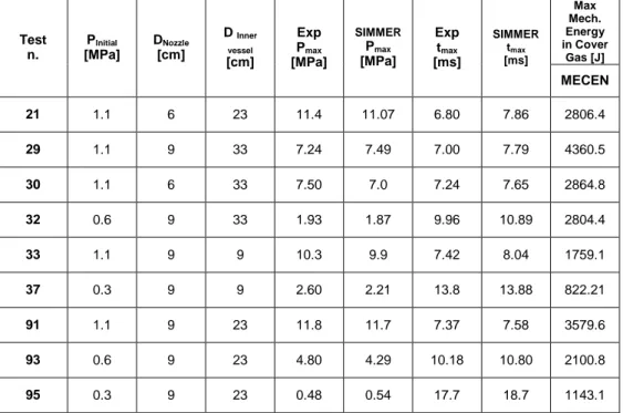
The campaign has investigated the effects of different injection pressures (0.3, 0.6 and 1.1 MPa) nozzle diameter (6 and 9 cm) and the presence of inner confinement walls on the formation of the rising bubble. Therefore, nine tests have been performed depending on these parameters, as shown in Table 5.1.
* inner vessel diameter means inner structure diameter (33 cm means no inner structure)
Table 5.1- Experimental Conditions of the nine performed tests [4]
In particular, tests 91, 93 and 95 were carried out with the same geometry, i.e. with the internal walls in the original configuration (see Fig.5.3), while for test n. 21 the bottom of the vessel was changed as in Fig.5.4, although the inner cylinder representing the biological shield tank was kept. This modification was aimed at simplifying geometry and bubble shape, even though it represented a departure from the original configuration.
A simplification of the geometry configuration, which was also an important parameter for the bubble expansion, was represented by the removal of the inner shield tank in the tests n. 29, 30, 32 (see Fig.5.5).
A completely different geometry was used in the tests n. 33 and n. 37, where a tall cylinder with the same diameter as that of the nozzle was added, aimed at preventing the radial expansion of the bubble (see Fig.5.6).
Fig.5.4 - Main vessel geometry for test n. 21
Fig.5.5 - Main vessel geometry for test for tests n. 29,30 and 32
155
Fig.5.6 - Main vessel geometry for test for tests n. 33 and 37
5.3 Geometrical model development and code qualification
Four tests, respectively 91, 93, 95, and 29, have been considered in the present work.
As mentioned, the first three tests have been performed with the same geometrical features that is the presence of an inner vessel wall with a diameter of 23 cm, height of 14 cm and the nozzle diameter equal to 9 cm. The only parameter changed has been the nitrogen injection pressure which has been respectively set equal to 1.1 MPa for test 91, 0.6 MPa for test 93 and 0.3 MPa for test 95 (see
Table 5.1).
Initial conditions for Test n. 29 differed from those of test n. 91 only for the absence of inner walls, thus allowing at assessing the influence of internal structures on the results (see again Table 5.1).
5.3.1 SIMMER III geometrical domain
All the tests chosen for the analysis have been simulated with SIMMER III. The simple cylindrical geometry is particularly suitable to be simulated in a 2D geometry, thus reducing uncertainties and allowing to qualify this version of the code.
Therefore, a cylindrical domain was set up for representing the test section used in tests n. 91, 93, 95 (see Fig.5.7). It is subdivided into 31 radial and 68 axial cells and, inside it, the main vessel is represented by the radial cells 1 - 31 and the axial cells 32 - 68. The cover gas region is included in the axial cells 56 - 68 and in the cells 1 - 31 radially, according to the volume data provided. The pressure vessel, the connection tube and the inner walls inside the main vessel are represented by ‘no calculation’ regions.
The experimental results concerning pressure, velocity and bubble growth have been compared with the simulations findings in order to qualify the code.
In addition, the results of these three tests have also been compared with the results obtained from simulation carried out with the FLUENT code [5]. Its flexible features make it suitable to deal with several different fluid dynamic problems concerning mixing, turbulence, chemical reactions thus allowing applications in several conventional industry fields [6] and including the nuclear industry [7]. This activity has been described in detail in [8].
The original domain was then modified in order to adapt it to the conditions of test n. 29 (compare Fig.5.7 and Fig.5.8).
Fig.5.7 - Test n. 91, 93 and 95 geometrical domain
Fig.5.8 - Test 29 geometrical domain
For this purpose, the ‘no calculation regions’ representing the inner structures have been removed and the water region was included in the cells 34 - 55, while radially the cells have remained unchanged (1 - 31).
5.3.2 Main results
The comparison among experimental main vessel pressure and SIMMER III and FLUENT results concerning test n. 91, 93 and 95 are shown in Fig.5.9, Fig.5.10 and Fig.5.11. For the sake of simplicity, only the maximum pressure among those detected from the three pressure gauges P3, P4, P5 (see Fig.5.3) in the cover gas region is shown, although all the pressures recorded in this region have been analysed, taking as reference cells corresponding to the positions of the pressure measurement devices.
Also for test n. 29, similarly to what has been done for the three previous tests, pressure results are shown just for the maximum pressure but in this case only the comparison between SIMMER III and experimental findings is available (see Fig 5.12).
157
Pinj 1.1 MPa Presence of Internal Structures
0.0 2.0 4.0 6.0 8.0 10.0 12.0
0.0E+00 3.0E-03 6.0E-03 9.0E-03 1.2E-02 1.5E-02 1.8E-02
Time [s] P re s s u re [ M P a ] Experimental SIMMER III FLUENT
Fig.5.9 - Test n. 91 main vessel maximum pressure
Pinj 0.6 MPa Presence of Internal Structures
0.0 0.5 1.0 1.5 2.0 2.5 3.0 3.5 4.0 4.5 5.0
0.0E+00 3.0E-03 6.0E-03 9.0E-03 1.2E-02 1.5E-02 1.8E-02
Time [s] P re s s u re [ M P a ] Experimental SIMMER III FLUENT
:
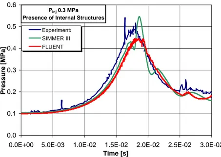
Pinj 0.3 MPa Presence of Internal Structures
0.0 0.1 0.2 0.3 0.4 0.5 0.6
0.0E+00 5.0E-03 1.0E-02 1.5E-02 2.0E-02 2.5E-02 3.0E-02
Time [s] P re s s u re [ M P a ] Experimental SIMMER III FLUENT
Fig.5.11 - Test n. 95 main vessel maximum pressure
Pinj 1.1 MPa
Absence of Internal Structures
0.0 1.0 2.0 3.0 4.0 5.0 6.0 7.0 8.0
0.0E+00 4.0E-03 8.0E-03 1.2E-02 1.6E-02 2.0E-02
Time [s] P re s s u re [ M P a ] Experimental SIMMER III
Fig 5.12 - Test n. 29 main vessel maximum pressure
As can be seen from Fig.5.9 to Fig.5.11, the higher is the injection pressure the higher is the maximum pressure value reached in the cover gas region. In fact, the gas bubble begins to grow inside water, raising the water level
159 and at the same time compressing the cover gas. The maximum pressure is reached at the moment when the bubble pushes the water up to the top of the main vessel and reaches its maximum dimension before it breaks up. As a consequence, the pressure decreases rapidly.
The comparison between experimental data and simulation results exhibits a good agreement for all the tests considered. In particular, for test n. 91 (see
Fig.5.9), the sharp peak of about 12 MPa at about 0.0074 s is well simulated both
regarding timing and pressure values reached. In the depressurization phase, SIMMER simulation, as well as FLUENT, show a second small peak. This second peak is less defined in the experiment than in the simulations and this might be probably due to a slight overestimation of the pressure wave from both codes. In fact, the presence of this wave, shown in both simulations, could be due to the reflection of the fluid from the wall, which is symmetric in SIMMER and FLUENT but not so perfectly symmetric in the experiment.
Experimentally, the pressure stabilizes at about 0.7 MPa after 0.009 s. SIMMER III results are in agreement with this trend, even though the calculated value is slightly lower than the experimental results (about 0.6 MPa). FLUENT results show some oscillations around a value of 0.7 MPa. It must be noted that after 0.015 s FLUENT evaluates a pressure increase up to 1.6 MPa, perhaps due to an overestimation of the initial bubble growth.
Concerning test n. 93 (see Fig.5.10), the experimental pressure trend looks similar to the test 91 trend, exhibiting a sharp peak of about 4.76 MPa at 0.01 s. Even the pressure decrease shows similarities with test n.91, although a series of three lower peaks can be noted during the phase of pressure decrease which lasts up to 0.016 s. Afterwards, the pressure stabilizes at about 0.35 MPa.
Even in this case, a good agreement between the two codes and the experiment is achieved, although some differences can be noted. The results of both codes are affected by a deviation from the experimental results, which starts for both at 0.0075 s. Consequently, comparing with the timing of reaching the experimental maximum value (10.8 ms, see Fig.5.10 and Table 5-2), SIMMER simulation presents a delay of 0.005 s and FLUENT 0.004 s. The peak value is underestimated, too. While SIMMER determines a peak of 4.3 MPa, FLUENT evaluates the maximum at 3.3 MPa. Furthermore, during the pressure decrease, the FLUENT curve shows three peaks that might be correlated to the three close peaks observed experimentally. Afterwards, both codes are in good agreement with experimental results.
Fig.5.11 shows the experimental and calculated pressure in the cover gas
region for Test n. 95, representing the lower extreme among the three tests chosen for this comparison, because of its lowest initial gas injection pressure (0.3 MPa). Due to the lower injection pressure, the bubble expands more slowly with respect to test 91, thus compressing the cover gas region in a weaker manner. Therefore, the experimental pressure peak reaches the maximum value of about 0.5 MPa in about 0.0175 s and the pressure variation shows a less rapid increase and decrease compared to the “spikes” observed in test n. 91 and test n.93 and a corresponding larger peak width.
Concerning the simulations, although test n. 95 confirms a quite good agreement between the codes and the experimental data, both codes show a small delay (about 0.001 s) in reaching the maximum. In particular, FLUENT underestimates slightly the pressure curve in its raising part, reaching a peak of about 0.45 MPa. The SIMMER pressure curve for the first 0.0165 s is located
between the experimental and the FLUENT curves. Afterwards, SIMMER evaluates a first peak which is sharper than in the experiment and then it overestimates the main spike, reaching a value of 0.546 MPa. Furthermore, the pressure decrease presents a steeper slope with respect of the other two curves and a lower peak at 0.022 s. From 0.025 s on, the results of both codes show some oscillations.
Removing the internal structures and injecting nitrogen at 1.1 MPa, as done in Test n. 29, the shape of the pressure variations shown in Fig 5.12 looks similar to that observed in Test n. 91. In fact, a sharp peak of 6.32 MPa arises at about 0.0071 s having also the same timing. From the simulation point of view, it must be noted an overestimation of the maximum (about 1.5 MPa higher in SIMMER simulation) and a slight shift of the overall curve. Despite this, SIMMER agrees well with experimental data, correctly reproducing also the oscillations following the depressurization phase.
It is worth noting that, in all the tests considered, the full width at half maximum of the simulations is in reasonable agreement for all curves shown in
Fig.5.9 through Fig 5.12.
The comparison of experimental and calculated pressure records in the pressure vessel is shown in Fig.5.13 through Fig.5.16. Generally, when the sliding doors open, nitrogen begins to flow into the water pool, causing the expanding bubble rise and, at the same time, decreasing the pressure in pressure vessel.
0.0 0.2 0.4 0.6 0.8 1.0 1.2 1.4
0.0E+00 3.0E-03 6.0E-03 9.0E-03 1.2E-02 1.5E-02 1.8E-02
Time [s] P re s s u re [ M P a ] Experimental SIMMER III FLUENT
161 0 0.1 0.2 0.3 0.4 0.5 0.6 0.7 0.8
0.0E+00 3.0E-03 6.0E-03 9.0E-03 1.2E-02 1.5E-02 1.8E-02
Time [s] P re s s u re [ M P a ] Experimental SIMMER III FLUENT
Fig.5.14 - Test n.93 lower vessel pressure
0.00 0.05 0.10 0.15 0.20 0.25 0.30 0.35 0.40
0.0E+00 5.0E-03 1.0E-02 1.5E-02 2.0E-02 2.5E-02 3.0E-02
Time [s] P re s s u re [ M P a ] Experimental SIMMER III FLUENT
0.0 0.2 0.4 0.6 0.8 1.0 1.2
0.0E+00 4.0E-03 8.0E-03 1.2E-02 1.6E-02 2.0E-02
Time [s] P re s s u re [ M P a ] Experimental SIMMER III
Fig.5.16 - Test n.29 lower vessel pressure
For Test n. 91 (see Fig.5.13) pressure reaches its minimum of 0.52 MPa at about 0.01 s and then the pressure starts to rise again. This is due to the break-up of the expanding bubble in the water region which decreases the pressure in the main vessel, allowing the lower vessel pressure to increase again. Both codes are in very good agreement with experimental data. SIMMER reproduces very closely experimental values and general trends, while FLUENT shows oscillations during the first 0.005 s and a small underestimation of the minimum pressure value and of the following pressurization phase.
The other two tests, n.93 and n.95 respectively, have highlighted similar pressurization trends (see Fig.5.14 and Fig.5.15) with a good agreement. Then, similarly to the simulation of test n.91, FLUENT tends to underestimate slightly the minimum pressure and the following pressurization phase while SIMMER reproduces more accurately the experimental trends.
In test n. 29, as shown in Fig.5.16, SIMMER reproduces almost perfectly the experimental transient up to 0.0087 s, while after that time, the simulation shows a slightly lower pressure minimum and a minor delay for its occurrence. During the re-pressurization phase the pressure increase in the experiment is somewhat more pronounced than that predicted by SIMMER.
The next parameter analysed has been the gas bubble growth. It must be pointed out that FLUENT allows to calculate directly the volume of the rising bubble, while this is not possible with the standard version of SIMMER. Thus a tool has been developed aiming at evaluating this important parameter. This tool has a “direct access read” to the base file SIMBF. The user can choose the region to be processed (in our case the water region) and the bubble volume is calculated as in the following. j i m n j i j i bubble
V
V
, , 1 , ,α
∑
==
(5.1)163 where α is the gas volume fraction, i, j are the indices of radial and axial cells, respectively and n,m represent the highest cells numbers of the monitored region in radial and axial direction. This simple algorithm is valid up to the bubble break up; then, it is no more possible to assess the bubble volume because of the mixing of cover gas and nitrogen bubble.
In any case also from the experimental point of view the data are available just for a very short time range that is the time range in which the rising bubble is well defined and measurable. The results obtained by the simulations and the experimental results are shown from Fig.5.17 to Fig.5.20.
Pinj 1.1 MPa Presence of Internal Structures
0.0E+00 5.0E-04 1.0E-03 1.5E-03 2.0E-03 2.5E-03 3.0E-03 3.5E-03 4.0E-03
2.0E-03 3.0E-03 4.0E-03 5.0E-03 6.0E-03
Time [s] V o lu me [ m 3 ] Experimental SIMMER III FLUENT
Pinj 0.6 MPa Presence of Internal Structures
0.0E+00 5.0E-04 1.0E-03 1.5E-03 2.0E-03 2.5E-03 3.0E-03
0.0E+00 2.0E-03 4.0E-03 6.0E-03 8.0E-03
Time [s] V o lu m e [ m 3 ] Experimental SIMMER III FLUENT
Fig.5.18 - Test n.93 bubble volume
Pinj 0.3 MPa
Presence of Internal Structures
0.0E+00 5.0E-04 1.0E-03 1.5E-03 2.0E-03 2.5E-03 3.0E-03 3.5E-03
0.0E+00 2.0E-03 4.0E-03 6.0E-03 8.0E-03 1.0E-02 1.2E-02
Time [s] V o lu m e [ m 3 ] Experimental FLUENT SIMMER III
165 Pinj 1.1 MPa
Absence of Internal Structures
0.0E+00 1.0E-03 2.0E-03 3.0E-03 4.0E-03 5.0E-03 6.0E-03 7.0E-03 8.0E-03 9.0E-03
0.0E+00 1.0E-03 2.0E-03 3.0E-03 4.0E-03 5.0E-03 6.0E-03 7.0E-03
Time [s] V o lu m e [ m 3 ] Experiment SIMMER III
Fig.5.20 - Test n.29 bubble volume
Test n.91 (see Fig.5.17) has highlighted a very good matching between SIMMER and FLUENT and, moreover, the almost identical results of both codes agree completely with the experimental data. For test n. 93 and n. 95, also very close agreement between the results of both codes has been found as is evident in
Fig.5.18 and Fig.5.19, although a slight deviation from the experimental data can
be noted with decreasing the injection pressure.
Concerning test n. 29, the absence of inner structures seems to cause a slight underestimation of the bubble volume by the simulation point of view (see
Fig.5.20 and compared with the excellent agreement between experimental and
calculation results shown in Fig.5.17), although the agreement with experiment is still rather good.
Summarizing, it is possible to conclude that the comparison between the experimental pressure curves and the numerical results obtained from SIMMER and FLUENT codes has established a good agreement, both for the main vessel and the pressure vessel.
Concerning the bubble volume assessment, the tool developed for calculating the bubble volume from SIMMER data provided matching values compared to FLUENT results, thus confirming the same small discrepancies with respect to experimental data. Therefore, this comparison has turned out to be important in order to qualify further results obtained by using the SIMMER III tool and to justify its use also in other simulations involving other materials, like LBE and water, as described in Chapter 4.
5.4 Energy evaluation
SGI experiments provided the possibility of having a critical look to BFCAL features. In fact, the experimental data highlighted that, inside the cover gas region, the expanding bubble creates three main zones with different pressures, such as a maximum, middle and a minimum pressure zone. Since BFCAL averages pressure values over the considered regions (see Chapter 4) and the regions cannot be divided radially, it is not possible to focus on special regions in order to assess possible local damages, such as, for example, the part of cover gas where the pressure reaches its maximum.
In addition, SGI experiments can be considered as ‘special cases’ for which BFCAL cannot be used unless materials involved in the experiments are declared in a different way. In fact, as explained in the previous chapter, this tool is able to distinguish fission gas, normally used in simulations as cover gas, and the other gases which contain traces of fuel or coolant which are not taken into account in the computation of cover gas pressure.
Instead in SGI tests simulated with SIMMER there is no difference, from a material point of view, between cover gas and injected nitrogen. Therefore, BFCAL is not able to distinguish between the different gases which are present in the region considered for calculation, that is for SGI nitrogen of the expanding bubble and the cover gas. Pressure of the expanding bubble is higher than that of the cover gas region, thus the pressure averaging carried out with BFCAL algorithm leads to an overestimation of the pressure value of the region considered.
The closed system approach of BFCAL is, under these conditions not valid anymore.
These considerations have suggested to develop another post-processing tool for the SIMMER III basefile (SIMBF). The post processing tool, which is called MECEN and which is written in FORTRAN, is aimed at assessing kinetic energy, compression work and, therefore, the mechanical energy due to a expansion of the bubble which is representative of CDA.
The program may consider the overall domain, even though the calculation may be performed for a certain region of the domain that is chosen by the user. In this way, it is possible to perform analyses of particularly interesting regions. The aim of MECEN program can be better understood just by considering the SGI campaign.
As mentioned before, the three pressure gauges P3, P4 and P5 (see
Fig.5.3) detect three different values at three different radii in the pressure
continuum of the cover gas region. BFCAL, as mentioned in Chapter 4, does not give the possibility to divide the region considered for analysis (for the SGI cover gas region) into several radial regions and the pressure is averaged over just one radial region.
Referring, for instance, to test n.91 pressure values range from 11.8 MPa to 3.35 MPa and the averaging gives a pressure of about 7.6 MPa. This may be representative for assessing the membrane stress but it is clear that the evaluation of the effects due to higher local pressure, such as 11.8 MPa in test n.91, cannot be taken into account, even though they might play a role in local vessel deformations. MECEN gives the possibility to the user to focus on a particular local region (i.e. for SGI n. 91 the region of the maximum pressure) in order to assess energy release in that specific region, thus getting useful information for evaluating local stresses.
167 Obviously, mechanical energy is assessed through the sum of kinetic energy, compression work and energy due to gravitational forces. The work due to the gravitational forces gives a small contribution compared to the other two, so it can be considered negligible. However, the coolant velocities resulting from the conservation equations, which take into account the gravitational force, are read directly from the code. Therefore, this contribution is taken into account implicitly.
The kinetic energy of the coolant pool movement is turned into work and the process will eventually be terminated because of energy losses by internal dissipation and fluid-structure interaction. Considering our calculation domain, it can be defined as
)
(
2
1
2 , 1 1 2 , , i j n i m j j i j i L kinV
v
u
E
∑∑
= =+
=
ρ
(5.2)where ρL is the average liquid coolant mass for the cell volume, Vi,j is the cell volume, v and u are the axial and radial velocity of the coolant at the cell centre, respectively and i and j the indices for radial and axial cells. The work performed on the cover gas is strongly affected by the conversion of kinetic energy into compression work, when the coolant pool is decelerated.
Considering each time step k, compression work can be evaluated as
)
)(
(
2
1
1 ), , ( , , 1 ), , ( 0 , , 1 1 , − − = = =−
+
=
∑∑∑
i j k i jk i j k t k k j i n i m j j i workccV
p
p
E
α
α
(5.3)where Nt is the time step, p is the pressure of every cell and αis the gas volume fraction. The RHS term must be calculated all over the cover gas cells.
As previously mentioned, for these simulations the closed system approach is not anymore suitable. For this purpose, a check aimed at excluding cells which contain the entering nitrogen has been set up. In particular, starting from the lower cells of the region considered, cells are scanned in order to verify if their gas contents exceed a certain limit. If the gas volume fraction is beyond that limit the corresponding cells are excluded from the calculation.
Once kinetic energy and compression work are evaluated, it is possible to determine mechanical energy by
workcc kin
mech
E
E
E
=
+
(5.4)5.4.1 Analysis of the tests considered
Once the tool MECEN has been set up, the energy assessment of the four tests considered in the preliminary activity was carried out. The energy evaluation for Test n.91, 93, 95 and 29 in the cover gas region is shown in Fig.5.21 trough
Pinj 1.1 MPa Presence of Internal Structures
0.0E+00 5.0E+02 1.0E+03 1.5E+03 2.0E+03 2.5E+03 3.0E+03 3.5E+03 4.0E+03
0.0E+00 5.0E-03 1.0E-02 1.5E-02 2.0E-02 2.5E-02 3.0E-02
Time [s] E n e rg y [ J ] Kinetic Energy Compression Work Mechanical Energy
Fig.5.21 - Kinetic energy, compression work and mechanical energy in Test n. 91
Pinj 0.6 MPa Presence of Internal Structures
0.0E+00 5.0E+02 1.0E+03 1.5E+03 2.0E+03 2.5E+03 3.0E+03
0.0E+00 5.0E-03 1.0E-02 1.5E-02 2.0E-02 2.5E-02 3.0E-02
Time [s] E n e rg y [ J ] Kinetic Energy Compression Work Mechanical Energy
Fig.5.22 - Kinetic energy, compression work and mechanical energy in Test n. 93
169
Pinj 0.3 MPa Presence of Internal Structures
0.0E+00 2.0E+02 4.0E+02 6.0E+02 8.0E+02 1.0E+03 1.2E+03 1.4E+03
0.0E+00 5.0E-03 1.0E-02 1.5E-02 2.0E-02 2.5E-02 3.0E-02
Time [s] E n e rg y [ J ] Kinetic Energy Compression Work Mechanical Energy
Fig.5.23 - Kinetic energy, compression work and mechanical energy in Test n. 95
Pinj 1.1 MPa Absence of Internal Structures
0.0E+00 1.0E+03 2.0E+03 3.0E+03 4.0E+03 5.0E+03 6.0E+03
0.0E+00 5.0E-03 1.0E-02 1.5E-02 2.0E-02 2.5E-02 3.0E-02
Time [s] E n e rg y [ J ] Kinetic Energy Compression Work Mechanical Energy
Fig.5.24 - Kinetic energy, compression work and mechanical energy in Test n. 29
As can be seen in all the figures, the kinetic energy trend is characterized by a first maximum peak, which is due to the injection of gas that pushes up the water around the bubble. Then, a rapid decrease of the energy is caused by the bubble breakup. In this moment, the main vessel is filled with a mixture of water, nitrogen and cover gas that forms vortixes inside the vessel. The subsequent second peak is due to the water entering the pressure vessel, which causes the ejection of a certain amount of nitrogen at the same time. Once the second peak is reached, the kinetic energy tends asymptotically to zero because of the fluid-structure interaction and dissipation phenomena involved.
Also compression work (see Fig.5.21 - Fig.5.24) has exhibited the same tendency for all the tests considered. In fact, all the trends are characterized by the presence of a maximum peak, which is reached when the minimum of kinetic energy is achieved. This is affected by the conversion of the kinetic energy into compression work when the water pool is decelerated. Obviously mechanical energy, being given by the sum of the kinetic energy and compression work, reflects kinetic energy and compression work trends.
It is worth noting that the gas injection pressure plays an important role in the assessment of kinetic energy and compression work. In fact, kinetic energy tends to have maximum values closer to maximum conversion work values if the injection pressure is higher. Otherwise, as can be observed in Fig.5.23, which corresponds to an injection pressure of only 0.3 MPa, the difference between the two maxima is substantial. As could be expected, the relative contribution of kinetic energy becomes smaller with decreasing injection pressure.
The results from test n. 29 (see Fig.5.24 in comparison with Fig.5.21) show that for high injection pressure the amplitudes of kinetic energy and compression work are almost equal (~ 3·103 Joule), similarly to what has been observed for test n.91 where the kinetic energy differs from compression work just for about 2·102 Joule and both are in the order of about 2·103 Joule.
However, the absence of inner structures enhances the growth of the bubble which is free to expand radially in the water region. Therefore nitrogen injection is faster than in test n.91 as well as, at the same time, the bubble volume growth rate increase (compare also Fig.5.20 with Fig.5.17).
In addition as can be seen in Fig.5.25 through Fig.5.30, where the vectors of the bubble gas velocity (Q3 in the figures, starting from a base velocity of 200 m/s) the absence of inner structures intensifies the formation of vortexes compare to the case of presence of inner structures, thus enhancing the entrainment. As a consequence, the gas injection velocity is strongly increased and the amplitude of the kinetic energy and compression work turns out to be higher than in test n.91.
171
Fig.5.25 - Bubble velocity path in Test n. 91 (t =0.003 s)
Fig.5.26 - Bubble velocity path in Test n. 29 (t =0.003 s)
Fig.5.27 - Bubble velocity path in Test n. 91 (t =0.006 s)
Fig.5.28 - Bubble velocity path in Test n. 29 (t =0.006 s)
173
Fig.5.29 - Bubble velocity path in Test n. 91 (t =0.008 s)
Fig.5.30 - Bubble velocity path in Test n. 29 (t =0.008 s)
Moreover, the conversion of kinetic energy into compression work is strongly enhanced because the dissipative phenomena induced by the presence of
inner structures are strongly reduced. The wavy trend observed for the compression work after the first peak is probably due to the greater freedom of the gas to move inside the systems and mixing together with the other gas and water.
The comparison between the four tests concerning kinetic energy, compression work and mechanical energy, shown in Fig.5.31 - Fig.5.33, allows to illustrate the influence of various parameters.
0.0E+00 5.0E+02 1.0E+03 1.5E+03 2.0E+03 2.5E+03 3.0E+03 3.5E+03 4.0E+03
0.0E+00 5.0E-03 1.0E-02 1.5E-02 2.0E-02 2.5E-02 3.0E-02 Time [s] E n e rg y [ J ]
SGI 29 - no inner structures - Pinj 1.1 MPa SGI 91 - inner structures - Pinj 1.1 MPa SGI 93 - inner structures - Pinj 0.6 MPa SGI 95 - inner structures - Pinj 0.3 MPa
Fig.5.31 - Kinetic energy evaluation in the four tests considered
0.0E+00 5.0E+02 1.0E+03 1.5E+03 2.0E+03 2.5E+03 3.0E+03 3.5E+03 4.0E+03
0.0E+00 5.0E-03 1.0E-02 1.5E-02 2.0E-02 2.5E-02 3.0E-02 Time [s] E n e rg y [ J ]
SGI 29 - no inner structure - Pinj 1.1 MPa SGI 91 - inner structure - Pinj 0.6 MPa SGI 93 - inner structure - Pinj 0.6 MPa SGI 95 - inner structure - Pinj 0.3 MPa
Fig.5.32 - Compression work evaluation in the four tests considered
Regarding kinetic energy (see Fig.5.31), it is possible to note that test n.29 and test n.91, which have been carried out with the same injection pressure of 1.1 MPa, show the same shape, even though the values reached and the width of the
175 first peak are larger in case of absence of inner structure. In addition, the increase of the kinetic energy in test n. 91 is substantially delayed with respect to test n.29. Comparing test n. 91 with tests n.93 and n.95 (see Fig.5.31) it is clear that the softening of the first energy peak is strongly affected by the gas injection pressure. In fact, the two peaks highlighted in Test n. 91 become lower and wider as the injection pressure decrease, showing also an increasing delay.
Also from the point of view of compression work, the three tests previously mentioned show a delay associated to the injection pressure decrease (see
Fig.5.32). Similarly to what observed for the kinetic energy, even for compression
work tests n. 91, n. 93 and n. 95 highlight a broadening of the peak and a delay in reaching the maximum correlated with the injection pressure decrease. Instead, test n. 91 and test n.29, exhibit almost the same timing in reaching the maximum peak values, even though the pressure peak is lower in case of presence of inner structures. This represents a further confirmation of the importance of the initial pressure conditions.
Analysing mechanical energy trends of the four tests (see Fig.5.33) it is evident that, as expected, the maximum values decrease with decreasing the injection pressure. 0.0E+00 1.0E+03 2.0E+03 3.0E+03 4.0E+03 5.0E+03 6.0E+03
0.0E+00 5.0E-03 1.0E-02 1.5E-02 2.0E-02 2.5E-02 3.0E-02
Time [s] E n e rg y [ J ]
SGI 29 - no inner structure - Pinj 1.1 MPa SGI 91 - inner structure - Pinj 1.1 MPa SGI 93 - inner structure - Pinj 0.6 MPa SGI 95 - inner structure - Pinj 0.3 MPa
Fig.5.33 - Mechanical energy evaluation in the four tests considered
In addition, because the lower is the injection pressure the lower is the kinetic energy, the double peak due to kinetic energy contribution tends to be mitigated as the pressure decreases, up to the “extreme case” represented by test n. 95 where, considering a time range longer than that shown in Fig.5.33, can be claimed that a single low and broad peak is present and then mechanical energy tends to smooth.
Considering tests n. 91 and n. 29 it is possible to see that the presence of internal structure may mitigate the mechanical energy release. Results concerning some experimental parameters of the tests carried out in the whole SGI campaign are summarized in Table 5.1. The energy determined in all tests has been
evaluated by MECEN for the sake of simplicity just the maximum values of mechanical energy are reported. From this table is possible to note the good agreement between experimental parameters and simulation results.
In addition, from results obtained with MECEN, it is possible to deduce that from the energy point of view the absence of inner structures plays a crucial role. In fact, test n. 29 has shown the highest maximum mechanical energy value among the tests performed, despite the fact that the maximum pressure in the cover gas region was achieved in Test n.91.
Max Mech. Energy in Cover Gas [J] Test n. PInitial [MPa] DNozzle [cm] D Inner vessel [cm] Exp Pmax [MPa] SIMMER Pmax [MPa] Exp tmax [ms] SIMMER tmax [ms] MECEN 21 1.1 6 23 11.4 11.07 6.80 7.86 2806.4 29 1.1 9 33 7.24 7.49 7.00 7.79 4360.5 30 1.1 6 33 7.50 7.0 7.24 7.65 2864.8 32 0.6 9 33 1.93 1.87 9.96 10.89 2804.4 33 1.1 9 9 10.3 9.9 7.42 8.04 1759.1 37 0.3 9 9 2.60 2.21 13.8 13.88 822.21 91 1.1 9 23 11.8 11.7 7.37 7.58 3579.6 93 0.6 9 23 4.80 4.29 10.18 10.80 2100.8 95 0.3 9 23 0.48 0.54 17.7 18.7 1143.1
Table 5-2. Experimental and SIMMER results concerning all the tests carried out in the whole SGI campaign
5.5 Concluding remarks
The SGI experimental campaign was aimed at investigating the phenomena involved in the expansion phase following a CDA. The experimental facility was characterized by a cylindrical geometry that, together with the availability of several parameters, allowed a correct simulation of the overall campaign at best with the 2D version of the SIMMER code.
The simulation activity was carried out with the SIMMER III code for the whole test series. As a complementary activity, three tests, respectively n. 91, n. 93 and n. 95, were simulated also with FLUENT. Pressure in the main vessel and in the pressure vessel and bubble volume have been chosen as the main parameters to be compared with experimental data. In general, SIMMER III has highlighted a good agreement with the experimental results for all the tests of the experimental campaign. In particular, for the three tests considered for the comparison with FLUENT code, SIMMER III has shown comparable capabilities with respect to the CFD code in reproducing the experimental data, allowing to get similar results and saving, at the same time, computational resources and time.
177 The assessment of the bubble volume was carried out for SIMMER III by developing and implementing a specific tool, while in FLUENT this parameter can be directly extracted from the results of the simulations. The matching of the results of the two codes and their good agreement with experimental data allowed to qualify the SIMMER related tool, thus allowing to use it also for other kind of simulations.
This preliminary activity of code qualification was aimed at providing a basis for the energy assessment. In fact, if the simulation of the experiments confirmed good agreement with relevant experimental data, it is possible to suppose that also the energy assessment will be accurate.
Energy assessment has revealed limits in the applicability of the BFCAL tool, thus initiating the development of a new post processing tool for SIMMER III called MECEN.
The analysis of the kinetic energy, compression work and correlated mechanical energy has evidenced that the gas injection pressure plays a crucial role in energy behavior. In fact, the higher is the injection pressure the higher is the energy released in the test.
In addition, as the injection pressure decreases, the delay in reaching the maximum energy increases. This can be observed also from the pressure trends and bubble volume growth. A further comparison between test n. 91 and test n. 29 (see Fig.5.33) has shown the role of the internals in the mechanical energy release, whose presence decreases the amount of kinetic energy, compression work and therefore mechanical energy released in the test.
REFERENCES
1. Nakamura T., Kaguchi H., Ikarimoto I., Kamishima Y., Koyama K., Kubo S., Kotake S., “Evaluation method for structural integrity assessment in core disruptive accident of fast reactor”, Nucl. Eng. Des., Vol. 227, pp. 97 - 123, 2004.
2. Tobin R.J., Cagliostro D.J., “Energetics of simulated HCDA bubble expansions: some potential attenuation mechanisms”, Nucl. Eng Des., Vol. 58, pp. 85 - 95, 1980.
3. Meyer L., Wilhelm D., “Investigation of the Fluid Dynamics of a Gas jet Expansion in a liquid Pool”, Technical Report KfK5307, Forschungszentrum Karlsruhe, 1994.
4. Morita K., Matsumoto T., Fukuda K., “Experimental Verification of Fast Reactor Safety Analysis Code SIMMER III for Transient Bubble Behaviour with Condensation”, Proceedings of Technical Meeting on Severe accident and Accident Management Toranomon Pastoral, Minato-ku, Tokio, Japan , March 14th-16th, 2006.
5. Fluent Inc., “FLUENT 6.3 User's Guide”, February 2003.
6. Rider W.J., Kothe D. B., “Reconstructing Volume Tracking”, Journal of Computational Physics, Vol. 141, Issue 2, April 1998.
7. Di Marco P., Forgione N., Tarantino M. , “Analysis of the transient rise of an initially spherical gas bubble in a stagnant liquid”, Proceedings XXIV National Congress UIT on Heat Transfer, Napoli, Italy, June 2006.
8. Pellini D., Maschek W., Forgione N., Poli F., Oriolo F., “Simulation of Fast Gas Injection Expansion Phase Experiments” , Proceedings of the 18th International Conference on Nuclear Engineering, ICONE18, Xi’an, China, Paper n.29453, May 17th – 21th, 2010.