12- VORTEX TUBE

(1)

Experimental Study

on

the Ranque-Hilsch Vortex Tube

PROEFSCHRIFT

ter verkrijging van de graad van doctor aan de Technische Universiteit Eindhoven, op gezag van de Rector Magnificus, prof.dr.ir. C.J. van Duijn, voor een commissie aangewezen door het College voor Promoties in het openbaar te verdedigen op

dinsdag 29 november 2005 om 16.00 uur

door

Chengming Gao

geboren te HuBei, China

(2)

Dit proefschrift is goedgekeurd door de promotor: prof.dr. A.T.A.M. de Waele

Copromotor:

dr.ir. J.C.H. Zeegers

Copyright c_{°2005 C. Gao} Omslagontwerp: Paul Verspaget, Druk: Universiteitsdrukkerij, TUE

CIP-DATA LIBRARY TECHNISCHE UNIVERSITEIT EINDHOVEN Gao, Chengming

Experimental study on the RanqueHilsch vortex tube / door Chengming Gao. -Eindhoven : Technische Universiteit -Eindhoven, 2005.

Proefschrift. - ISBN 90-386-2361-5 NUR 924

Trefw.: Fysische transportverschijnselen / Gassen: Thermodynamica / Kolkstroming/ Tur-bulentie / Cryogene techniek.

Subject headings: Transport processes / Thermodynamics / Swirling flow / Turbulence / Cryogenics.

(3)

———To

My mother: Gao Cuihua; my father: Lee Kejing; My sister: Lee Yinxia

(4)

“In the experimental research, the appropriate experimental technology may achieve twice the result with half the effort.”

(5)

Chapter 1 Introduction

1.1 Background

The Vortex Tube (VT) cooler is a device that generates cold and hot gas from compressed gas, as shown in Fig. 1.1. It contains the following parts: one or more inlet nozzles, a vortex chamber, a cold-end orifice, a hot-end control valve and a tube. When high-pressure gas (6 bar) is tangentially injected into the vortex chamber via the inlet nozzles, a swirling flow is created inside the vortex chamber. When the gas swirls to the center of the chamber, it is expanded and cooled. In the vortex chamber, part of the gas swirls to the hot end, and another part exists via the cold exhaust directly. Part of the gas in the vortex tube reverses for axial component of the velocity and move from the hot end to the cold end. At the hot exhaust, the gas escapes with a higher temperature, while at the cold exhaust, the gas has a lower temperature compared to the inlet temperature. This was first discovered by Ranque [1] in 1933, and by Hilsch [2] in 1947. In memory of their contribution the VT is also known as Ranque Vortex Tube (RVT), Hilsch Vortex Tube (HVT), and Ranque-Hilsch Vortex Tube (RHVT). In this thesis it is referred to as Ranque-Hilsch Vortex Tube (RHVT).

A RHVT has the following advantages compared to the normal commercial refrigeration device: simple, no moving parts, no electricity or chemicals, small and lightweight, low cost, maintenance free, instant cold air, durable (because of the stainless steel and clean working media), adjustable temperature [3, 4]. But, its low thermal efficiency is a main limiting factor for its application. Also the noise and availability of compressed gas may limit its application. Therefore, when compactness, reliability and lower equipment cost are the main factors and the operating efficiency becomes less important, the RHVT becomes a nice device for heating gas, cooling gas, cleaning gas, drying gas, and separating gas mixtures, DNA application, liquefying natural gas and other purposes [3, 5–7].

The underlying physical mechanism processes that determine the cooling of gas in this device have not been resolved completely in the past. The research on vortex tube generally concerns the following aspects: the compressible fluid dynamics of turbulent and unsteady flow; thermodynamics; and heat transfer. These aspects make the research complicated and challenging. The interest in this research dates back to the work by Westley [8] who states that, “Besides its possible importance as a practical device, the vortex tube presented a new and intriguing phenomenon in fluid dynamics”.

(10)

2 Introduction H o t g a s o u t l e t ( 1 0 0 0_{C )} P r e s s u r i z e d g a s ( 6 b a r , 2 0 0_{C )} C o n t r o l v a l v e C o l d g a s o u t l e t ( - 5 0 0_{C )} V o r t e x c h a m b e r G a s i n

Figure 1.1: Schematic drawing of the RHVT system.

1.2 The state of the art

Concerning the literature we first refer to the bibliographical work [9] by Westley in 1954, in which 116 publications before 1953 have been listed and then the PhD work [10] by Soni in 1973, and the work [11] by Hellyar in 1979 with about 250 references. In this section, more recent work is divided in experimental and in theoretical researches and discussed briefly according to two different aspects.

1.2.1 Experimental development

Experimentally, three different aspects were studied in the past which include the working media, the geometry and the internal flow field:

1.2.1.1 Working medium

The first study on the separation of mixtures with the RHVT were published in 1967 by Linderstrom-Lang [12] and in 1977 by Marshall [13]. The gas mixtures (oxygen and nitrogen, carbon dioxide and helium, carbon dioxide and air, and other mixtures) were used as working medium in their work. In 2001 the RHVT system was used for carbon-dioxide separation by Kevin [14]. In 2002 the RHVT system was used to enrich the concentration of methane by Manohar [15]. In 2004, natural gas was used as working medium and with the RHVT natural gas was liquified by Poshernev [16].

In 1979 steam was used as working medium by Takahama [17]. In 1979, two-phase propane was used as the working medium by Collins [18]. It was found that when the degree of dryness1 _{of the liquid and gaseous propane is higher than 0.80, a significant temperature}

difference maintains. With two-phase working medium, the degree of dryness is an important parameter, when the degree of dryness is larger than some critical value, energy separation occurs.

In 1988 Balmer [19] applied liquid water as the working medium. It was found that when the inlet pressure is high, for instance 20∼50 bar, the energy separation effect still exists. So it proves that the energy separation process exists in incompressible vortex flow as well.

From the above investigations it was found that the working media is very important in the operation of the RHVT system. By applying different working media, the performance

1_{the dryness ζ is defined as the ratio of the mass of gaseous part over the total mass,}

ζ = mg mg+ ml

(11)

1.2 The state of the art 3

of the system can be optimized or the RHVT can be used for purposes directly related to the working medium, like gas separations, liquefying natural gas [7].

1.2.1.2 Geometry

Aspects of the geometry concerns the positioning of components like the cold exhaust, control valves and inlet nozzles. For the positioning of the cold exhaust, there are two different types of RHVT systems proposed by Ranque [20]: counterflow RHVT system (see Fig. 1.1) and uniflow RHVT system (see Fig. 1.2). When the cold exhaust is placed on the other side from the hot exhaust, it is called “counterflow”. When the cold exhaust is placed at the same side of the hot exhaust, it is named “uniflow”. From the experimental investigation [20–22] it was found that the performance of the uniflow system is worse than that of the counterflow system. So, most of the time, the counterflow geometry was chosen. Hilsch [2] was the first to investigate the effect of the geometry on the performance of the RHVT system.

H o t g a s

P r e s s u r i z e d g a s _{C o n t r o l v a l v e}

V o r t e x c h a m b e r

C o l d g a s

Figure 1.2: Schematic drawing of the uniflow RHVT system.

The effects of the placement of the control valves, and the inlet nozzles on the performance are discussed by Linderstrom-Lang in [23].

In 1955, Westley [24] experimentally optimized the geometry of the RHVT system. He found that the optimum situation can be described by a relationship between the injection area, the tube length, the vortex tube cross sectional area, the cold end orifice area and the inlet pressure. The relationship is the following:

Ac Avt ≃ 0.167, Ain Avt ≃ 0.156 + 0.176/τp , and τp= pin pc = 7.5

where Ac is the flow area of the cold exhaust, Avt is the flow area of the vortex tube, Ain is

the flow area of the inlet nozzle, pin is the inlet pressure and pc is the cold exhaust pressure.

Since the 1960s, Takahama [17, 25–30] published a series of papers on the RHVT. He found that if the Mach number at the exhaust of the inlet nozzle reaches 0.5∼1, the geometry should have the following relationship in order to have larger temperature differences or larger refrigeration capacity: Din Dvt = 0.2,Ain Avt = 0.08 ∼ 0.17, Ac Ain = 2.3

where Din is the diameter of the injection tube and Dvt is the diameter of the vortex tube.

In 1969, Soni [10] published a study on the RHVT system considering 170 different tubes and described the optimal performance by utilizing the Evolutionary Operation Technique.

(12)

4 Introduction

In that work, he proposed the following relationships between the design parameters Ain Avt = 0.084 ∼ 0.11, Ac Avt = 0.08 ∼ 0.145, Lvt Dvt > 45.

where Lvtis the length of the vortex tube. It can be found that all the dimensionless quantities

listed above have the same order of magnitude as proposed by Westley and Takahama. In 1974, Raiskii [31] conformed the relationships experimentally.

Another type of geometry is the conical vortex tube (or divergent vortex tube), see Fig. 1.3. In 1961, Paruleker [32] designed a short conical vortex tube. By varying the conical angle of the vortex tube, he found that the parameter Lvt/Dvt can be as small as 3. He found that

the roughness of the inner surface of the tube has influence on its performance as well: any roughness element on the inner surface of tube will decrease the performance of the system (based on the temperature difference) up to 20%. He suggested that the designs of the vortex chamber and the inlet nozzle are very important, he mentioned that the inlet nozzle should have an Archimedean spiral shape and its cross section should be slotted. The inlet nozzle in the form of a slot was also suggested by Reynolds [33] in 1960. In 1966, Gulyaev [34] did more research on the conical vortex tube. He found that the vortex tube with a conical angle of about 2.3o _{surpassed the best cylinder tube by 20%∼25% for the thermal efficiency and} the refrigeration capacity. In 1968, Borisenko [35] found that the optimum conical angle for the conical vortex tube should be 3o. The conical vortex tube was further investigated by Poshernev in 2003 and 2004 [3, 16, 36] for chemical applications.

In order to shorten the tube length, Takahama introduced the divergent vortex tube (in fact the same as the conical vortex tube but with a different name) in 1981 [30]. This divergent vortex tube can reach the same performance as the normal tube but with a smaller length. Because within the divergent tube, the cross sectional area increases to the hot end, the gradient of the gas axial velocity decreases. He suggested that the divergence angle should be in the range 1.7o _{∼ 5.1}o_{. With all research on divergent vortex tubes, it can be found that}

there exists an optimal conical angle and this angle is very small. When the flow swirls to the hot end, the cross section area increases, so the azimuthal motion is slowed down along its path.

A detwister is some kind of vortex stopper, which can be used to block the vortex motion at the exhausts. By applying the detwister, in front of the gas exhausts, the vortex motion inside dies out, so the detwister is an important improvement of the design of the vortex tube. Initially the detwister was mounted near the hot exhaust (sometimes also put close to the cold end). The detwister was proposed by Grodzovskii (cited from [37]) in 1954, Merkulov (from [37]) in 1969, and James [38] in 1972. In 1989 Dyskin [37] concluded that the hot-end detwister can improve the performance of the RHVT system and shorten the tube length; the cold-end detwister has the same positive effect on the efficiency. Further investigation shows that detwisters, placed inside the vortex tube, blocked the swirling flow to the exhausts, generated turbulence and destroyed the azimuthal motion.

In 1996, Piralishvili and Polyaev [39] introduced a new type of vortex tube: the Double-Circuit vortex tube with a conical tube to improve the performance, as shown in Fig. 1.4. At the hot end, in the center of the control valve, there is an orifice which allows feedback gas ( ˙mdc) to be injected into the vortex tube. The feedback gas has the same temperature

as the inlet gas but with low pressure. With this design, the cooling power of the system is increased and the performance of the vortex tube is improved.

(13)

H o t g a s o u t l e t P r e s s u r i z e d g a s

C o n t r o l v a l v e

C o l d g a s o u t l e t V o r t e x c h a m b e r

Figure 1.3: Schematic drawing of the conical vortex tube. m. i n m. c m. h m. d c F e e d b a c k g a s P r e s s u r i z e d g a s C o l d e x h a u s t H o t e x h a u s t

Figure 1.4: Schematic drawing of the Double-Circuit Vortex Tube.

In practice, multiple stage vortex tube systems have been introduced for improving the performance. A two-stage vortex tube system was built up in 2001 by Guillaume and Jolly [40]. They found that the temperature difference at each stage is larger than that generated by the single stage vortex tube under the same operation conditions.

The strong noise level, created by the system, indicates the existence of sound inside the RHVT. In order to reduce the sound level and convert the acoustic energy into heat, in 1982, Kurosaka [41], Chu [42] and Kuroda in 1983 [43] introduced an acoustic muffler. They found that with the muffler the performance of the system was better than without.

Now commercial vortex tubes are manufactured by ITW Vortex, Exair, etc [4, 44–49]. They apply the ideas of the detwister, conical tube, and acoustic muffler.

1.2.1.3 The internal flow field

The investigation of the flow field inside the VT began with flow-visualization techniques such as liquid injection and smoke. In 1950 Roy [50] injected colored liquid into the RHVT system to investigate the flow pattern. In 1959, Lay [51] injected water inside the RHVT system, but nothing could be seen. In 1962, Sibulkin [52] used a mixture of powdered carbon and oil. In 1996, Piralishvili [39] used kerosene with the mass ratio of 1:30. In 1962, Smith [53, 54] used smoke. With the injection of liquid, all investigations concentrated on tracking the flow trail on the end wall and using a lucite tube as the vortex tube for tracking the liquid elements visually. From the flow trail on the end wall, the gas velocity distribution shows solid body rotation in the center which is similar to the Rankine vortex motion. Visualization by means of smoke shows the flow path inside the tube along the axis. The velocity distribution also shows the similarity with the Rankine vortex motion. From the flow pattern inside the tube, the two different parts of the swirling flow can be distinguished: with an axial motion towards the hot end is the peripheral region and with axial motion towards the cold end is the central region. With these visualization techniques, the advantage is that it is very easy to qualitatively determine the flow field inside the tube. The disadvantage is that it is not possible to obtain quantitative information of the flow and to find the temperature field inside the tube.

The visualization techniques can only give us a qualitative description of the flow field in-side the vortex tube. For more detailed flow information, like the pressure, temperature, and

(14)

6 Introduction

velocity fields inside the system, probes are required. Sheller in 1957 [55], Lay in 1959 [51,56], Holman in 1961 [57], Smith [53, 54] and Sibulkin [52, 58, 59] in 1962, Reynolds in 1962 [33, 60], Takahama [25–28,30], Ahlborn in 1997 [61], Gao in 2005 [62] all used a Pitot tube for pressure measurement and thermocouple to measure the temperature. The probes used by Sheller, Lay, Holman, Smith, Reynolds and Takahama have large size compared to the system geom-etry. The error introduced by the probes cannot be neglected and the velocity in the center cannot be measured [61]. The probe used by Ahlborn is small, but in his work the probe is not calibrated, and the error can be up to 25% [61]. The probe used by Reynolds was not calibrated either, so the results can only be used for qualitative analysis [60]. More detailed descriptions about these techniques will be given in later sections.

In summary, the purposes of all these experimental investigations are: first of all, to find empirical expressions which can be used for optimizing the RHVT system; secondly, to apply the RHVT for wide application purposes, like cooling and heating, cleaning, purifying and separation, etc.; finally, to investigate the internal process and to understand the mechanism of the energy separation. In the past, a lot of experimental studies have been published. The improvements of the RHVT performance due to the geometric adjustments could not be explained completely. Furthermore the experimental techniques have some limitations and need to be improved. In this thesis, we employ a specially designed Pitot tube, thermocouple and a hot-wire anemometry for fluctuation measurements, turbulence and spectra analysis.

1.2.2 Theoretical development

Theoretical studies have been carried out in parallel with experiments. Most theories are based on results obtained from the related experimental work, some are based on numerical simulations. In 1997 Gutsol [63] and in 2002 Leont’ev [64] have published detailed reviews about the RHVT theories. So, the summary on the theories given here will be brief.

1.2.2.1 Adiabatic compression and adiabatic expansion model

The first explanation was given by Ranque [1, 20]. He explained that the energy separation is due to adiabatic expansion in the central region and adiabatic compression in the peripheral region. In 1947 Hilsch [2] used similar ideas to explain the phenomenon in the RHVT, but introduced the internal friction between the peripheral and internal gas layers. He used this model to explain his experimental results rather well. Because the process in the RHVT is not truly adiabatic [63, 65], this model was later rejected (see Fulton [66]).

1.2.2.2 Heat transfer theory

In 1951, Scheper [67] proposed a heat transfer theory for the RHVT system based on his experimental work. This model is based on empirical assumptions for the heat transfer and is incomplete.

1.2.2.3 Effect of friction and turbulence

In 1950, Fulton [66] explained that the energy separation is due to the free and forced vortex flow generated inside the system. He stated that:“Fresh gas before it has traveled far in the tube, succeeds in forming an almost free vortex in which the angular velocity or rpm is low

(15)

at the periphery and very high toward the center. But friction between the layers of gas undertakes to reduce all the gas to the same angular velocity, as in a solid body.” During the internal friction process between the peripheral and central layers, the outer gas in turn gains more kinetic energy than it loses internal energy and this leads to a higher gas temperature in the periphery; the inner gas loses kinetic energy and so the gas temperature is lower. Fulton found that the maximum temperature difference ∆Tc,max(= Tin− Tc) has a relationship with

the Prandtl number

∆Tc,max

∆Tis = 1 −

1 2Pr

(see Equation 25 in [66]) ,

where ∆Tis is calculated based on an assumption of an isentropic expansion process:

∆Tis= Tin µ 1 − (_ppc in )(γ−1)/γ ¶ .

Lay [51] used the potential and forced vortex motion for the RHVT analysis and proposed via an elegant mathematical formalization that the internal friction effect and turbulence are the main reason for the energy separation. Kreith [68], Alimov [69] also attributed the friction effect as reason for the energy separation. Reynolds [70,71], Deissler [72] also pointed out that the energy separation is due to friction and turbulence.

Van Deemter [73] in 1951 performed numerical simulation work based on the extended Bernoulli equation. He had similar ideas as Fulton and calculated the temperature profile as scaled by the turbulent Prandtl number. There is a remarkable agreement between his model and Hilsch’s measurements.

Deissler [72], Reynolds [70, 71], Sibulkin [52, 58, 59] and Lewellen [74] all presented math-ematical analysis based on the turbulent N-S equation. Based on their analysis, they come to the common conclusion that heat transfer between flow layers by temperature gradients and by pressure gradients due to turbulent mixing, turbulent shear work done on elements are the main reasons for the energy separation.

At the author’s former university, Xi’an Jiaotong University, this theory was further in-vestigated with numerical simulation method and experimental studies [75–77]. The work concluded that the energy separation is mainly due to internal friction and turbulence char-acterized by the turbulent viscosity number.

Gutsol [63] summarized many existent Russian theories in the past in a critical review. He proposed a turbulence model with exchange of the micro-volumes motion effect to explain the energy separation. Gutsol explained that due to the turbulent motion at the exhaust of the inlet nozzle, turbulent vortex motion exists inside the vortex tube at different layers. Via this turbulent mass transfer an exchange of kinetic energy and heat takes place between fluid layers. This theory is similar to the inner friction theory proposed by Fulton but more mathematical.

The internal friction, mentioned in the friction and turbulence models, is the viscous fric-tion between different gas layers. This is different from the roughness and fricfric-tion menfric-tioned by Paruleker [32]. The friction referred to in Paruleker is the friction between the wall surface and flow.

The friction and turbulence models are incomplete. The relationships proposed by differ-ent authors include a lot of turbuldiffer-ent parameters, which are difficult to determine and rely on assumptions. Another disadvantage is that the models do not consider geometrical effects. All these difficulties limit the applications of these models.

(16)

8 Introduction

1.2.2.4 Acoustic streaming model

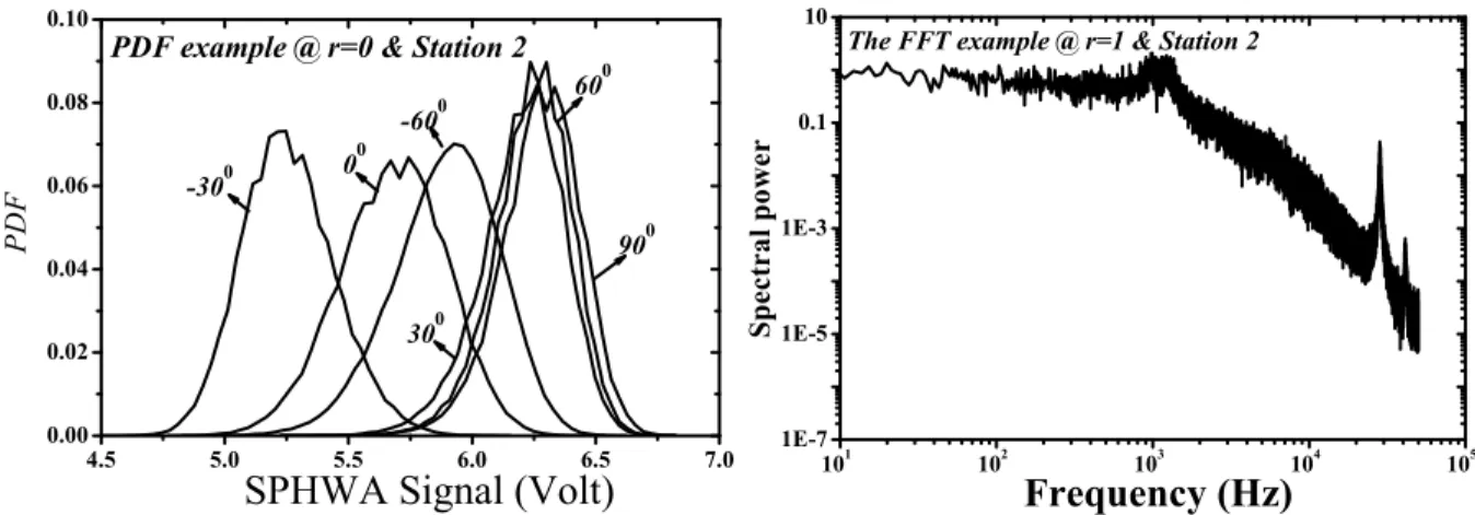
Kurosaka, Chu and Kuroda [41–43] from the University of Tennessee explained the VT with the phenomenon of acoustic streaming. They focused their research on the fundamental functions of ordered/disordered turbulence and found a relationship between the acoustic resonance frequencies and the forced vortex motion frequency. They proposed that the energy separation inside the RHVT is due to the damping of the acoustic streaming along the axis of the tube towards the hot exhaust. In Chapter 6 the frequencies found from the spectral analysis on the samples taken by the hot-wire anemometry also have these relationships and indicate the existence of the acoustic phenomena.

1.2.2.5 Secondary circulation model

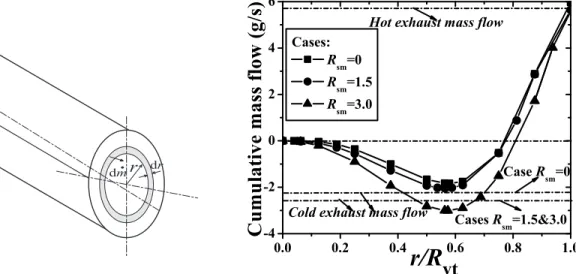
Ahlborn [61, 78] proposed a so-called secondary circulation model based on his experimental results. He found that the cumulative mass flow over the cross section of the vortex tube in the cold end direction is larger than the cold exhaust flow, which implies the existence of a secondary circulation flow in the VT. With this secondary circulation model, the RHVT can be considered as a classical refrigeration device and the secondary circulation flow can be thought as a classical cycle [78].

The secondary flow pattern has also been noted experimentally by Linderstrom-Lang [23, 79], Fulton [66], Scheper [67], Ahlborn [61] and Gao [62], and numerically explained by Cockerill [22], Frohlingsdorf [80], Gutsol [81] and Aljuwayhel [82]. The main difference among all these secondary flow patterns is whether the secondary flow is a closed cycle or not. Linderstrom-Lang, Fulton, Scheper and Cockerill suggested it as an open cycle, while Ahlborn, Gao, Gutsol, Frohlingsdorf and Aljuwayhel suggested a closed cycle. More detailed analysis on the secondary circulation model is discussed in later Chapters. We have chosen to modify this secondary circulation model in this thesis, see Chapter 2.

In summary, as pointed out by van Deemter [73] and Gutsol [63] most of these theories can only either explain their own works and could not match with the others, or be used for qualitative analysis only. This indicates also that the above theories are incomplete. The above mentioned theories point out two directions of theoretical research, which gives hints for further investigations. One is focussing on thermodynamics (compression and expansion), turbulent flow, viscous friction, internal heat transfer, and acoustics. The other one is con-cerning the flow pattern, like secondary circulation. The further analysis of these two aspects form the main body of this thesis.

1.3 Preview of this thesis

In the Low Temperature group at the TU Eindhoven, research is focused on new cooling technologies and their applications. The pulse-tube cryocooler is the main research theme of the group. Another research subject is thermoacoustics. A common property of pulse-tube cooler, thermoacoustic cooler and Ranque-Hilsch vortex pulse-tube is that these have (almost) no moving parts. Furthermore the incomplete understanding of the physical mechanisms occurring in the tube are also a challenge to start working on this subject. This thesis starts research in the RHVT direction for the Low Temperature group.

(17)

1.3 References 9

As discussed in Section 1.2, in the past 70 years, the history follows the pattern of initial enthusiasm, then apathy, and later renewed interest. After Hilsch presented his work, the investigations of RHVT were starting to become prosperous and interested many researchers due to the magical phenomena, sometimes referred to as Maxwell’s demons, occurring in the vortex tube. But due to the inefficient operation, interest in the VT died down during the 1970s. In the 1980s, researchers in the former USSR showed renewed interest and introduced it to China as well. Now in some universities, the RHVT system is a teaching example in thermodynamics lectures. In this thesis we perform fundamental investigations on the RHVT system (to measure the turbulence and the acoustics inside the system). This includes the design of the RHVT system, design and calibration of the measurement techniques and the analysis of the experimental results.

First of all, in Chapter 2, the theoretical analysis of the RHVT system based on the thermodynamic laws is introduced. The secondary circulation model from Ahlborn [78] is introduced. The comments on this model is given in order to further modify it. The modified relationships include vortex chamber geometrical effects. After that, the thermal efficiencies of the RHVT system are defined.

In Chapter 3 the measurement techniques and the calibrations are explained in detail. Here a special designed Cylinder type Pitot tube is used for the pressure measurements, a thermocouple is used for the temperature measurements and a single probe Hot-wire anemom-etry (SPHWA) is used for the turbulence and the velocity measurements. Then in Chapter 4 the design and investigation of a small RHVT system are described to get the first impression of these techniques. It shows that the designed measurement techniques operate very well and the accuracies of these techniques are acceptable. Comparison of the results from this small RHVT system and the work of others is presented. The thermal efficiencies of the small system are calculated, which shows that the efficiencies are lower than 5%. With the calculated cumulative mass flow over the cross sections, a secondary circulation flow is found experimentally.

In Chapter 5 the design of the inlet nozzle is introduced based on gas dynamical anal-ysis. The influences of the operation parameters (inlet pressure, inlet mass flow) and the geometrical parameters (length of nozzle, inlet and exhaust diameters of the nozzle) on the exhaust Mach number, the exhaust momentum and the exhaust pressure are investigated. In Chapter 6, the design of a larger system and the influence of the different components on the performance are discussed, and an optimized system is chosen for further analysis. All the experimental results, based on different techniques, are sampled individually. At the end the velocity, pressure and temperature mappings are shown based on the results from three techniques. In Chapter 7, the thesis is summarized and conclusions are formulated.

References

[1] M.G. Ranque. Experiences sur la detente avec production simultanees dun echappement dair chaud et dun echappement dair froid. J. de Physique et de Radium, 7(4):112–115, 1933.

[2] R. Hilsch. The use of the expansion of gases in a centrifugal field as cooling process. Rev. Sci. Instrum., 18(2):108–113, 1947.

(18)

10 Introduction

[3] L. Khodorkov, N.V. Poshernev, and M.A. Zhidkov. The vortex tube—a universal device for heating, cooling, cleaning, and drying gases and separating gas mixtures. Chemical and Petroleum Engineering, 39(7-8):409–415, July 2003.

[4] Exair.com. http://www.exair.com/vortextube/vt page.htm.

[5] R. Ebmeier, S. Whitney, S. Alugupally, M. Nelson, N. Padhye, G. Gogos, and H.J. Viljoen. Ranque-Hilsch Vortex Tube thermocycler for DNA amplification. Instrumentation Sci-ence and Technology, 32(5):567 – 570, 2004.

[6] R.F. Boucher and J.R. Tippetts. Vortex-tube-driven thermo-electricity. In Sixth tri-ennal international symposium on Fluid Control, Measurement and Visualization, 6th, Sherbrooke, Canada, Paper 50, August 2000.

[7] Method of natural gas liquefaction. Russia patent No. 2202078 C2, April 2003.

[8] R. Westley. Vortex tube performance data sheets. Cranfield College Note 67, College of Aeronautics, 1957.

[9] R. Westley. A bibliography and survey of the vortex tube. Cranfield College Note 9, College of Aeronautics, 1954.

[10] Y. Soni. A parameteric study of the Ranque-Hilsch tube. PhD dissertation, University of Idaho Graduate School, U.S.A., Oct. 1973.

[11] K.G. Hellyar. Gas liquefaction using a Ranque-Hilsch vortex tube: Design criteria and bibliography. Report for the degree of Chemical Engineer, September 1979.

[12] C.U. Linderstrom-Lang. On gas separation in Ranque-Hilsch vortex tubes. Z. Natur-forschg., 22(a):835–837, April 1967.

[13] J. Marshall. Effect of operating conditons, physical size and fluid characteristics on the gas separation performance of a Linderstrom-Lang vortex tube. Int. J. Heat Mass Transfer, 20:227–231, 1977.

[14] K.T. Raterman, M. Mckellar, A. Podgomey, D. Stacey, and T. Turner. A vortex con-tactor for carbon dioxide separations. In First National Conference on Carbon Seques-tration. National Energy Technology Laboratory, U.S.A., http://www.netl.doe.gov/ publications/proceedings/01/carbon seq/7b3.pdf, May 2001.

[15] M.R. Kulkarni and C.R. Sardesai. Enrichment of Methane concentration via separation of gases using vortex tubes. J. Energy Engrg, 128(1):1–12, April 2002.

[16] N.V. Poshernev and I.L. Khodorkov. Natural-gas tests on a conical vortex tube (CVT) with external cooling. Chemical and Petroleum Engineering, 40(3-4):212–217, March 2004.

[17] H. Takahama, H. Kawamura, S. Kato, and H. Yokosawa. Performance characteristics of energy separation in a steam-operated vortex tube. Int. J. Engng Sci., 17:735–744, 1979. [18] R.L. Collins and R.B. Lovelace. Experimental study of two-phase propane expanded through the Ranque-Hilsch tube. Trans. ASME, J. Heat Transfer, 101:300–305, May 1979.

(19)

1.3 References 11

[19] R.T. Balmer. Pressure-driven Ranque-Hilsch temperature separation in liquids. Trans. ASME, J. Fluids Engineering, 110:161–164, June 1988.

[20] M.G. Ranque. Method and apparatus for obtaining from a fluid under pressure two currents of fluid at different temperatures. US Patent No. 1952281, March 1934.

[21] C.D. Fulton. Comments on the vortex tube. J. ASRE Refrigerating Engng, 58:984, 1950. [22] T. Cockerill. Ranque-Hilsch vortex tube. Master thesis, University of Cambridge, 1995. [23] C.U. Linderstrom-Lang. Studies on transport of mass and energy in the vortex tube— The significance of the secondary flow and its interaction with the tangential velocity distribution. Riso report, Denmark, September 1971.

[24] R. Westley. Optimum design of a Vortex Tube fpr achieving larger temperature drop ratios. Cranfield College Note 30, College of Aeronautics, 1955.

[25] H. Takahama and K. Kawashima. An experimental study of vortex tubes. Research, 1960. [26] H. Takahama. Studies on vortex tubes (1) experiments on efficiency of energy separation

(2) on profiles of velocity and temperature. Bulletin of JSME, 8(31):433–440, 1965. [27] H. Takahama and N. Soga. Studies on vortex tubes (2nd report): Reynolds number. the

effects of the cold air rate and the partial admission of nozzle on the energy separation. Bulletin of JSME, 9(33):121–130, 1966.

[28] H. Takahama and etc. Studies on vortex tubes (3rd report): Variations of velocity, temperature and energy with axial distance, the mechanism of energy separation. Bulletin of JSME, 235:503–510, 1966.

[29] H. Takahama and H. Yokosawa. An experimental study of vortex tubes(where the vortex chamber includes a divergent tube). Research, 1981.

[30] H. Takahama and H. Yokosawa. Energy separation in vortex tubes with a divergent chamber. Trans. ASME, J. Heat Transfer, 103:196–203, May 1981.

[31] Y.D. Raiskii and L.E. Tunkel. Influence of vortex-tube configuration and length on the process of energetic gas separation. Journal of Engineering Physics and Thermophysics, 27(6):1578 – 1581, December 1974.

[32] B.B. Parulekar. The short vortex tube. The Journal of Refrigeration, 4:74–80, July and August 1961.

[33] A.J. Reynolds. Studies of Rotating fluids a) Plane Axisymmetric Flow, b) Forced Os-cillations in a Rotating fluid, c) The Ranque-Hilsch Vortex Tube. PhD dissertation, University of London, September 1960.

[34] A.I. Gulyaev. Investigation of conical vortex tubes. Journal of Engineering Physics, 10(3):193–195, 1966.

[35] V.A. Safonov A.I. Borisenko and A.I. Yakovlev. The effect of geometric parameters on the characteristics of a conical vortex cooling unit. Journal of Engineering Physics and Thermophysics, 15(6):1158–1162, 1968.

(20)

12 Introduction

[36] N.V. Poshernev and I.L. Khodorkov. Experience from the operation of a conical vortex tube with natural gas. Chemical and Petroleum Engineering, 39(9-10):602–607, Septem-ber 2003.

[37] L.M. Dyskin. Characteristics of a vortex tube with detwisting of cold flow. Journal of Engineering Physics and Thermophysics, 57(1):756–758, July 1989.

[38] R.W. James and S.A.Mashall. Vortex tube refirgeration. Refrigeration and air condi-tioning, pages 69–88, June 1972. Part 2.

[39] S.A. Piralishvili and V.M. Polyaev. Flow and thermodynamic characteristics of energy separation in a Double-Circuit vortex tube—an experimental investigation. Experimental Thermal and Fluid Science, 12:399–410, 1996.

[40] D.W. Guillaume and J.L. Jolly. Demonstrating the achievement of lower temperatures with two-stage vortex tubes. Review of Scientific Instruments, 72(8):3446–3448, August 2001.

[41] M. Kurosaka. Acoustic streaming in swirling flow and the Ranque-Hilsch (vortex-tube) effect. J. Fluid Mech., 124:139–172, 1982.

[42] J.G. Chu. Acoustic streaming as a mechanism of the Ranque-Hilsch effect. PhD disser-tation, University of Tennessee, Knoxville, Dec. 1982.

[43] H. Kuroda. An experimental study of temperature separation in swirling flow. PhD dissertation, University of Tennessee, Knoxville, Dec. 1983.

[44] Arizona Vortex Tube Manufacturing Company. http://www.arizonavortex.com/ vortextubes.htm.

[45] AirTX The Air Research Technology Company. http://www.airtxinternational. com/catalog/vortex tubes.php.

[46] ITW Air management. http://www.itw-air.com/index.php. [47] ITW Vortec. http://www.vortec-nl.com/.

[48] Newman Tools Inc. http://www.newmantools.com/vortex.htm.

[49] Vortexair.biz. http://www.vortexair.biz/Cooling/SPOTCOOLPROD/spotcoolprod. htm.

[50] R. MacGee Jr. Fluid action in the vortex tube. J. ASRE Refrigerating Engng, 58:974–975, 1950.

[51] J.E. Lay. An experimental and analytical study of vortex-flow temperature separation by superposition of spiral and axial flow, part II. Trans. ASME J. Heat Transfer, 81:213– 222, Aug. 1959.

[52] M. Sibulkin. Unsteady, viscous, circular flow part 3. application to the Ranque-Hilsch vortex tube. J. Fluid Mech., 12:269–293, 1961.

(21)

1.3 References 13

[53] J.L. Smith Jr. An experimental study of the vortex in the cyclone separator. Trans. ASME, J. B. Engng, 84:602–608, Dec. 1962.

[54] J.L. Smith Jr. An analysis of the vortex flow in the cyclone separator. Trans. ASME, J. B. Engng, 84:609–618, Dec. 1962.

[55] W. A. Scheller and G. Martin Brown. The Ranque-Hilsch vortex tube. Fluid Mechanics in Chemical Engineering, 49(6):1013–1016, 1957.

[56] J.E. Lay. An experimental and analytical study of vortex-flow temperature separation by superposition of spiral and axial flow, part I. Trans. ASME J. Heat Transfer, 81:202–212, Aug. 1959.

[57] J.P. Holman and G.D. Moore. An experimental study of vortex chamber flow. Trans. ASME, J. B. Engng, 83:632–636, Dec. 1961.

[58] M. Sibulkin. Unsteady, viscous, circular flow part 1. the line impulse of angular momen-tum. J. Fluid Mech., 11:291–308, 1961.

[59] M. Sibulkin. Unsteady, viscous, circular flow part 2. the cylinder of finite radius. J. Fluid Mech., 12:148–158, 1961.

[60] A.J. Reynolds. A note on vortex-tube flow. J. Fluid Mech., 14:18–20, 1962.

[61] B. Ahlborn and S. Groves. Secondary flow in a vortex tube. Fluid Dynamics Research, 21:73–86, 1997.

[62] C.M. GAO, K.J. Bosschaart, J.C.H. Zeegers, and A.T.A.M. de Waele. Experimental study on a simple Ranque-Hilsch vortex tube. Cryogenics, 45(3):173, 2005.

[63] A. Gutsol. The Ranque effect. Physics-Uspekhi, 40(6):639–658, 1997.

[64] A.I. Leont’ev. Gas-dynamic methods of temperature stratification (a Review). Fuild Dynamics, 37(4):512–529, 2002.

[65] B. Ahlborn, J.Camire, and J.U. Keller. Low-pressure vortex tubes. J. Phys. D: Appl. Phys., 29:1469–1472, 1996.

[66] C.D. Fulton. Ranque’s tube. J. ASRE Refrigerating Engng, 58:473–479, 1950.

[67] G.W. Scheper. The vortex tube–internal flow data and a heat transfer theory. J. ASRE Refrigerating Engng, 59:985–989, 1951.

[68] F. Kreith and D. Margolis. Heat transfer and friction in turbulent vortex flow. Flow, Turbulence and Combustion, 8(1):457 – 473, January 1959.

[69] R.Z. Alimov. Flow friction and heat and mass transfer in a swirled flow. Journal of Engineering Physics and thermophysics, 10(4):251 – 257, April 1966.

[70] A.J. Reynolds. On the dynamics of turbulent vortical flow. Z. angew. Math. Phys., 12:149–158, 1961.

(22)

14 Introduction

[72] R.G. Deissler and M. Perlmutter. Analysis of the flow and energy separation in a turbu-lent vortex. Int. J. Heat Mass Transfer, 1:173–191, 1960.

[73] J.J. van Deemter. On the theory of the Ranque-Hilsch cooling effect. Appl. Sci. Res., 3:174–196, 1951.

[74] W.S. Lewellen. A solution for three-dimentional vortex flows with strong circulation. J. Fluid Mech., 14:420–432, 1962.

[75] Q.H. Wu. The internal process analysis and the experimental investigation on the Ranque-Hilsch vortex tube. Master thesis, Xi’an Jiaotong University, Xi’an, China, 1991.

[76] J.B. Yang. Mathematical model of vortex tube and experimental study of optimizing performance parameters in vortex tube. Master thesis, Xi’an Jiaotong University, Xi’an, China, 1991.

[77] Y.B. Zhang. The theoretical and experimental study on vortex tube. Master thesis, Xi’an Jiaotong University, Xi’an, China, 1993.

[78] B. Ahlborn and J.M. Gordon. The vortex tube as a classic thermodynamic refrigeration cycle. J. Appl. Phys., 88(6):3645–3653, 2000.

[79] C.U. Linderstrom-Lang. Gas separation in the Ranque-Hilsch vortex tube model calcula-tions based on flow data. Riso report, Denmark, June 1966.

[80] W. Frohlingsdorf. Unterschungen zur kompressiblen Str¨omung und Energietrennung im Wirbelrohr nach Ranque und Hilsch. PhD dissertation, Ruhr-Universitat-Bochum, 1997. In German.

[81] A. Gutsol and J.A. Bakken. A new vortex method of plasma insulation and explanation of the Ranque effect. J. Phys. D: Appl. Phys., 39:704–711, 1998.

[82] G.F. Nellis N.F. Aljuwayhel and S.A. Klein. Parametric and internal study of the vortex tube using a cfd model. International Journal of Refrigeration, 28(2):442–450, 2005.

(23)

Chapter 2 Theoretical analysis of the RHVT

Since the 1930s, the mechanism of the energy separation inside the RHVT system has puzzled researchers. Even now, there is no clear theory that can explain the phenomenon completely. In this chapter, the thermodynamical laws are applied to the RHVT system itself. With these laws, the relationships between the entrance and exhaust gas properties and the maximum pressure ratio in the system have been found. The secondary circulation model proposed by Ahlborn [1, 2], is named here the “original secondary circulation model” (OSCM). In this model, Ahlborn applied some assumptions and some ideas which are pointed out in this Chapter. Here, the secondary circulation model is modified. We will call it the “modification of Ahlborn’s model” (MAM). The chamber influence is considered and the compressible flow analysis (gas dynamics) is applied in the analysis of the inlet nozzle. The comparison between the two models shows that MAM agrees better with the measurement than OSCM. At the end, the thermal efficiencies are defined, analyzed, and derived as functions of the inlet and exhaust gas properties.

2.1 Thermodynamical analysis of the RHVT system

The following symbols for the geometric parameters are defined: Dvc is the inner diameter

of the vortex chamber, Dvtis the inner diameter of the vortex tube, Dce the diameter of the

cold exhaust orifice, Dcr is the critical diameter. Inside the vortex chamber, Dcr denotes the

position where the azimuthal velocity changes from the solid body rotation motion to the potential vortex motion, while inside the vortex tube, Dcr denotes the position where the

axial velocity is zero. In practice, inside the chamber Dcr is the same as Dvt, and inside the

tube, Dcr varies with cross sections.

2.1.1 Introduction

Fig.2.1 shows the control volume considered in the thermodynamical analysis. This control volume is taken as a black box. For the analysis, only the gas properties at the walls, at the inlet and exhaust are of interest, i.e. for the analysis details of the internal process do not need to be considered.

In this system, there are three open boundaries namely Ain, Ahand Ac. The gas properties

on these open boundaries are listed as follows. On Ai: pi, Ti, ρi, Vi, ∗

Hi, with subscript i,

(24)

16 Theoretical analysis of the RHVT i n h c p i n T i n r i n V i n H*_{i n} p c T c r c V c H c * p h T h r h V h H h * Q

.

S

.

i

Figure 2.1: Control volume as a black box for the thermodynamical analysis.

the indexes “in”, “h” and “c” for inlet, hot and cold, respectively. p is the pressure, T the temperature, ρ the density, V the velocity and H the enthalpy flux.∗

In the steady flow, mass conservation between inlet flow ( ˙min), cold ( ˙mc) and hot ( ˙mh)

outlet flows reads

˙

min= ˙mh+ ˙mc (2.1)

With ˙mc the cold exhaust mass flow, expressed as ε ˙min, and ˙mh the hot exhaust mass flow,

expressed as (1 − ε) ˙min, obtained

˙

min= (1 − ε) ˙min+ ε ˙min (2.2)

where ε is the cold fraction. Its conventional definition is ε = m˙c

˙ min

. (2.3)

2.1.2 The first law of thermodynamics

Neglecting the velocity contribution and the potential energy, the first law of thermodynamics reads [3] ˙ U =X k ˙ Qk+ X k ∗ Hk− X k pkV˙k+ P (2.4)

where U is the internal energy of the system, and ˙U is the rate of change of the internal energy. The internal energy is only state dependent. In the analysis, the system is considered as steady, and ˙U = 0. ˙Qk are heat flows at the various regions of the boundary. If heat flows

from outside into the system, it is counted as positive. The RHVT system is assumed to be insulated, so ˙Qk = 0.

∗

H is the enthalpy flow into the system defined as H =∗ nh∗ m = ˙mh.

Because the openings are large, the velocities at these openings are much lower than the sound speed, so the velocity term in these enthalpy flows can be neglected. In that case, for a calorically perfect gas the specific enthalpy depends linearly on the temperature

h = cpT ,

here cp is the specific heat at constant pressure, is constant. In Eq. 2.4 ˙Vk is the rate of

(25)

2.1 Thermodynamical analysis of the RHVT system 17

this term is zero. P takes into account all other forms of work done on the system by the environment.

Applying the first law on the system shown in Fig. 2.1, it follows that 0 = ˙min[cpTin− (1 − ε)cpTh− εcpTc] , or Tin− (1 − ε)Th− εTc= 0 . (2.5) Taking ∆Th= Th− Tin, ∆Tc= Tc− Tin and ∆Thc= Th− Tc,

the following relationships can be derived,

Tin= (1 − ε)Th+ εTc

ε∆Tc= (ε − 1)∆Th

∆Th= ε∆Thc

∆Tc= −(1 − ε)∆Thc .

(2.6)

These relationships express the inlet and exhaust temperatures as functions of the cold fraction ε.

2.1.3 The second law of thermodynamics

The second law of thermodynamics reads [3] ˙ S =X k ˙ Qk Tk +X k ∗ Sk+ X k ˙ Sik with S˙ik≥ 0 (2.7)

where ˙S is the rate of increase of the entropy of the system. For the RHVT system in the steady state ˙S = 0. Tk represents the temperatures at which the heat flow ˙Qk enters the

system from the outside. S∗krepresents the entropy flow into the system due to matter flowing

into the system, given asS∗k = ˙mksk, where sk is the specific entropy of the matter flowing

into the system. ˙Si are the entropy production rates due to irreversible processes. Each of

the entropy production rates is always positive. The most important irreversible processes in the RHVT system are:

- heat flow over a temperature difference; - mass flow over a pressure difference; - viscous dissipation.

Applying the second law of thermodynamics to the RHVT with ˙Q = 0, gives 0 = S∗in− ∗ Sh− ∗ Sc+ ˙Si ˙ Si= ∗ Sh+ ∗ Sc− ∗ Sin = m˙in[(1 − ε)(sh− sin) + ε(sc− sin)] . (2.8)

(26)

18 Theoretical analysis of the RHVT

With Rmthe specific gas constant. With the ideal gas assumption, the relation for the specific

entropy becomes [3] ds = cp dT T − Rm dp p . (2.9)

Integrating the above equation from state 1 to state 2, gives s2− s1 = cpln T2 T1 − Rm lnp2 p1 (2.10) Substituting Eq. 2.10 into Eq. 2.8 and assuming pc= ph= pa(pa is the ambient pressure),

we have ˙ Si= m˙in[(1 − ε)(sh− sin) + ε(sc− sin)] = m˙in h (1 − ε)(cpln_TT_inh − Rmln_pp_inh) + ε(cpln_TT_inc − Rmln_pp_inc) i = m˙inRm(_Γ1 lnT 1−ε h Tcε Tin − ln p1−ε_h pε c pin ) = m˙inRm(_Γ1 lnT 1−ε h Tcε Tin − ln pa pin) ≥ 0 (2.11) where γ = cp/cv and Γ = γ − 1 γ = Rm cp . From Eq. 2.11, we have

1 Γln T_h1−εTε c Tin − ln pa pin ≥ 0 T_h1−εT_cε= T∗ sm≥ Tin(_pp_ina)Γ (2.12) here T∗

smis the temperature assumed to be Th1−εTcε. When it equals to Tin(_pp_ina)Γ, which is the

temperature after the isentropic expansion process from Tin and pin to the pressure pa.

If the process in the system is reversible, then Eq. 2.12 becomes T_h1−εT_cε = T∗

sm= Tin(

pm

)Γ. (2.13)

In case of an irreversible process, Eq. 2.11 quantifies the entropy production rate ˙ Si= ˙minRm " 1 Γln T_h1−ǫTε c Tin − ln pa pin # = ˙minRm· 1 Γln T∗ sm Tin + lnpin pa ¸ . (2.14) We introduce 1 Γln T∗ sm Tin + lnpin pa = S˙i ˙ minRm = Θir > 0. (2.15)

The factor Θirrepresents the dimensionless entropy generation from the irreversible processes.

Finally, Eq. 2.15 can be written as T∗

sm= eΓΘirTin(

pa

)Γ. (2.16)

Eq. 2.16 can be combined with Eq. 2.6 from the first law via the factor Θir. In this way,

(27)

2.1 Thermodynamical analysis of the RHVT system 19 0.0 0.2 0.4 0.6 0.8 1.0 10 100 1000 10000 C ol d ex ha us t 1.79 1.5 1.0 0 0.5 1.79 1.5 1.0

E

xh

au

st

T

em

pe

ra

tu

re

(

K

)

Cold fraction

0 0.5 H ot e xh au st 300

Figure 2.2: Hot and cold exhaust temperatures as functions of cold fraction ε based on ther-modynamic analysis with the irreversible processes factor Θir at pin= 6 bar, Tin = 300 K, and

pa= 1 bar. The numbers on the curve are the values of the factor Θir.

K, pin = 6 bar, ph = pc = 1 bar. For different cold fractions ε, we obtain the two exhaust

temperatures, as shown in Fig. 2.2.

When Θir = 0, the process inside the RHVT system is reversible. When the cold fraction

is close to zero, in this extreme case, almost all the inlet gas exhausts from the hot side and the temperature at the cold side is absolute zero. The hot exhaust temperature is very close to the inlet temperature. Practically, it is not possible to generate this extremely low temperature.

When the cold fraction is close to one, almost all the gas will escape from the cold side. According to the adiabatic process assumed, the cold exhaust temperature will depend on the pressure drop over the RHVT system, about 170 K. Again because of the first law, the hot exhaust temperature becomes infinite. In practice, the hot exhaust temperature will never be infinite, since the process inside the RHVT system will never be reversible.

For all cases with nonzero Θir, for the cold fraction increasing the hot and cold exhaust

temperatures increase. For a given cold fraction, if Θir increases between zero and ln (pin/pa),

the hot exhaust temperature decreases, while the cold exhaust temperature increases. If Θir < ln (pin/pa), i.e. in the example of Fig. 2.2 for Θir < 1.79, then ln Tsm∗ /Tin < 0

and T∗

sm< Tin, the process inside the RHVT can be thought as an expansion, reversible or

irreversible. Otherwise, Θir ≥ ln (pin/pa), i.e. in the example of Fig. 2.2 Θir ≥ 1.792, then

ln T∗

sm/Tin≥ 0 and Tsm∗ ≥ Tin, so the process could not be thought as an expansion any more,

(28)

2.2 Secondary circulation model by Ahlborn

Since the 1930s, the flow pattern inside the RHVT system has been an important research topic [4–20]. All these works noted the existence of a secondary flow inside the RHVT system. In 1990s, Ahlborn [1,2,21] further explained the existence of the secondary circulation, proved it experimentally, and proposed an Original Secondary Circulation Model (abbreviated as OSCM) to explain the energy separation.

p i n T i n

r

i n V i n p h T h

r

h V h I n n e r s w i r l i n g f l o w P e r i p h e r y s w i r l i n g f l o w p 0 T ₀

r

₀ V ₀ p c n T _{c n}

r

_{c n} V _{c n} p c T c

r

c V c C r o s s v i e w A A ' A - A '

(a) The periphery and inner swirling flows.

S e c o n d a r y c i r c u l a t i o n l o o p P e r i p h e r y l o o p 1 0 5 4 2 ₃ M i x i n g r e g i o n M i x i n g r e g i o n h c A x i a l v e l o c i t y p r o f i l e

(b) The secondary circulation and periphery loops.

Figure 2.3: The secondary circulation model. The numbers “0”∼“5” show the imagined positions where the assumed processes start and end.

(29)

2.2 Secondary circulation model by Ahlborn 21

2.2.1 OSCM by Ahlborn et al., heat exchange model

Fig. 2.3 shows the general principle of the OSCM proposed by Ahlborn. (a) shows that inside the system there exist two swirling flows. One flow swirls to the hot end in the peripherical region, named the peripherical swirling flow. The other flow anti-swirls to the cold exit in the center region, named the internal swirling flow. Both swirling flows generate a high rotating speed vortex motion inside the vortex tube. They also generate two loops (see (b)). One is the gray region shown in the figure, named the secondary circulation (SC) loop, which acts as the refrigerant or working fluid in a normal refrigeration cycle. The other is named the periphery loop, which is an open loop. The gas that exits this loop is renewed by the injected gas. Some gas elements in this loop first pass the peripherical region from the entrance to the hot end, and escape from the hot end. Other gas elements stay in the loop and return axial direction to the cold end in the center, and exit via the cold exhaust. This loop acts as the high and low temperature environments like in a normal refrigeration cycle. Based on this general idea, it is assumed that work is transferred between the inner regions of low pressure and the peripherical regions of high pressure, and that internal energy is transfered between the inner and peripherical regions via the two loops. All these energy transfer processes together are supposed to lead to the energy separation. The OSCM is built on this consideration.

In order to analyze the processes inside the system, we follow the treatment by Ahlborn. Consider Fig. 2.3, in which numbers “0”∼“5” show positions for the processes inside the SC loop (see Ahlborn [2]). The following parts are distinguished:

a) Heat rejection (0→1, 5→1): Near the inlet nozzles, the temperature T0 of the entering

gas element in the periphery loop (0) is lower than the temperature T5of the gas element

in the SC-loop (5). The incoming gas element and the gas element in the SC-loop mix together. The temperature after mixing is T1. Denoting the mass flow by ˙m0 for the

incoming stream, ˙msc for the SC-loop, Ahlborn et al. assume the following enthalpy

balance to hold, neglecting the kinetic energies, ˙

m0(T1− T0) = ˙msc(Tc− T1) , (2.17)

in which temperature T5 has been replaced by the cold gas temperature Tc.

b) Adiabatic deceleration: When following the peripheral circulation towards the hot end, the rotating gas elements at (1) with Mach number Ma,0 decelerate due to friction.

Ahlborn et al. assume an adiabatic deceleration process in which Th = T1(1 +γ − 1

2 M

2

a,0) = T1(1 + ΓX) , (2.18)

(here the notation X = γ/2M2

a,0 has been adopted, following Ahlborn et al.).

c) Heat absorption (h→4, 3→4): The hot gas in the peripherical loop h partly returns to the cold end near the center of the tube with a mass flow ˙mc. There, the hot gas mixes

with the SC-loop, for which the temperature T3 is assumed equal to T1. After mixing,

the temperature becomes Tc. The heat balance is:

˙

msc(Tc− T1) = ˙mc(Th− Tc) . (2.19)

It implies that the hot gas is cooled by mixing with the gas in the SC-loop. Combing Eqs. 2.17 and 2.19 yields, with ε = ˙mc/ ˙m0:

(30)

2.2.2 The normalized pressure ratio X

Ahlborn et al. assume that the vortical motion of the gas in the vortex chamber can be approximated as a solid body rotation with V = Ωvr, V varying from 0 at the axis to

V0 = ΩvRvc at the outer radius Rvc. The pressure distribution then follows the momentum

balance,

∂p ∂r = ρΩ

2

vr . (2.21)

Ahlborn et al. neglect the radial variation of the density, resulting into the following difference between the pressure pc at the center and the pressure p0 at the outer radius

p0− pc= 1 2ρ0Ω 2 vR2vc= 1 2ρ0v 2 0 = 1 2ρ0c 2 0Ma,02 = γ 2p0M 2 a,0. (2.22)

Then, defining a normalized pressure ratio X,

X ≡ p0− pc p0

, (2.23)

the relation between X and M_a,o2 follows from Eq. 2.22,

X = γ 2M

2

a,0, (2.24)

Usually, p0is not known a priori, but will depend on Mach number Ma,0 and inlet pressure

pin. For this relation, Ahlborn et al. incorrectly applied a momentum balance in

incompress-ible flow approximation to find,

γMa,0 ≃

pin− p0

p0

(2.25)

Combination of Eqs. 2.23, 2.24 and 2.25 leads to their expression for the pressure ratio pin/pc τp= pin pc = 2X + 1 1 − X . (2.26)

It can be found that the maximum value of τp is 8 when Ma,0 = 1 and γ = 1.4.

2.2.3 The OSCM model

Instead of solving Eqs. 2.18 and 2.20, Ahlborn et al. present an approximation based on a simplifying assumptions regarding the values of T0 and T1. It is assumed that T0 and T1 are

(31)

note their final expressions [1, 2, 21, 22] Th Tc = 1 +(γ − 1) γ X(ε + 1) = 1 + ΓX(ε + 1) (2.27a) Th Tin = 1 + 6ΓXε 4 + 3ΓX (2.27b) Tc Tin = 1 + 6ΓXε 4+3ΓX 1 + ΓX(ε + 1) (2.27c) ∆Th Tin = Th− Tin Tin = 6ΓXε 4 + 3ΓX (2.27d) ∆Tc Tin = Tc− Tin Tin = 6ΓXε 4+3ΓX − ΓX(1 + ε) 1 + ΓX(1 + ε) (2.27e) X = γ 2M 2 a,0 . (2.27f)

2.2.4 Comments on the model of Ahlborn et al.

Ahlborn et al. have formulated a “physical” model of the RHVT (named “Original Secondary Circulation Model”) by employing its similarity with a heat pump [1, 2]. According to the OSCM, the following remarks should be made:

1. The compressibility of the working fluid is sometimes disregarded, sometimes taken as an essential component. For example, the entrance flow in the nozzle is described in their publication [22] as incompressible, while important phenomena as “choking” in a throat can only be explained with a correct formulation based on compressibility. Furthermore, it is not possible to find the exit Mach number for a nozzle from an integral momentum balance.

2. The kinetic energy of the peripheral fluid and of the fluid in the SC-loop is sometimes taken into account, sometimes not. The arguments are not given. It is correct that the lowest temperature in the vortex tube can be found near the entrance. But this low temperature is a direct consequence of the high kinetic energy. Still, it is assumed that in the mixing region near the entrance (0 →1 for the peripheral flow and 5 → 1 for the flow in the SC-loop) the enthalpy flow remains constant while the kinetic energy is disregarded. But in an overall adiabatic setting this only holds for the stagnation en-thalpies, including the kinetic energies of the mixing fluid. If this would be implemented in the theory we would find Tc= Th= Tin, in other words, the model would fail.

3. Ahlborn et al. assumed the velocity distribution inside the vortex chamber to be a Rankine vortex motion, which is experimentally correct and acceptable. But in their description, they only considered the solid body rotation in the center region of the Rankine vortex motion, and not the potential vortex motion in the peripheral region. If the peripheral region is considered as well, then the parameter X should contain information on the geometry.

4. Let us assume that T0 is adiabatically related to Tin, according to

Tin= T0(1 + γ − 1

2 M

2

(32)

If we substitute T0 from Eq. 2.28 in Eqs. 2.18 and 2.20, and combine this with the

gen-eral energy balance (see Eq. 2.6), we would find Th= Tc= Tin, which is a disappointing

result.

5. It should be concluded that the OSCM from Ahlborn et al. cannot be considered as a satisfactory theoretical model of the flow inside the RHVT, but that its merit is based on its success as an empirical description of the RHVT performance.

2.2.5 Modification of Ahlborn et al.’s model

Based on the above mentioned remarks, the OSCM is modified in the following aspects: (a) The Mach number Ma,0 is calculated based on compressible flow through a throat

p0

= (1 + Γ2Ma,02 )1/Γ . (2.29)

(b) Because in the vortex chamber, the geometry is axi-symmetric and the axial velocity vz

and radial velocity vr are much smaller than vθ and can be neglected, the momentum

equation is simplified to [22] ∂p ∂r ≃ ρv2 θ r . (2.30)

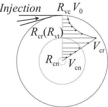
So, the pressure distribution inside the vortex chamber merely depends on the tangential velocity vθ profile. The Rankine velocity profile (see Fig. 2.4) reads [23]

vθ =½ ΩvΓr 0 ≤ r ≤ Rc cr

r Rcr≤ r ≤ Rvc.

(2.31)

Here Γc is the vortex circulation, Ωv is the vortex vorticity. In the vortex chamber,

there are a few radii: one is the chamber radius Rvc; the critical radius Rcr; the vortex

tube radius Rvt; the last one is the radius Rcnnear the center which can be thought as

the same of the cold exhaust orifice radius. Experimentally, Rcrequals Rvt(see Chapter

6). When r = Rvc, the velocity should be the nozzle exit velocity V0. The continuity of

velocity at r = Rcr= Rvt requires Γc/Rcr= ΩvRcr. For the vortex circulation and the

vorticity in Eq. 2.31 we find

Γc = V0Rvc, and

Ωv = V0_RR2vc

cr .

The velocity distribution of Eq. 2.31 can be substituted in the momentum equation 2.30 and integrated. Ahlborn et al. assumed a constant density in the vortex chamber. With the same approximation, the following pressure distribution is obtained

p(r) = ( c1+1₂ρΩ2vr2 (0 ≤ r ≤ Rcr) c2−ρΓ 2 c 2r2 (Rcr≤ r ≤ Rvc) (2.32) where c1 and c2 are to be determined from the boundary conditions

(33)

R

_{v c}

V

₀

V

_{c r}

R

_{c n}

R

_{c r}

( R

_{v t}

)

V

c n

I n j e c t i o n

Figure 2.4: Rankine velocity distribution in the vortex chamber: Rvc is the radius of the vortex

chamber; normally the maximum velocity inside the vortex chamber occurs when the radius reaches the vortex tube radius, so Rcr is equal to the vortex tube radius Rvt (see Chapter 6).

Rcn is close to the center of the vortex chamber.

and continuity of pressure at r = Rcr.

Finally we obtain p0− pc= p0 γ 2M 2 a,0 2R2_vc_{− R}2_cr R2 cr . (2.33)

So the normalized pressure ratio X reads

X = γ₂M_a,02 2R2vc−R2cr

R2

cr ,

M_a,02 = _γ2X′ _,

(2.34)

so X′ _{varies from 0 to 0.7 for nitrogen. At the same time, we introduce a parameter}

τR = Rcr Rvc = Rvt Rvc . (2.35)

τR is dependent on the geometry of the vortex chamber and varies from 0 to 1. X′ and

X have the following relationship

X′ ₌ τR2

2 − τ2 R

X, (2.36)

so X is the normalized pressure ratio, is dependent on these pressures, in other words, it is dependent on X′ _{and τ}

(34)

(c) The pressure ratio τp over the vortex tube is computed with Eqs. 2.29 and 2.33 (or

2.34). It reads τp = p_pin_c = (1+Γ2Ma,02 )1/Γ 1−γ2Ma,02 2R2_vc−R2_cr R2_cr = (1+Γ2M 2 a,0)1/Γ 1−γ2Ma,02 (_{τ 2}2 R−1) = (1+0.2Ma,02 )7/2 1−0.7M2 a,0(_{τ 2}2 R−1) , (2.37)

when Ma,0= 0, τp = 1. It can be found that when τR= 1 (the case used by Ahlborn et

al.) in order to achieve “choking” condition at the exhaust of the nozzle, the pressure ratio τp should be around 6.3 which is much less than what is found from Ahlborn et

al.’s model. The reason for this difference is that Ahlborn et al. applied an incorrect incompressible momentum balance to the nozzle flow.

0.0 0.2 0.4 0.6 0.8 1.0 0.0 0.2 0.4 0.6 0.8 1.0

X

M

_a,0 1.0 0.8 0.6 0.4 R=0.2

Figure 2.5: Normalized pressure ratio X (= (p0−pc)/p0) vs. Ma,0for different τR(= Rvt/Rvc).

Fig. 2.5 shows the relation between the normalized pressure ratio X and the Mach number Ma,0 for different ratios τR. When τR = 1, the maximum normalized pressure

ratio X is 0.7 which is the same as obtained by Ahlborn. It should be noted that the model only gives reasonable results when the density difference in the vortex chamber is sufficiently small, i. e. X < 0.5.

(d) We shall adopt a similar enthalpy balance as derived by Ahlborn et al., i.e. (Eqs. 2.17, 2.19 and 2.20)

˙

m0(Tc− T1) = ˙mc(Th− Tc),

or

(35)

We will not make use of of Eq. 2.18. The temperature T0 is adiabatically connected to

the inlet temperature Tin, assuming the stagnation enthalpy to be a conserved quantity

Tin= T0(1 + Γ2Ma,02 ) = T0(1 + ΓX′) . (2.39)

Combination of Eq. 2.38 and 2.39 yields, Th Tc = 1 +1 ε T1 Tc − 1 ε(1 + ΓX′₎ Tin Tc . (2.40)

Further, we shall adopt the assumption of Ahlborn et al. that T1is approximately equal

to Tc. We then find, Th Tc ≃ 1 + 1 ε− 1 ε(1 + ΓX′₎ Tin Tc . (2.41)

Solving Eq. 2.6 from energy conservation and Eq. 2.41, the relationships for the modified Ahlborn et al.’s model are obtained

Th Tc = 1 + ΓX ′ 1 + εΓX′ (2.42a) Tc Tin = 1 + εΓX′ 1 + ΓX′ (2.42b) Th Tin = 1 + εΓX ′ 1 + ΓX′ (2.42c) ∆Th Tin = εΓX ′ 1 + ΓX′ (2.42d) ∆Tc Tin = (ε − 1)ΓX ′ 1 + ΓX′ (2.42e) X = γ 2M 2 a,0( 2 τ2 R − 1), and X′ = τ 2 R 2 − τ2 R X . (2.42f)

It should be noted that also the modified Ahlborn et al.’s model (MAM) has to be con-sidered as an empirical model, based on rather crude approximations and on questionable assumptions.

2.2.6 Comparison of the computations with OSCM and MAM

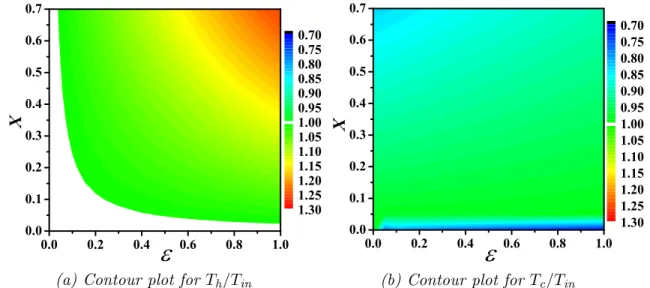
Fig. 2.6 shows the results calculated with Eq. 2.27 from the analysis of Ahlborn et al.. Fig. 2.7 shows the results calculated with Eq. 2.42 from this work. As shown in these figures, when the cold fraction ε and X or X′ increases, the temperature ratio Th/Tin increases as

well. For both cases, Th/Tin can be about 1.25 in the OSCM, and only about 1.15 with

MAM. When X < 0.1, the temperature ratio Tc/Tinvaries very rapidly from 0.98 to 0.8 with

OSCM. When X > 0.1, if X increases and ε decreases, Tc/Tin decreases from 0.98 to 0.84.

Its minimum value for OSCM is about 0.8. With MAM, derived in this work, if X increases and ε decreases, Tc/Tin decreases from about 1.0 at X

′

about 0 and ε about 1 to 0.84 at X′ about 0.7 and ε about 0. So it shows that the ranges of the temperature ratios predicted with OSCM are always wider than those with MAM. It also shows that when X = 0, which means that p0 = pc, there is no flow inside the system, the temperature ratios Tc/Tin and Th/Tin

must be unity. In the OSCM, the temperature ratio Tc/Tin can be 0.72 (when X < 0.05),

12- VORTEX TUBE

Experimental Study

on

the Ranque-Hilsch Vortex Tube

PROEFSCHRIFT

Chengming Gao

Contents

Chapter 1

Introduction

1.1

Background

1.2

The state of the art

1.3

Preview of this thesis

References

Chapter 2

Theoretical analysis of the RHVT

2.1

Thermodynamical analysis of the RHVT system

.

.

E

xh

au

st

T

em

pe

ra

tu

re

(

K

)

Cold fraction

2.2

Secondary circulation model by Ahlborn

r

r

r

r

r

R

v c

V

0

V

c r

R

c n

R

c r

( R

v t

)

V

c n

I n j e c t i o n

X

M

_{v c}

₀

_{c r}

_{c n}

_{c r}

_{v t}