2 The Method of Moments

CHAPTER

2

The Method of Moments

Abstract- In this chapter, the Method of Moments is introduced and used

in conjunction with integral equations to develop a simple and efficient numerical procedure for treating problems of scattering by arbitrarily shaped objects. This involves the discretization of continuous equations into matrix form. Crucial to the numerical formulation is the choice of a set of special domain type or sub-domain-type basis functions and testing functions. The specific discretization places a limit on the accuracy of a numerical result for a fixed number of basis and testing functions and determines whether or not the numerical result will converge to the exact solution as the number of basis and testing functions is increased.

2.1

INTRODUCTION

The advent of high-speed computers has opened a new realm in the study of electromagnetics and has made it practicable to successfully study a wide variety of problems. The basic idea is to reduce a functional equation to a matrix equation, and then solve the matrix equation by known techniques. Of the many approaches available for the formulation of the electromagnetic radiation and scattering problems, the integral equation method appears to be the one most conveniently adaptable to computer solution. It should be pointed out that the conventional magnetic field integral equation (MFIE), which is found to be very suitable and preferable for solid surface scatteres, is not convenient for electrically thin antennas or scatterers. One therefore

uses an alternative form of the integral equation, the electric field integral equation (EFIE), for such geometry. The above difference in the use of the type of integral equation is an important feature that distinguishes the treatment of thin and solid surface structures.

There are a number of approaches available to the numerical analyst for reducing the integral equation for computer processing. One of most important and commonly used numerical techniques is the Method of Moments [1] [10].

An integral equation can be written symbolically as ,

L f =g (2.1)

where L is a continuous, linear operator such as the integral operators, f is the

unknown to be determined, and g represents a known excitation. The linear operator L

maps a function in its domain (such as f ) to a function in its range (such as g ). As a

general rule the domain and range are different linear spaces. If a unique solution

exists, it is given by f =L g−1 where L−1 is the inverse operator. In practice to

determine L−1 is very difficult and it is more convenient to use numerical techniques.

The equation (2.1) can be transformed into a matrix equation by expanding the

unknown in terms of a set of basis functions

φ

_n

, n n n

f =

∑

α φ

(2.2)

where

α

_n are the unknown expansion coefficients. The matrix equation of the solution,

in the Moment Method, is obtained by applying a inner product to (2.2) after defining a set of testing or weighting functions. It is convenient to introduce the notion of inner product, which is a scalar quantity satisfying the following properties

* * , , , , , , , , 0 if 0, , 0 if 0, f g g f f g h f h g h f f f f f f

α

β

α

β

= + = + > ≠ = = (2.3)

where α and

β

are scalars, f g h, , are functions, and * indicates the complex conjugate. Two functions, f and g, are orthogonal if their inner product is zero, i.o.:

, 0,

f g = (2.4)

In a similar fashion, functions

{ }

φ

_n in an inner product space form an orthogonal set if

, 0.

n m

φ φ = (2.5)

The set

{ }

φ_n is said to be complete if the zero function is the only function in the inner product space orthogonal to each member of the set. A set

{ }

φ_n that is both complete and orthogonal is said to be a basis and can be used to represent any function f in the inner product space in the sense that

0,

n n n

f −

∑

α φ = (2.6)

where

{ }

α_n are scalar and unique coefficients

, . , n n n n f

φ

α

φ φ

= (2.7)

In practice, we are forced to project the functions of interest onto a finite-dimensional subspace of the original inner product space. In the subspace, the basis is truncated to the form

{

φ φ

₁, _2,KK

φ

_n

}

and f is given by

1 . N N n n n f f

α φ

= ≅ =

∑

(2.8)

The

{ }

α_n are chosen to minimize the distance between f and its truncated representation f N

(

N

)

N .

d f − f = f − f (2.9)

It is minimized if

{ }

α_n are chosen to make the error orthogonal to the N-dimensional basis

, N 0, 1, 2, , .

n f f n N

φ

− = = _K (2.10)

This is known as an orthogonal projection.

2.2

THE METHOD OF MOMENTS

The Method of Moments (MoM) is a widely used numerical technique for electromagnetic problems. In this method, one solves the problem by first formulating it into an operator equation, usually of the integral or integro-differential type, that has a finite spatial domain. The unknowns are then expanded in terms of a finite number of well-chosen basis functions; this process is called discretization. A set of matrix equations is then generated by performing a scalar product between the operator equation and a set of selected weighting functions.

As in the preceding section, an approximate solution of the linear equation (2.1) can be obtained in the form

1 , N N n n n f

α φ

= ≅

∑

(2.11)

where

{ }

φn are called basis functions defined on the domain of L and

{ }

αn are scalars

to be determined. Substituting (2.11) in (2.1) and using the linearity of L the equation can be rewritten as

( )

1 , N n n n L g

α

φ

ε

= − =

∑

(2.12)

where ε is called residual error.

This residual is forced to be orthogonal to a set of testing functions

{ }

w_m in order to obtain a set of linear equations. This means w_m,ε = . 0

The result is , , . n m n m n w L w g

α

φ

=

∑

(2.13)

This set of equations can be posed in a matrix form

[ ][ ] [ ]

lmn αn = gm (2.14) Where

[ ]

[ ]

[ ]

1, 1 1, 1 1, 2 2 2, 2, 1 2, 2 , , , , mn n m n _m w g w L w L w g l w L w L g w g

α

φ

φ

α

φ

φ

α

α

⎡ ⎤ ⎡ ⎤ ⎡ ⎤ _{⎢ ⎥ ⎢ ⎥} ⎢ ⎥ _{⎢ ⎥ ⎢ ⎥} =⎢ ⎥ =_{⎢ ⎥} =_{⎢ ⎥} ⎢ ⎥ _{⎢ ⎥ ⎢ ⎥} ⎢ ⎥ ⎣ ⎦ _{⎣ ⎦} ⎢_⎣ ⎥_⎦ K K M _M M M O (2.15)

If the matrix

[ ]

l is non-singular its inverse ⎡ ⎤_{⎣ ⎦}l−1 exists. The

{ }

αn are then given by

[ ]

1

[ ]

mn

n l gm

α

_{⎡ ⎤}−

= ⎣ ⎦ (2.16)

The discretization of continuous equations by the Method of Moments necessarily involves the projection of the continuous linear operator onto finite-dimensional subspaces defined by the basis and testing functions. One of the main tasks in any particular problem is the choice of the

{ }

φ

_n and

{ }

w_m . The

{ }

φ_n should be linearly independent and chosen so that some superposition (2.11) can approximate f

reasonably well. The

{ }

w_m should also be linearly independent. The testing and basis functions used in practice are often not orthogonal sets. This makes it difficult to make firm statements about the convergence of the numerical approximation in equation (2.11) to the exact solution as N → ∞ . In any case, since N is necessarily finite for numerical calculations, the result obtained from (2.11) is always approximate.

The choice of basis and testing functions is the principal issue arising within a Method of Moments implementation. Additional factors affecting the choice of

{ }

φ

n and

{ }

wm

are: the accuracy of the approximate solution, the easy evaluation of matrix elements, the size of the matrix that can be inverted, and the realization of a well-conditioned matrix

[ ]

l .

2.3

BASIS AND TESTING FUNCTIONS

An important step in the MoM is the choice of a set of expanding and weighting functions. Each element of

[ ]

l matrix involves at least two integrations. One integral appears in the linear operator L or better in the original integral equation, and another one is due to the inner product. These integrals cannot be analytically performed. As a result, the computation time required to obtain the

[ ]

l matrix can be considerable. Consequentially, it is necessary to judiciously choose

{ }

w_m and

{ }

φ

_n to reach a good

trade-off between accuracy of solution and computational effort. There are many possible sets of these functions. However, only a limited number are used in practice.

2.3.1 Basis Functions

The basis function can be divided into two general groups. The first group consists of sub-domain functions, which are non-zero only over a part of the domain of the function f . The second class contains entire domain functions that exist over the entire domain of the unknown function.

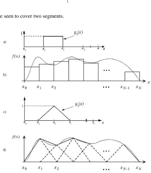
Sub-domain functions are the most commonly used bases. Unlike entire domain bases, they may be used without prior knowledge of the nature of the function that they must represent. The sub-domain approach involves subdivision of the structure into N nonoverlapping segments for a one-dimensional problem, as illustrated in fig 2.1. The basis functions are defined in conjunction with the limits of one or more of the segments. The most common of these basis functions is the piecewise constant, shown in fig 2.1 a. It is defined by

( )

1 1 , 0 otherwise. n n n x x x f x = ⎨⎧ − ≤ ≤ ⎩ (2.17)

Once the associated coefficients are determined, this function will produce a staircase representation of the unknown function, similar to that in figure 2.1 b.

Another common basis set is the piecewise linear functions seen in fig 2.1 c. These are defined by

1 1 1 1 1 1 ( ) 0 elsewhere n n n n n n n n n n n x x x x x x x x x f x x x x x x − − − + + + − ⎧ _{≤ ≤} ⎪ − ⎪ ⎪ − =_⎨ ≤ ≤ − ⎪ ⎪ ⎪ ⎩ (2.18)

and are seen to cover two segments.

Fig. 2.1 Examples of sub-domain basis functions

The resulting representation (fig. 2.1 d) is smoother than that of the piecewise constant, but at the cost of increased computational complexity. Other common bases are piecewise sinusoidal or truncated cosine. Generally, these types of functions are related on a proper meshing of the geometry.

Entire domain basis functions are defined and are non-zero over the entire length of the structure being considered. Thus, no segmentation is involved in their use. A common domain basis set is that of sinusoidal functions where

(

2

)

( ) cos , - . 2 2 n n a x x l l f x x l

π

′ − ⎡ ⎤ = _{⎢ ⎥} ≤ ≤ ⎣ ⎦ (2.19)

The main advantage of entire domain basis functions lies in problems where the unknown function is assumed a priori to follow a known pattern. These types of functions yield a bad convergence of the numerical method and are not versatile but generate a smaller matrix equation than the sub-domain functions. Because we are constrained to use a finite number of functions, entire domain basis functions usually have difficulty in modelling arbitrary or complicated unknown functions.

High Level basis functions are defined on macro domains (several wavelengths size) that include a relatively large number of conventional sub-domains arising in a triangular or rectangular patch modeling of the objects. These type of basis functions lead to a significant reduction in the number of unknowns. Despite entire domain basis functions, high level bases do not pose difficulties in modeling arbitrary or complicated unknown functions.

2.3.2 Testing Functions

Expansion of equation (2.12) leads to one equation with N unknowns. It alone is not sufficient to determine the N unknowns

{ }

α

n . To resolve the N constant unknowns

it is necessary to have N linearly independent equations. This can be accomplished by using the inner product, previously introduced, in conjunction with a set of weight functions. There are different choices for testing functions as fig. 2.2 shows in the second column. One choice can be the Galerkin’s procedure. The Galerkin’s method involves letting the expansion and weighting functions be the same. That is, w_n = .

φ

_n MoM codes based on Galerkin’s method are generally more accurate and rapidly convergent. It has been noted in the previous sections that each term of matrix

[ ]

l

(2.16) requires two or more integrations, at least one to evaluate each L f

( )

n , and one

to perform the inner product. When these integrations are to be done numerically vast amounts of computation time may be necessary. There is a unique set of testing functions that reduce the number of required integrations. This is the set of Dirac delta weighting functions.

The use of Dirac delta for both basis and testing functions is called point matching. It means to enforce the equivalence between the actual function and its approximation only at discrete points. An important consideration when using point matching is the positioning of the N match points. It is important that a match point does not coincide with points where the basis function is not differentiability continuous. This may cause errors in some situations.

Fig. 2.2 Different choices of testing and weighting functions in the MoM

2.4

RWG BASIS FUNCTION

In the preceding paragraphs the problem of discretization has been introduced for one-dimensional problems. In this case, the discretization problem is solved by a segmentation of the domain. This approach is not suitable for surfaces. For modelling

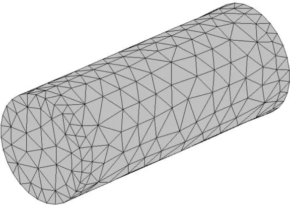
arbitrarily shaped surfaces, planar triangular patch models are particularly appropriate, as shown in fig. 2.3. Triangular patches are capable of accurately conforming to any geometrical surface or boundary. It is important to note that the conventional Method of Moments requires a

λ

10 or

λ

20 discretization. This means that the sides of triangular patches cannot be longer than

λ

10.

Fig. 2.3 Surface modelled by triangular patches

A set of basis functions introduced by Glisson [3] is suitable for use with triangular patch modelling. Each basis function

φ

_n( )r is to be associated on an interior, not boundary, edge of the patch model and defined non-zero on the two triangles attached to that edge (fig. 2.4). These two triangles are indicated by Tn

+

and Tn

−

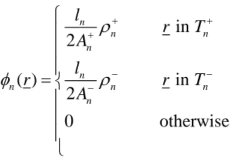
. The plus or minus designation of the triangles is determined by the choice of a positive current reference direction for the nth edge (fig. 2.4), the reference for which is assumed to be from T_n+ to T_n−. The vector basis function associated with the nth edge is defined as

in 2 ( ) in 2 0 otherwise n n n n n n n n n l r T A l r r T A

ρ

φ

ρ

+ + + − − − ⎧ ⎪ ⎪ ⎪ = ⎨ ⎪ ⎪ ⎪ ⎩ (2.20)

where l is the length of the edge, _n A_n± is the area of triangle T_n±, and

ρ

_n± is the distance between a generic point of T_n± and a free vertex of T_n±.

Fig. 2.4 Geometry of triangular patches

The basis function

φ

_n( )r is used to approximately represent the surface current. It has some properties, which make it uniquely suited for this role.

The current has no component normal to the boundary of the surface formed by the triangles T_n±, and hence no line charges exist along this boundary.

The component of current normal to the nth edge is constant and continuous across the edge.

The surface divergence of f r_n( ), which is proportional to the surface charge density associated with the basis element, is:

in , ( ) in , 0 otherwise . n n n n S n n n l r T A l r r T A

φ

+ + − − ⎧ ⎪ ⎪ ⎪ ∇ ⋅ _{= ⎨} ⎪ ⎪ ⎪ ⎩ (2.21)

Sometimes, when the surface is planar and rectangular, a quadrilateral patch modelling is preferred and used with so-called roof-top basis functions.

2.5

SOLUTION OF INTEGRAL EQUATIONS WITH MoM

2.5.1 Testing of the EFIE for Perfect Conductor

A case of particular practical interest is the study of scattering problems of a conducting scatterer using the electrical field integral equation in conjunction with the Method of Moments. Let S denote the surface of an open or closed perfectly conducting scatterer with a unit normal $n . An electric field Eurinc, defined to be the field due to an impressed source in the absence of the object, is incident onS and induces surface currents Jur. If S is open, we regard Jur as the vector sum of the surface currents on the opposite sides of S. In the same way used in the first chapter, we can define the scattering field, using the mixed potential formalism of equations (1.12), as

,

scat

E = −j

ωμ

A− ∇Φ

ur ur

(2.22)

where urA and Φ are the magnetic vector potential and scalar potential, respectively, introduced in the first chapter, and defined as

( )

( ) , 4 1 , 4 jkR S jkR S S e A r J dS R e r dS R

π

ρ

πε

− − ′ = ′ Φ =

∫

∫

ur ur (2.23)

R= − is the distance between an arbitrarily located observation point r and a r r′ source point r′on S and the surface charge density

ρ

_S is related to the surface divergence of Jur through the equation of continuity

.

S J j

ωρ

S

∇ ⋅ = −ur (2.24)

In the same fashion of chapter one, an integral-differential equation for urJ can be derived by enforcing the boundary condition n$×

(

urEinc+uvEscat

)

=0 on S obtaining

(

)

tan tan , on . inc E j Aω r S −ur = − ur− ∇Φ (2.25)

To solve the above EFIE [3] [11] [12], the surface S of the conducting object is first discretized into triangular patches and then RWG basis functions φ_n are used to approximate the current on S as follows

1 , N n n n J I

φ

= =

∑

ur (2.26)

where N is the total number of basis functions, I are the unknowns coefficients to be n

determined. Substitution of the current expansion (2.26) into (2.25) and then application of testing procedures yields an N× system of linear equations which N may be written in matrix form

where

[ ]

Zmn is an N× matrix and N

[ ]

In and

[ ]

Vm are column vectors of length N .

Usually

[ ]

I_n and

[ ]

V_m are referred to as generalized current and voltages vectors, respectively, and

[ ]

Z_mn is referred as a generalized impedance matrix. This matrix has a physical meaning only if an EFIE formulation in the frequency domain is used. The physical interpretation of elements of matrix

[ ]

Z_mn is:

element Z_mn, where n≠ , represents the effect of cell m on cell n which is called m coupling.

element Z represents the self-term. It presents some problems for evaluation because _nn of the singularity of Green’s function when the source point coincides with the observation point. In this case particular shrewdness is used.

The elements of

[ ]

Z_mn and

[ ]

V_m are then given by

, 2 2 , 2 2 c c m m mn m mn mn mn mn c c m m m m m m Z l j A A V l E E ρ ρ ω ρ ρ + − + − + − + − + − ⎡ ⎛ ⎞ ⎤ = _{⎢ ⎜} ⋅ + ⋅ _⎟+ Φ − Φ _⎥ ⎝ ⎠ ⎣ ⎦ ⎛ ⎞ = _⎜ ⋅ + ⋅ _⎟ ⎝ ⎠ ur ur (2.28) where

( )

( )

' , 4 1 , 4 , m m jkR mn n m S jkR mn S n m S c m m e A r dS R e r dS j R R r r μ φ π φ π ωε ± ± − ± ± − + ± ± ± ′ = ′ ′ Φ = − ∇ ⋅ ′ = −

∫

∫

(2.29)

If we approximate the averages of the scalar potential Φ , the vector potential Aur, and the incident field Eurinc over each triangle by their values at the centroids of the triangle, we can bypass the surface integrals of the potentials and reduce the double integrals

over the surface to a single one. The electric field integral equation used until now is expressed in a frequency domain and it has been solved via MoM. It is important to underline that a solution in the frequency domain obtained via factorization or inversion for a given frequency is independent of the exciting source geometry. Thus the induced currents can be obtained for any illuminating field from the product of the inverse matrix and the source vector. The time-domain formulation is, on the other hand, source geometry dependent, but can cover a broad frequency range.

2.5.2 Testing of the PMCHW

In this section, we present a MOM technique for the scattering by three dimensional dielectric bodies of arbitrary shape located in an homogenous medium of infinite extent. The application of the testing procedure (Galerkin’ choice [11] [12] ) to (1.26) yields to

(

)

(

)

(

)

(

)

1 2 1 2 1 2 ' ' 1 2 1 2 1 2 1 2 1 2 , , , , , , , , inc m m m m inc m m m m F F E f j A A f f f A A H f j F F f f f

ω

ε

ε

ω

μ

μ

⎛ ⎞ = + + ∇Φ + ∇Φ + ∇×_⎜ + _⎟ ⎝ ⎠ ⎛ ⎞ = + + ∇Ψ + ∇Ψ − ∇×_⎜ + _⎟ ⎝ ⎠ uuv uuv

uv uuv uuv uuv uuv uuv uuv

uuv uuv

uuv uuv uuv uuv uuv uuv uuv (2.30)

The left hand side term can be expressed as below:

1 1 1 1 , ( ) ( ) 2 2 , ( ) ( ) 2 2 c c

inc inc c inc c

m m

E m m m m

c c

inc inc c inc c

m m H m m m m V E f l E r E r V H f l H r H r

ρ

ρ

ρ

ρ

+ − + − + − + − ⎡ ⎤ = = _⎢ + _⎥ ⎢ ⎥ ⎣ ⎦ ⎡ ⎤ = = _⎢ + _⎥ ⎢ ⎥ ⎣ ⎦ uuv uuv

uv uuv uuv uv uuv uv

uuv uuv

uuv uuv uuv uv uuv uv (2.31)

where ruuv_mc± are the centroids of adjacent patches to the mth testing edge.

The first term in the right hand side part of equation (2.30) can be simplified by evaluating the vector and scalar potentials at centroids ruuv_mc±.

The second term can be simplified as following:

( ) ( )

1 1 , ( ) m m c c m m m m m m m m S T T P f P f dS l PdS PdS l P r P r A − A + − + − + ⎡ ⎤ ⎡ ⎤ ∇ = − ∇ ⋅ = ⎢ − ⎥≅ _⎣ − _⎦ ⎢ ⎥ ⎣ ⎦

∫∫

∫∫

∫∫

uuv uuv (2.32)

and, similarly, the third term with curl operator:

, ( 2 2 m m m m m m m m m m S T T l l X f X f dS X dS X dS A + ρ A + ρ + − + ⎡ ⎤ − ⎡ ⎤

∇×uuv uuv = −

∫∫

∇× ⋅uuv uuv =

∫∫

uuv ⋅ ∇×_⎣ uuv_⎦ +

∫∫

uuv ⋅ ∇×_⎣ uuv_⎦ (2.33) where P and X indicate the magnetic or electric scalar and vector potentials, respectively,

and X is evaluated at centroids. Further simplification can be introduced in (2.33), by changing the vector potential expression:

( )

mc ( ') ' i

(

mc , '

)

( )

'

S

X r ± const Y r G r ± r dS r

∇×uuv uuv =

∫∫

uv v ×∇ uuv v v (2.34)

where Y indicates equivalently the electric or magnetic currents according on the type of potential, Gi is the free-space Green function of region i that can be expressed as:

(

)

(

)

_{( )}

' 3 ( , ') ' ( , ') ' 1 i i jk R c i m c m jk R c c i m m i e G r r R R r r e G r r r r jk R R ± ± − ± ± ± − ± ± _± ± = = − ∇ = − + uuv uv uuv uv uuv uv uuv uv (2.35)

Finally, we obtain a matrix equation form:

JJ JM DD MJ MM Z C Z D Y ⎡ ⎤ = ⎢ ⎥ ⎢ ⎥ ⎣ ⎦ (2.36)

where the various sub-matrices are N x N matrix. Elements of diagonal sub-matrices are given by

(

)

(

)

{

}

{

}

2 2 2 1 1 1 2 2 2 1 1 1 2 2 1 2 2 mn mn mn mn mn mn mn mn c c c c JJ m m i c c mn m i i i i i i i i i i i i c c c c MM m i m i c c mn m i i i i i i i i i i i Z l jk A jk A jk jk jk Y l F F jk ρ _η ρ _η η ρ ρ η η η + − + − _{− +} = = = + − + − _{− +} = = = ⎡ ₋ ⎤ = ⎢ + + Φ − Φ ⎥ ⎢ ⎥ ⎣ ⎦ ⎡ ₋ ⎤ = ⎢ + + Ψ − Ψ ⎥ ⎢ ⎥ ⎣ ⎦

∑

∑

∑

∑

∑

∑

uuv uuv uuuv uuuv uuv uuv uuuv uuuv (2.37)

( )

( )

( )

( )

' 1 ' ( , ') ' 4 1 ' ( , ') ' 4 mn mn n n mn mn n n c c c i n i m i T T c c c i n i m i T T A f r G r r dS r F f r G r r dS r π π + − + − ± ± ± + ± ± ± + = = ⎡ ⎤ Φ = _⎣∇ ⋅ _⎦ =Ψ

∫∫

∫∫

uuuv uuv uv uuv uv uv uuuv

uuv uv uuv uv uv (2.38)

Further simplification for (2.37) is:

(

)

(

)

{

}

{

}

2 2 2 1 1 1 2 2 2 1 1 1 2 2 1 2 2 mn mn mn mn mn mn mn mn c c c c JJ m m i c c mn m i i i i i i i i i i i i c c c c MM m i m i c c mn m i i i i i i i i i i i Z l jk A jk A jk jk jk Y l A A jk ρ _η ρ _η η ρ ρ η η η + − + − _{− +} = = = + − + − _{− +} = = = ⎡ ₋ ⎤ = ⎢ + + Φ − Φ ⎥ ⎢ ⎥ ⎣ ⎦ ⎡ ₋ ⎤ = ⎢ + + Φ − Φ ⎥ ⎢ ⎥ ⎣ ⎦

∑

∑

∑

∑

∑

∑

uuv uuv uuuv uuuv uuv uuv uuuv uuuv (2.39)

Elements of off-diagonal sub-matrices are obtained as:

2 2 1 1 2 2 1 1 mn mn mn mn JM c c mn i i i i JM JM c c mn mn i i i i C P P D C P P + − = = + − = = ⎡ ⎤ =_⎢ + _⎥ ⎣ ⎦ ⎡ ⎤ = − = −_⎢ + _⎥ ⎣ ⎦

∑

∑

∑

∑

(2.40) where:

(

)

( ) ( )

' 1 , ' ' 2 4 mn c m n n c c c m i c m n i m m T T T l P f G r r dS r dS r A ± ρ π + − ± ± ± ± + ⎡ ⎤ = ⋅⎢ ×∇ ⎥ ⎢ ⎥ ⎣ ⎦

∫∫

uuv

∫∫

uuv uuv uv uv v (2.41)

We note that the various matrix elements can be easily generated by considering patches rather than edges. This cuts down by approximately nine fold, computer time required to generate matrix elements. Moreover, we have pointed out that many matrix Z elements are similar except for floating constants which can be conveniently incorporated while filling the matrix.

2.5.3 Testing of the Multilayered Case

As in the previous section we need to find a formulation for the potentials in the multilayered case. Following the same procedures we obtain for the vector potential

(

)

(

)

, , , , , , , , , , ; , A A A ji i i S S A xx x S A yy y S A A A zx x zy y zz z S A n x xx n x n S A n y yy n y n S A A A zx n x n x zy n y n y zz n z n z n _S G J G J dS G J dS G J dS G J dS G J G J G J dS I G f dS I G f dS G I f G I f G I f dS = ⋅ = ⋅ = ⎛ ⎞ ⋅ ⎜ ⎟ ⎜ ⎟ ⎜ ⎟ =_⎜ ⋅ _⎟= ⎜ ⎟ ⎜ _{+ + ⋅} ⎟ ⎜ ⎟ ⎝ ⎠ ⎛ ⎞ ⋅ ⎜ ⎟ ⎜ ⎟ ⎜ ⎟ =_⎜ ⋅ _⎟ ⎜ ⎟ ⎜ _{+ + ⋅} ⎟ ⎜ ⎟ ⎝ ⎠

∑

∫

∫

∫

∫

∫

∑ ∫

∑ ∫

∑∫

(2.42)

while for the scalar potential

(

)

(

)

(

)

(

)

; ' ' ' ' ' , n _n n S S n _n n _n n n S S K J K J dS K I f dS K I f dS I f K dS Φ Φ Φ Φ Φ ⎡ ⎛ ⎞⎤ ∇ ⋅ = ∇ ⋅ = _⎢∇ _{⎜ ⎟⎥} = ⎝ ⎠ ⎣ ⎦ ⎡ ⎤ = _⎢ ∇ _⎥ = ∇ ⎣ ⎦

∑

∫

∫

∑

∑

∫

∫

(2.43)

and finally for the correction factor

, ,

; _{z n z n z} .

n

S S

C z JΦ$ =

∫

C J dSΦ =

∑

I

∫

C f dSΦ (2.44)

So the elements of the equivalent impedance matrix and the right hand side vector can be derived:

(

)

(

)

0 0 1 2 c c pn pn pn pn pn p p p j Z l A A j ωμ ρ ρ ωε − + − + − + ⎡ ⎤ = _⎢− + + Φ − Φ _⎥ ⎣ ⎦ (2.45)

(

)

2 p p p p p p l V = ρ−E− +ρ+E+ (2.46)

where p n, =1, 2,⋅⋅⋅,N , and following the formulation C of Michalski and Zheng [19], from (1.31):

(

)

0 0 1 ˆ ; ; ' ; A E j G J K J C z J j

ωμ

ωε

Φ Φ = − + ∇ ∇ ⋅ + (1.31) we consider:

( )

( )

' ' A pn _r S A± =

∫

⎡_⎣G R ⎤_⎦⋅ f r dS (2.47)

( )

'

( )

' '

( )

ˆ

( )

' ' pn s _{n n} S S K R f r dS C R z f r dS ± Φ Φ Φ =

_∫

∇ ⋅ +

_∫

⋅ (2.48)

( )

. i c p p E± =E r ± (2.49)

2.6

CONCLUSION

The Method of Moments is usually the preferred choice to solve electromagnetic problems since it reduces the problem domain to regions where the surface current densities are defined, and, hence, the number of unknowns it requires is usually less than other solvers. The conventional MoM using the sub-domain basis functions, and a

10

λ or λ 20 discretization, becomes highly inefficient for the analysis of large microwave structures. In fact, the size of the associated MoM matrix grows very rapidly as the problem geometry becomes large in terms of wavelength, as shown in the ship problem. Moreover, the computation of the MoM impedance matrix elements consumes a considerable portion of the total solution time because this computation requires O N

( )

3 operations, and must be repeated at each. Thus, it is desirable to

devise ways by which large times encountered in MoM can be shortened, without sacrificing the accuracy of the solution. A number of researchers have investigated ways to circumvent large solution times and accelerate the MoM implementation. In the next chapters a novel method for an efficient MoM analysis using the Characteristic Basis Functions (CBFs) is proposed in order to reduce the matrix solution time and memory requirement.