MATERIALS AND METHODS

1.

MATERIALS AND METHODS – ANALYTICAL SECTION

1.1. Equipment

Ultrospec 4000 Spectrophotometer (Pharmacia Biotech) BN 100 Nephelometer (Dade Behring)

Miniprotean electrophoresis system (Biorad) Gel dryer oven (Biorad)

Voltage supplier (Biorad)

Magnetic and heating stirrer plate (IKA werke) Magnetic stirrer plate MR 3000 (Heidolph) MS–I vortex minishaker (IKA)

Bench centrifuge 18/80 R Harrier (Sanyo) 15 ml, 50 ml Falcon tubes (Steroglass) 1ml eppendorf tubes (Steroglass)

10 µl, 20 µl, 50 µl, 200 µl, 1000 µl, 5000 µl micropipettes and tips (Gilson) Plastic tubes (Steroglass)

Cuvettes for nephelometric analysis (Dade Behring) Cuvettes for spectrophotometric analysis (Steroglass)

Automated system for electrophoresis SAS–1 (Helena Laboratories) Automated system for staining and dryings SAS–2 (Helena Laboratories) Software for data elaboration (Platinium)

Gas chromatography equipment wih split/splitless injection, FID detector and dedicated integrator (Carlo Erba)

MEGA Capillary column type SE54 Bench refrigerated centrifuge (Harrier)

50 ml, 100 ml graduated flask, class A (Schott) Glass tubes (steroglass)

TSK GEL 3000SW column (Tosohaas) TSK GEL 3000SW guard column (Tosohaas) 400 ml graduated flask bottle (Schott))

Single use plastic pipettes with suction pump (Steroglass) Cryogenic vials (Nalgene)

2 ml glass vials, with perforated screw cap and double rubber and Teflon septum, for HPLC autosampler (Carlo Erba)

Aqueous IFD degassing filter, 0.2 m rated (Whatman or equivalent type)

HPLC system 1100 series controlled by a software Chem Station equipped with pump module, UV–visible detector adjustable to read at 230 nm, autosampler and a PC system control (Agilent Nucleosil 100-5 C18 column (Agilent Technologies)

SPE-worksat controlled by Rapid trace software (Zymark) Evaporator (Zymark)

Bond Elut C18 column (Varian)

25 ml and 2 L graduated flask bottle (Schott) 100 ml and 1 L flasks (Schott)

Sterile plastic test tubes with screw cap (Steroglass) 1 ml and 3 ml single use vials (Sarstedt)

0.22 µm cellulose acetate sterile filtration system (Nalgene) 5ml and 10 ml polystyrene tubes (Sarstedt)

1.2. Materials

Sodium chloride (Carlo Erba) Biuret reagent (Fluka) Bovine albumin (Sigma)

Coomassie Assay Reagent (Pierce) Standard albumin (Pierce)

N antiserum to human IgG (Dade Behring) N antiserum to human IgG 1 (Dade Behring) N antiserum to human IgG 2 (Dade Behring) N antiserum to human IgG 3 (Dade Behring) N antiserum to human IgG 4 (Dade Behring) N antiserum to human IgA (Dade Behring) N antiserum to human IgM (Dade Behring)

N antiserum to human albumin (Dade Behring) N antiserum to human transferrin (Dade Behring) UMU supplementary reagent (Dade Behring) N Latex IgA (Dade Behring)

N Latex IgM (Dade Behring)

N protein Control SL/N (Dade Behring) N protein standard SL (Dade Behring) N protein Control PY (Dade Behring) N protein standard PY (Dade Behring) Reaction buffer (Dade Behring) N diluent (Dade Behring)

Human Immunoglobulin for electrophoresis BRP (EDQM) Biosafe Coomassie 1X (Biorad)

10% ready gel for electrophoresis (Biorad) High molecular weight standard (Biorad) Broad molecular weight standard (Biorad) Low molecular weight standard (Biorad)

Human immunoglobulin for electrophoresis, BRP (EDQM) 5% IGIV (Kedrion)

Blue bromophenol (Sigma)

20% sodium dodecyl phosphate solution (Biorad) β–Mercaptoethanol (Biorad)

Glycerol (Sigma)

Trihydroxymethylamminoethane, TRIS (Carlo Erba) Hydrochloric acid, HCl (Carlo Erba)

Glycine (Carlo Erba)

Sodium chloride for analysis (Carlo Erba)

Dibasic dehydrate sodium phosphate for analysis (Carlo Erba) Monobasic monohydrate sodium phosphate for analysis (Carlo Erba) Highly purified sodium azide

Immunoglobulin or gammaglobulin (bulk and /or final product) as working standard (Kedrion)

Tri–n–butyl phosphate, TnBP (Aldrich or equivalent) TPP (Aldrich or equivalent)

Pure ethanol (Carlo Erba or equivalent)

65% Perchloric acid (Carlo Erba or equivalent) n–Hexane (Carlo Erba or equivalent)

Anhydrous sodium sulphate (Carlo Erba or equivalent) Analytical grade water

Pure helium for gas chromatography Pure hydrogen for gas chromatography

Pure compressed air for gas chromatography (free from particles, hydrocarbons and moisture)

SAS–1 kit Sieroproteins (Helena Laboratories)

Standard Immunoglobulins for electrophoresis BRP (Eur.Ph.) Standard Albumin for electrophoresis BRP (Eur.Ph.)

Kemtrom serum control–normal (Helena Laboratories) Methanol (Carlo Erba)

Acetic acid (Carlo Erba) Methanol RPE (Carlo Erba)

0.9% Sodium chloride (Galenica senese) Triton X 100 for gas chromatography (Merck) 1 M Sodium hydroxide solution (Carlo Erba) Sodium hydroxide pellets (Carlo Erba) 65% nitric acid (Carlo Erba)

Sodium barbital

Sodium chloride (Carlo Erba)

Anhydrous calcium chloride (Carlo Erba) Hexahydrate Magnesium chloride (Carlo Erba) Gelatin for microbiology RS (Carlo Erba) 0.1 N sodiun hydroxide solution (Carlo Erba) 1 N sodiun hydroxide solution (Carlo Erba)

1N hydrochloric acid solution (Carlo Erba) 50% ram red blood cells solution (Biomerieux) Rabbit haemolysine (Dade Behring)

Standard human immunoglobulin BRP (Eur. Ph.) Internal analytical control (Kedrion S.p.A) Guinea pig complement (Kedrion S.p.A)

Water

Analytical grade water Purified water, PW Water for injection (WFI)

1.3. Preparation of solutions

0,9% saline (physiologic) solution: 9 g NaCl are dissolved in 1 L Milli Q water.

8 mg/ml Albumin solution: 40 mg bovine albumin are dissolved in 5 ml physiologic solution. The solution has to be used immediately.

Stacking gel buffer:3 g Tris are dissolved in 40 ml Milli Q water, the pH is corrected to 6.8 with hydrochloric acid and MilliQ water is added to a final volume of 50 ml. The solution is stable 3 months at 4 °C.

Denaturing sample buffer: 1 ml Tris–HCl pH 6, 8 ml glycerol, 0.8 ml 20% SDS, 2 mg blue bromophenol are added to 8 ml Milli Q water.

S solution, 2 ml glycerol and 2 mg blue bromophenol are added to 5 ml Milli Q water. Reducing sample buffer: 1 ml Tris–HCl pH 6, 8 ml of glycerol, 0.8 ml 20% SDS, 0.4 ml beta–mercaptoethanol, 2 mg blue bromophenol are added to 8 ml Milli Q water.

Running buffer 10X: 30 g Tris, 144 g glycine, 50 ml SDS are added to 500 ml Milli Q water, the pH is corrected to 8.3. The solution has been diluted at 1X concentration before use. The 10X solution is stable 3 months at 4 °C while the 1X solution has to be used immediately.

2000 TPP ppm solution (A): a 50 ml flask is 90% filled with n–hexane, then 99 l TPP are added; the final volume is reached by addition of n–hexane. The solution has to be prepared and used immediately.

20 ppm TPPsolution (B): a 50 ml flask is 90% filled with n–hexane then 500 l of solution A are added; the final volume is reached by addition of n–hexane.

TPP/TnBp 2000/2000 ppm solution (C): a 50 ml flask is 90% filled with n–hexane then 102 l of TnBp are added 99 l of TPP; the final volume is reached by addition of n– hexane. The solution has to be prepared and used immediately.

TPP/TnBp 60/60 ppm solution (D): a 50 ml flask is 90% filled with n–hexane then 500 l of solution A are added; the final volume is reached by addition of n–hexane. The solution has to be prepared and used immediately.

1,5 N acid perchloric solution: a 100 ml flask 1s 50% filled with analytical grade water then 14.5 ml of 65% perchloric acid are added slowly; the final volume is reached by addition of analytical grade water.

0,9% saline (physiologic) solution: 3.6 g NaCl are transferred into a 400 ml graduated bottle and dissolved with analytical grade water to a final volume of 400 ml.

Phosphate buffer: 58.44 g NaCl are transferred into a 5 L graduated flask and dissolved with analytical grade water to a final volume of 400 ml. Then 28.47 g of dibasic dihydrate sodium phosphate, 8.71 monobasic monohydrate sodium phosphate, 0.25 g sodium azide are added. The final volume of 5 L is reached with analytical grade water. The solution is finally stirred and has to be used after 1 hour. The buffer is filtered, and degassed by the degassing filter placed in line between the tank and the column. The solution is stable for three months at room temperature.

Immunoglobulin or gammaglobulin (bulk and /or final product) as working standard: A final product or pool of more batches is divided into cryogenic vials under aseptic conditions and stored at –70 °C. Prior the use, the standard is diluted with saline solution to 1% of theoretical protein, placed in the glass tube for autosampler and analysed. A single vial, once opened, is stable for 2 months at 2–8 °C. Dilutions can be stored at 2–8 °C for 7 days. The retest of frozen vials is required every 2 years.

BRP standard for Immunoglobulins: a lyophilised vial, supplied at known concentration, is reconstituted according the indications of European Pharmacopoeia and then diluted with saline solution at 1% protein content. Dilutions can be stored at 2– 8 °C for 7 days.

Eluent A (85% methanol): 850 ml of methanol are diluted with PW water to a final volume of 1000ml in a graduated flask. Before use the solution has be degassed for 15 minutes.

Eluent A (100% methanol): 1000 ml of methanol are degassed for 15 minutes before use.

Triton X-100 stock solution (1000 µg/ml): 0.250 g of Triton X-100 are dissolved in PW are transferred into a graduated flask and dissolved with PW to a final volume of 250 ml. Before use the solution has to be mixed for 15 minutes on a magnetic stirrer. The solution can be stored for1 year at room temperature.

Triton X-100 calibration solution for in process sample): 40 µg/ml, 50 µg/ml and 60 µg/ml solutions are prepared by dilutions of the Triton X-100 stock solution with PW. Before use the solution has to be mixed for 15 minutes on a magnetic stirrer. The solution can be stored for1 month at room temperature.

Triton X-100 calibration solution for final product): 1 µg/ml, 2 µg/ml, 3 µg/ml, 4 µg/ml, 5 µg/ml and 10 µg/ml solutions are prepared by dilutions of the Triton X-100 stock solution with PW. Before use the solution has to be mixed for 15 minutes on a magnetic stirrer. The solution can be stored for1 month at room temperature.

0.2 M sodium hydroxide: 50 ml of 1M sodium hydroxide are diluted with PW to a final volume of 250 ml.

2% sodium hydroxide: 20 g of sodium hydroxide are transferred in a graduated flask and dissolved with PW to a final volume of 1 l.

2% nitric acid: 21 ml of 65% nitric acid are transferred in a graduated flask and diluted with PW to a final volume of 1 l.

Calcium/magnesium solution: 1.103 g of calcium chloride and 5.083 g of hexahydrate magnesium chloride are transferred in a 25 ml graduated flask and dissolved in PW. The solution has to be used within 24 hours.

Barbital buffer solution: 3 of sodium chloride and 10.192 g of sodium barbital are dissolved in 1800 ml of PW. 5ml of calcium and magnesium solution are added and the pH is corrected to 7.2 ± 0.03 with 1N sodium chloride. PW is added to reach a final volume in a 2 l graduated flask. The solution is filtered through a 0.22 µm membrane and stored in a glass flask at 2-8°C. It is stabe for 6 months.

Gelatin solution: 1.25 g of gelatine is dissolved in 80 ml of PW and heated until boiling. The solution is cooled under tap water flow , transferred in 1 l graduated flask and PW is added until the final volume. The solution is filtered through a 0.22 µm membrane and stored in sterile glass flasks at 2-8°C. It is stable for 3 months and must be use only if it is clear.

Gelatin-barbital buffer: 200 ml of gelatin are added to 50 ml of barbital buffer (ratio 4:1). The solution is mixed and the pH is eventually corrected to 7.3 ± 0.1 with 1 M sodium chloride or 1M sodium hydroxide. After use the solution has to be discarded. Barbital buffer for pH correction: 4.15 g of sodium chloride and 2.04 g of sodium barbital are dissolved in 80 ml of PW. When the solutes are completely dissolved, the solution was transferred in a 100 ml graduated flask and PW is added to reach the final volume. The buffer has to be stored at 2-8°C and it stable for 6 months.

Preparation of 5% red blood cells suspension: 1ml of 50% ram red blood cells solution are transferred in 2 tubes and centrifuged at 2000 rpm for 5 minutes. The supernatant is discarded while the cells are resuspended with gelatin-barbital buffer. The suspension is centrifuged again, this washings has to be repeated for three times until the surnatant is clear. At the end the cells are resuspended with 8 ml each tubes and collected together. The concentration of the suspension must be controlled at 541 nm (0.2 ml of suspension +2.8 ml of PW), the absorbance should be 0.62 ± 0.01, and the must be adjusted to 109cells/ml by the dilution with gelatin-barbital buffers as it follows:

Vf = Vi*A/0.620 where

Vf: final volume Vi: starting volume

A: absorbance of starting suspension

Preparation of guinea pig complement: blood cells are withdrawn from almost 10 guinea pigs and collected in 50ml centrifuge tubes. Clot has to be carefully removed from the walls of the tubes and has to be broken. Ram red blood cells (in ratio3:100) are added to the tubes containing blood and clots and incubated for 5 minutes in dry ice. The suspension is centrifuged at 2600 rpm for 10 minutes and the supernatant, which is the serum, is collected. Ram red blood cells are added to serum as previously described and a second share is taken. Finally serums are mixed and stored in different vials at -70°C.

Preparation of haemolytic system: haemolysin (previously titrated) is diluted in order to have a final concentration of 2MHU/ml (haemolytic unit). A volume of haemolysin is added to an equal volume of 5% red blood cells suspension and mixed. The suspension is incubated in water bath at 37°C for 15minutes and stored at 2-8°C. It must be used within 6 hours.

1.4. Reconstitution of kits and reagents

N IgM standard: a vial is reconstituted with 1 ml of and it can be used after 15 minutes. N IgM control: a vial is reconstituted with 1 ml of WFI and it can be used after 15 minutes.

N Latex IgM: a vial is reconstituted with 2 ml of WFI and slowly mixed; it can be used after 15 minutes.

N IgM supplementary reagent A and N IgM supplementary reagent B: 25 l of N IgM supplementary reagent B are added to the N IgM supplementary reagent A vial and carefully mixed. It can be used after15 minutes.

The reconstituted reagents are stable for one week at 2–8 °C. All the components of the kit are stable until the expiry date.

N Latex IgA kit contains the following components:

N IgA standard: a vial is reconstituted with 1 ml of WFI and it can be used after 15 minutes.

N IgA control: a vial is reconstituted with 1 ml of WFI and it can be used after 15 minutes.

N Latex IgA: a vial is reconstituted with 2 ml of WFI and slowly mixed, it can be used after 15 minutes.

N IgA supplementary reagent A and N IgA supplementary reagent B: 25 l of N IgM supplementary reagent B are added into the N IgM supplementary reagent A vial and carefully mixed. It can be used after15 minutes.

The reconstituted reagents are stable for one week at 2–8 °C. All the components of the kit are stable until the expiry date.

N antiserum to human IgG , N antiserum to human IgA, N antiserum to human IgM, N antiserum to human albumin, N antiserum to human transferrin, UMU supplementary reagent, N protein Control PY, N protein standard PY, N protein Control SL/N, N protein standard SL, Reaction buffer N diluent are ready to use and stable at 2–8 °C until the expiry date. All the antiserum are stable for one month at 2–8 °C after opening. Human immunoglobulin for electrophoresis, BRP (EDQM): 1 ml WFI is added to a lyophilised vial and the solution can be used after 30 minutes of reconstitution.

SAS–1 Sieroproteins Kit contains the following components:

Agarose gel slides in tris/barbital buffer and thimerosal sodium azide buffer, ready to use

Acid blue staining: The solution is concentrate and the total content of the bottle has to be diluted with 700 ml purified water. The diluted solution must be stirred for 1 night and filtered prior to use. It is stable for 6 months at room temperature.

Destaining solution: The solution is concentrate and the total content of the bottle is diluted with 2 L of purified water. It is stable for 6 months at room temperature. If turbidity occurs the solution has to be discarded.

Fixative solution: 500 ml methanol are diluted with 500 ml purified water, then 100ml glacial acetic acid are added and mixed.

The kit contains also cuvettes for samples, Blotter C, applicators for loading samples.

1.5. Method and description of analytical methods

1.5.1. Colorimetric methods for total protein content determination 1.5.1.1. Biuret method

The biuret method is one of the most common procedures for the measurement of protein content in solution and is based on the reaction of the biuret reagent with the peptidic bond of the protein in alkaline environment. The result of the reaction is a colour shift at 546 nm from blue to violet: the colour formation is directly proportional to the protein concentration in the sample. The reading of the protein content is done against a blank solution.

At first, a calibration curve is determined by measuring the absorbance of solutions of known protein (bovine albumin) concentration ranging from 8 to 0.4 mg/ml. The dilutions are prepared by dilution of 8 mg/ml bovine albumin in saline solution as the following scheme:

- Blank: saline solution - Bovine albumin: 8 mg/ml

- Bovine albumin: 6.4 mg/ml: 2ml of 8 mg/ml + 0.5 ml of saline solution - Bovine albumin: 3.2 mg/ml: 1ml of 6.4 mg/ml + 1 ml of saline solution - Bovine albumin: 1.6 mg/ml: 1ml of 3.2 mg/ml + 1 ml of saline solution - Bovine albumin: 0.8 mg/ml: 1ml of 1.6 mg/ml + 1 ml of saline solution - Bovine albumin: 0.4 mg/ml: 1ml of 0.8 mg/ml + 1 ml of saline solution

0.5 ml of standard/sample/blank are incubated with 2.5 ml of the biuret reagent for 30 minutes at room temperature.

The software plots automatically the calibration curve, which must fulfil the following requirements

Samples are eventually diluted, incubated with the biuret reagent and then loaded in the spectrophotometer cell for the reading. The absorbance of samples is measured in double and the protein content of the sample is calculated by interpolation on the standard curve. on the file “biuret method” that is saved by the software.

1.5.1.2. Bradford method

The Bradford method is one of the most common procedures for the measurement of protein content in solution and is based on the reaction of the Coomassie brilliant blue reagent with the protein in acidic environment. The results of the reaction is a colour shift at 595 nm, the colour formation is directly proportional to the protein concentration in the sample. The measurement of the protein content is done against a blank solution.

At first, a calibration curve is determined by measuring the absorbance of solutions of known protein content ranging from 500 to 125 g/ml. The dilutions are prepared by dilution of 2 mg/ml bovine albumin in saline solution as the following scheme:

- Blank: saline solution

- Bovine albumin: 500 g/ml: 200 l of 2 mg/ml + 600 l of saline solution - Bovine albumin: 333 g/ml: 100 l of 500 g/ml + 500 l of saline solution - Bovine albumin: 250 g/ml: 200 l of 500 g/ml + 200 l of saline solution - Bovine albumin: 166 g/ml: 200 l of 333 g/ml + 200 l of saline solution - Bovine albumin: 125 g/ml: 200 l of 250 g/ml + 200 l of saline solution

50µl of standard/sample/blank are incubated with 2.5 ml Coomassie reagent and incubated for 20 minutes at room temperature.

The software plots automatically the calibration curve, which must fulfil the following requirements

1.5.2. Imunonephelometric method for plasmatic protein content determination A quantitative determination of plasmatic proteins in a totally automated way is obtained by immunoprecipitation reactions. The quantification of such proteins is based on specific reactions of the protein to be investigated with a specific antiserum targeted against the protein itself. The precipitation is caused by the formation of antigen– antibody insoluble complexes which induce changes in the turbidity of solution. Such changes are measured photometrically by the nephelometer at 840 nm. The analysis starts with a calibration phase. During this phase the instrument builds curves for the selected tests (namely IgG, IgA, IgM, transferrin and albumin) by using the proper standards and by adding the proper antisera and accessory reagents (when required by the test) in the reaction cuvettes. At the end of the calibration, the analytical session of samples can start. The calibration is performed automatically while the analysis menu contains several options which can be activated by the user. The sample dilution can be chosen by the user among 3–5 possible options, including the default dilution.

1.5.3. Electrophoresis method for molecular characterization

Electrophoresis is an analytical high resolution technique suitable to separate proteins on the basis of their migration through an electric field. Protein components from a complex mixture can be separated single bands and revealed by different staining procedures. The main characteristics of a protein, which play a key role in the separation are: surface charge, size, structural conformation.

The SDS–PAGE electrophoresis employs poliacrylamide gels as support for the separation of proteins on the base of their molecular weight (size). In fact the proteinaceous sample is added with the detergent SDS (Sodium Dodecyl Sulphate). SDS is an anionic detergent composed by a 12 carbon atoms hydrophobic chain and by an hydrophilic head. The hydrophobic chain interacts with the hydrophobic moieties of the proteins, while the hydrophilic head “masks” the surface charge of the proteins themselves. As a result the net charge of the proteins is negative and the hydrophobic bond of SDS denatures the proteins, which loose their 3D structure. Due to denaturation and the net negative charge, proteins are separated principally on the basis of their molecular mass.

SDS page can be performed also in presence of a reducing agents such as the β– mercaptoethanol. The interaction of this reagent with the protein causes a breakage of

the disulphide bonds. The proteins are therefore split into single polypeptide chains and the migration results in a pattern of different bands representing the single chains of the protein, after the gel staining.

SDS–PAGE can be performed both under denaturing/unreducing conditions (samples are only treated with SDS) and under denaturing/reducing conditions (samples are treated with SDS + β–mercaptoethanol).

SDS–PAGE supplies qualitative patterns of a complex mixture but also quantitative data, suitable to determine the purity of certain protein concentrate and its molecular weight.

1.5.3.1. Miniprotean II procedure

Proeinaceous samples are pretreated and properly prediluted at a concentration of 4 mg/ml and then finally diluted 1:4 in an Eppendorf tube with the denaturing sample buffer or reducing sample buffer in order to obtain a final concentration of 1mg/ml. Dilutions are boiled at 95 °C for 5 minutes to facilitate the denaturation, 15 l of each dilution/reference standard are loaded on the wells of precast gel assembled in MiniProtean II electrophoresis cell. The cell is completely filled with tank buffer before the loading. A voltage ranging from 80 mV to 120 mV is applied to feed the migration. When the migration starts, a blue line (front) moves from the top of the gel to the bottom The migration is stopped when the front is 1 cm far from the bottom of the gel. The gel is removed from the electrophoretic cell, stained with 200 ml of Biosafe Coomassie stain 1 X for 1 hour and subsequently destained with Milli Q water until the gel is correctly destained and bands are properly revealed. Finally gels are dried in a gel drier oven.

1.5.3.2. SAS–1 procedure

The system is composed by SAS–1 and SAS–2 units. SAS–1 automated system is used for electrophoresis while SAS–2 is used for staining/destaining procedures.. The detectable limit of this method is 0,3 g/l. SAS–2 is equipped with an inlet port that can be connected by silicon pipes to six different solutions (when required by the test). In this case the solution are water, acid blue staining, destaining solution and fixative solution.

35 µl of samples/standards are properly diluted in saline solution and loaded into the migration chamber. The loading scheme is indicated by the working list previously

written by the operator on a desktop computer. The sample rack is put in the applicator device of SAS–1 and the gel is correctly inserted in its position. Once the protective the gel protective film is removed, the gel itself is dried by the Blotter C unit. Then, electrodes are put on the tris/barbital buffer gel blocks. Finally, the applicator combs are located in the dedicated area over the migration chamber. The electrophoretic run, previously set, is started on by the operator. So, the instrument starts the migration of samples and stops it automatically.

The instrument automatically performs the staining and drying steps and the operator simply switches on the programmed staining/destaining procedure. Fixing, drying, staining, destaining, final washing and drying are generally performed. After the gel scanning the software plots the densitometric analysis reporting the number and the type of the bands, the total and the relative areas, the intervals (%) and the concentration (%) of peaks. Sample profiles are compared with an IgG BRP standard.

1.5.4. HPLC analysis for molecular characterization

The determination of molecular profile is based on the size exclusion chromatography technique (SEC), which, in turn, belongs to the wider category of Liquid –Solid Chromatography (LSC). SEC technique separates the molecules on the basis of their dimension or hydrodynamic volume. The High Pressure Liquid Chromatography (HPLC) is more efficient in comparison to the classic LSC, because in HPLC the mobile phase is pumped at high pressure through the column. In addition, sophisticated stationary phases (solid microparticles) and detection systems applied are used. Therefore the following advantages occur:

– high speed and reproducibility, due to the use of pumps able to reach very high pressure (300–400 atm) and the possibility to control the flow of the mobile phase – high level of resolution, achieved with the use of stationary phase constituted by particles having a regular granulometry and extremely reduced dimensions (5–10 µm) – high sensitivity and specificity obtained by the use of detection apparatuses extremely sensitive and equipped with very small flow cells.

The profile of the analyte carried out by HPLC analysis shows several peaks representing different components. The various components are quantified on the basis of the absorbance measured by the detector at 280 nm. The bigger molecules of the solution are not able to flow inside the pores of the stationary phase, so are eluted more quickly in comparison to the smallest ones. In fact, the smaller molecules penetrate

inside the pores and remain into the stationary phase for a longer time, so they are eluted later.

Immunoglobulin or gammaglobulin pure solutions are used as working standard preparation and subjected to calibration against the BRP standard of European Pharmacopoeia. (Eur. Ph. Ed. 4). Prior to the use, the standard has to be diluted to a theoretical protein content of 1% with saline solution, placed in autosampler and analysed. The retention time is used as acceptance criterium.

Sample preparations are also diluted to 1% protein content to be analysed. For the quantification of the different peak, properly programmed spreadsheets are available. A typical immunoglobulin chromatogram is represented by 4 peaks: the main peak characterised by the greater area is the monomer. Before the monomer a peak at retention time of 0,85 approximately is detected and it represents the dimer. Finally a peak with a lower retention time is appears and it corresponds to polymers and aggregates.. The last peak of the profile represents gammaglobulin fragments and it is usually quite large due to the dispersion of various type of fragments.

1.5.5. Gas chromatography method for TnBp analysis

TnBP is extracted with n–hexane from the analytes after the precipitation of the proteinaceous component with ethanol and perchloric acid. The analytical method used for the quantification is gas–capillary chromatography with split injection of the sample. The capillary column is able to separate the components of the injected sample, on the basis of their different interaction with the stationary phase (5% phenyl–95% methyl– polysiloxane).

2 ml sample is transferred in a glass tubes in which a little amount of anhydrous sodium sulphate was previously added. Then 100 l internal standard and 1 ml ethanol are added and mixed. 0.5 ml perchloric acid are added and the tubes are incubated for 10 minutes at 37 °C. At the end of the incubation, tubes are kept at room temperature, then 3 ml n–hexane are added and finally the tubes are centrifuged. The supernatant is transferred in another tube and dried. The dried sample is solubilised in 100 l n–hexane and analysed. Before sample injection, the instrument must be calibrated by injection of the working standard and the internal control has to be analysed. The quantitative determination of analytes is performed by the “internal standardisation technique”: the results are obtained by graphic interpolation of the signal revealed by the FID detector.

The calibration curve is built from standard solutions containing both the analytes and the internal standard solution.

1.5.6. HPLC analysis for determination of Triton X-100 analysis

First of all, Triton X-100 is extracted from the aqueous intermediate by loading the sample on a C18 hydrophobic mini-column then it is analysed by HPLC analysis. The detection is performed at 230 nm. For the extraction , the in process sample is diluted 1:1000 with 0.9% saline solution in order to reach the working range (40-60 µg) while the final product is undiluted because the concentration is already inside of the working range (1-10 µg). After the dilution of the samples, the SPE work station has to be prepared for the analysis: PW, methanol and 0.2 M sodium hydroxide are loaded in the dedicated pipelines by the instrument pump, an empty tube is located in position 1 and a Bond Reservoir Column is connected in the “turret” in the same position. When the tubes of the reagents are filled, a suitable number of C18 mini-column are located in the” turret”, depending on the number of the sample to be analyzed. Tubes containing 6 ml of sample (or dilutions) and empty tubes for the collection of eluates (5 ml for the in process sample and 1.5 ml for the final product).are loaded in the autosampler. Two different method, previously saved on the software, are selected and started by the operator. At the end of the analytical session a suitable cleaning, previously saved as method, has to be activated, 2% sodium hydroxide and 2% nitric acid washings are automatically performed by the instrument.

After the extraction the eluates of the final product are transferred in vials for autosampler while the eluates of the in process sample are evaporated by drying in the evaporator for 90 min ( the temperature of the water is 70°C). After drying the samples are adsorbed with 1ml of 85% methanol, mixed and transferred in vial for autosampler. Before starting HPLC analysis, a system suitability test is performed as follow: 1ppm Triton X-100 standard is injected to evaluate the tailing factor (acceptance criteria 0.8-1.5) and the number of the theoretical plates (= 5000). Then, samples are analysed by switching on the programmed method (final product or in process sample). The calibration curve is plotted automatically by the software after the injection of the different standards depending on the chosen method, coefficient correlation higher than 0.995 must be accepted. The concentration of Triton X-100 detected in the samples is also calculated by the instrument or can be calculated by the user both for the final

product and for the in process sample. For the final product the calculation must be done as follow:

Concentration: (µg/ml): (X*D/ SV)* EV where

X: value from the regression curve SV: sample volume

D: dilution

EV: elution volume.

For the in process sample the concentration is expressed as percentage, so can be calculated dividing the concentration obtained as µg/ml (ppm) to 10000.

1.5.7. Haemolytic assay for the determination of Anti-complementary activity (ACA)

The determination of Anti-complementary activity (ACA) in immunoglobulin concentrates is performed by the incubation of a properly defined amount of sample (10 mg of Immunoglobulins) with a suitable amount of guinea pig complement (20 CH50,

CH50 is the haemolytic unit of complement and it represents the amount needed to

induce lysis of 2,5*108 of antibody–coated cells in 5*108 suspension), followed by the titration of the residual complement In order to evaluate the activity of the complement, ram blood cells antibody-coated are added to the sample to be tested. The complement, which do not interacts with sample, binds the antibodies that coat the surface of red blood cells inducing the lysis of the cells (haemolysis). Haemolysis content is detected at 541 nm by spectrophotometric analysis. Data elaboration evaluate the amount of sample that bind 1 CH50 of complement, defined as the quantity of complement that is

needed to induce lysis of the 50% antibody-coated red cells.

Before starting the sample analysis, complement and haemolysin have to be titrated following a standard procedure, then the test can be performed. Complement is diluted with barbital/gelatin buffer until 100 CH50/ml and the pH of Immunoglobulin is

corrected to 6.5-7.4. Then a reaction mixture is prepared as follow: 0.58 ml of gelatin-barbital buffer, 0.02 of gelatin-barbital buffer for pH correction, 0.2 ml of sample (50 mg/ml) and 0.2 complement are mixed in a 10 ml tube. A positive and negative controls are prepared using Human Immunoglobulin standard BRP. Tubes are incubated in a water bath at 37°C for 60 minutes. During this period the haemolytic system has to be prepared, 0.2 ml is requested for each tubes. In parallel, 12 tubes (containing different

ratio of complement and gelatine barbital buffer) are prepared for each sample in order to built a calibration curve: 0.2 ml of antibody coated red blood cells are added in each tubes and incubated in a water bath at 37°C for 60 minutes, tubes are cooled in dry ice and centrifuged at 2000 rpm for 5 min. The supernatant is read at 541 nm and for each tube the grade of haemolysis is evaluated as follow:

Y= Ac-B1/Ab-A1 where

Ac: absorbance for each tubes (average of 2 values) Ab: average of 100% haemolysis control

Ac: average of 0% haemolysis control

For each tubes Y/1-Y value is calculated. A log –log graph is prepared plotting Y/1-Y values on X axis and the quantity of complement added on y axis. On the plotted curve he quantity of complement that induce the 50% of haemolysis is checked. It is the value o X axis related to Y/1-Y =1. Finally , the activity of complement is calculated as follow:

CH50/ml = Cd/Ca*5

where

Cd: dilution of complement

Ca: volume of complement that induce 50% of haemolysis 5: correction factor

At the end of incubation mixtures of sample are diluted with a dilution factor equal or lower than Cd. Then , tested tubes are treated as previously described.

1.6. Pretreatment of plasmatic intermediates

Fraction II+III (solid fraction with celite): 2.56 ml PW was added to 1 g Fraction II+III and the resulting suspension was stirred for 1.5 h. After solubilisation, the solution was centrifuged for 3 minutes at 13000 rpm. The supernatant was clarified by filtration and used for analysis/process purposes. The solid fraction was discarded. The sample was named II+III.

Resuspended and diluted Fraction II+III (liquid sample with celite): this intermediate was taken directly from the production. The sample was centrifuged for 3 minutes at 13000 rpm. The supernatant was clarified by filtration and used for analysis/process purposes. The solid fraction was discarded. The sample was named (II+III)D.

Cryo supernatant and fraction I supernatant: these samples were only clarified by filtration and were named respectively SN/C and SN/I.

2.

MATERIALS AND METHODS – PROCESS SECTION

2.1. Materials

2.1.1. Chromatographic media

- CM Sepharose fast flow (GE Healthcare) - SP Sepharose fast flow (GE Healthcare) - MEP Hypercell (Biosepra)

- MBI Hypercell (Biosepra) - Capto S (GE Healthcare) - Capto Q (GE Healthcare) - Ceramic Hyper D Q (Biosepra) - TMAE Fractogel (Merck) - Ig Select (GE Healthcare) - Mustang Q membranes (Pall) - Mustang S membranes (Pall)

2.1.2. Chemicals

- Sodium chloride (Carlo Erba) - Sodium hydroxide (Carlo Erba)

- Trihydrate sodium acetate (Carlo Erba)

- Trihydroxymethylamminoethane, TRIS (Carlo Erba) - Sodium caprilate (Merck)

- Urea (Sigma)

- Trisodium dihydrate citrate (Carlo Erba) - Sodium phosphate (Carlo Erba)

- Maltose (Psanstihel) - Glycine (Carlo Erba) - 95% Ethanol (Kedrion) - Triton X 100 (Acros)

2.1.3. Water

- Analytical grade water - Purified water, PW - Water for injection (WFI)

2.1.4. Plasmatic intermediates (starting materials)

The investigated liquid and solid intermediates drawn from plasma fractionation production route are reported below:

- SN/C: Cryo supernant - SN/I: Fraction I supernatant - II+III: Resuspended Fraction II+III

- (II+III)D: Resuspended and diluted Fraction II+III

2.2. Equipment

2.2.1. Chromatography equipment - Buckner funnel diameter (HCT) - XK16 column (GE healthcare) - XK26 column (GE healthcare) - XK50 column (GE healthcare)

- 100 ml Cryo MD121 radial chromatography wedge (Sepragen) - Mustang Coin (Pall)

- Mustang Acrodisc (Pall) - 10 ml Mustang capsule (Pall) - Akta Explorer (GE Healthcare)

- UV detector 920S with 1 mm flow cell (GE Healthcare) - REC1L AISI 316 stainless steel tank (Tecninox)

2L AISI 316 stainless steel tank (Tecninox) 5L AISI 316 stainless steel tank (Tecninox)

1L and REC112 chart paper recorders (GE Healthcare)

2.2.2. Expanded bed chromatography equipment Fast Line IVIG resin (UpFront Chromatography) Fast Line PEI resin (UpFront Chromatography)

Stirring unit (UpFront Chromatography)

2.2.3. Dead end filtration equipment Optiscale Millistak+Mini 75DE (Millipore) Optiscale Millistak+Mini 50 DE (Millipore) 0.22 µm Millex-GP syringe filter (Millipore) 0.45 µm Millex-HV syringe filter (Millipore)

Vacuum filtration system for 47mm membrane (Nalgene) 0.22 µm 47 mm Durapore membrane (Millipore)

0.45 µm 47 mm Durapore membrane (Millipore) EBV Supor minikleenpack 0.2 µm, (Pall) Optiscale 0.5/0.2 µm Milligard (Millipore) Supracap 60 capsule, K200P membrane (Pall)

Stainless steel disc holder for 47 mm membrane (Pall) UB, 0.45 µm, glass fiber membrane (Pall)

UUA, 0.2 µm nominal, glass fiber membrane (Pall) EKV, 0.2 µm sterile grade, PES membrane (Pall) DJL, 0.1 µm, PVDF membrane (Pall)

2.2.4. Tangential filtration equipment - TFF Labscale ultrafiltration system (Millipore)

- 50 cm2 Pellicon XL Biomax ultrafiltration modules, cut off 30000, 100000 Da (Millipore)

- Minimate system with LV Centramate cassette holder (Pall)

- 100 cm2 LV Centramate ultrafiltration modules, cut off 30000, 100000 Da (Pall) - 100 cm2 Planova 20N nanofiltration devices (Asahi Kasei)

2.2.5. Accessory equipment - Pressure gauges

- Pharmaceutical grade silicone and tygon pipes (Watson Marlow, Masterflex - Vacuum flasks (Schott)

- Vacuum pump N 026.3 N18 (KNF Neuberger) - Peristaltic pump 505S (Watson Marlow) - Magnetic and heating stirrer plate (IKA werke)

- Magnetic stirrer plate MR 3000 (Heidolph) - Top stirrer RW20.n (IKA)

- BP3100P scale (Sartorius)

-Bench centrifuge 18/80 R Harrier (Sanyo) - 15 ml, 50 ml Falcon tubes (Steroglass)

- Water/glycol heating and refrigerating bath CBN18-30, HTM 200 (Heto) - Bench pHmeter/conductivity meter (Mettler Toledo)

- Transportable pHmeter (Mettler Toledo) - Automated pipettors Accujet (Brand)

- 5 ml, 10 ml, 25 ml plastic pipettes (Steroglass) - Milli Q water production system (Millipore) - Milli RX water production system (Millipore) - 0°C/ + 25°C refrigerated chamber room (Tecpol)

2.2.6. Systems descriptions 2.2.6.1. Chromatographic systems

In the following sections the different types of chromatographic systems used in the IgG purification trials, starting from the batch mode experiments up to the consistency trials, are presented.

2.2.6.2. Batch mode chromatographic system

The batch system was composed of a beaker where the contact device (beaker + top stirrer) and a separation device (ceramic buchner + vacuum flasks +vacuum pumps or bench centrifuge).

In the contact device the resin was mixed with the mobile phase, according to following sequence:

- Conditioning buffer; - Plasmatic intermediate; - Conditioning buffer; - Elution buffer

Between two subsequent phases of contact, a separation phase took place: the separation could occur by pouring the mixture on a system composed of a buchner (a ceramic porous funnel covered with a separation net frame to allow the separation of the resin,

which was collected on the net surface, from the liquid collected in the flask. A tube connected the vacuum flask to the vacuum pump to achieve the separation and drying of the resin.

Otherwise the mixture was partitioned in 50 ml Falcon tubes, which were centrifuged in the Harrier centrifuge at 5000 rpm for 10 minutes at 20 °C.

After each batch cycle the resin was discarded.

2.2.6.3. Packed bed chromatographic system

Most of the chromatographic trials were performed on columns packed with the resin to be tested.

The performance of these trials involved the following steps: Set up of the chromatographic systems;

Packing of the chromatographic columns; Performance of the experiment, including: Conditioning of the resin;

Plasmatic intermediate load; Washing;

Elution;

Sanitisation/regeneration.

2.2.6.1.4. Automated chromatographic system (Akta Explorer, GE Healthcare) Akta systems (fig. 1MM) are integrated compact instruments suitable for the development and the optimization of chromatographic protocols to be used also for the production scale.

The equipment is composed of three components and many accessories. The main blocks are pump, the UV monitor and pH/conductivity meter. These three components are connected by a system of ports ad valves. The main accessories are the fraction collector ad the M-900 mixer, driven by a pump mixing with accuracy and reproducibility the eluents.

The pump can assure flow rates ranging from 0.01 to 100 ml/min in the isocratic mode, from 0.5 ml/min in the gradient mode, the pressure limit is 10 Mpa. By these parameters, analytical and preparative columns, in case prepacked, can be used.

The UV monitor employs the advanced optical fibres technology to monitor three wavelengths simultaneously in the range of 190 - 700 nm. Ph/C -900 block monitors on line pH and conductivity.

The fractions collector Frac-900 can be used for both analytical and preparative purifications. It collects up to 175 sampling fractions.

The system is controlled via software (Unicorn) which allows for completely automated or semi-automated chromatographic runs. Generally flow rates, valve flow paths, connection port for the chromatographic columns and the exit valves for the expected fractions have to be set on the system.

The results (chromatograms and log books) are saved automatically on the PC, the evaluation and the elaboration of reports can be made in situ or by remote control. The software saves the used method and the results according to the most recent GLP requirements.

Figure: 1MM: Akta Explorer 100

2.2.6.5. Manual chromatographic system

A manual chromatographic system is composed of the following equipments: - peristaltic pump (providing the energy for the feed of buffers/product)

- pressure gauge for monitoring the pressure during the various phases of each run - chromatographic column packed with the medium

- UV monitor

- paper chart recorder.

All these equipments are connected by silicone or tygon pipes. In particular, the feed pipe connects the buffer/product container (a beaker or a small volume stainless steel vessel) to the column inlet passing through the pump head and the gauge, assembled on a stainless steel tee. Another pipe runs from the outlet of the column to the inlet of the UV detector. The feed stream runs across the flow cell of the detector and is collected

monitor connected by special cables to the chart paper recorder. It is important to set correctly the proper parameters (absorbance unit range on the detector, input voltage on the recorder) on both the UV detector and the chart recorder paper in order to obtain an optimal chromatogram in terms of peaks height (fig. 4MM).

The same system is used for the radial chromatographic runs, with the exception of the device: in fact a radial wedge has to be used instead of the chromatographic axial column.

Figure 2MM:Radial column Figure 3MM:Axial column

Figure. 4MM: Manual chromatographic equipment

2.2.6.6. Membrane chromatography system

It is a manual system in which the chromatography device can be represented by: - the acrodisc system (a plastic disposable filter containing the membrane, bed

volume 0.18 ml); IN OUT Feed Peristaltic pump Manometer Column UV Detector Tank Recorder Chromatogram

- the coin+ disposable chromatographic membrane unit (bed volume 0.35 ml, fig. 6MM);

- the capsule, a disposable device (bed volume 10 ml, fig. 5MM).

The coin is composed of two halves kept together by a clamp; a gasket is placed between the two halves to seal the whole system. The membrane is placed on a metal grid of one half, the gasket is laid on the membrane and the second half is put on the first one and the coin is closed by tightening the clamp.

The inlet of the acrodisc/coin/capsule is connected to the feed pipe and the outlet is connected to the UV detector.

Figure 5MM: Mustang capsules Figure 6MM: Mustang coin and membrane

The chromatography is then performed according to the basic protocol described in the “Packed bed chromatographic systems”, in this section (par. 2.5.3.2.3). Acrodisc membranes are discarded after use.

2.2.6.7. Packing of the columns and verification of the packing

One of most critical operations is the transfer of the resin into the columns. For an efficient protein separation it is important to compress the resin in order to obtain a well packed chromatographic bed. Generally the resin must be transferred from its container to a beaker and washed manually to eliminate the preserving solution in which the resin is stored (for example 20 % ethanol in saline solution). This operation is done by a series of suspensions and decantation phases, carried out in a beaker. The washing solution is WFI or PW. Once washed, the resin is transferred into the column and decanted, while the WFI/PW is allowed to leave the column from the outlet channel. The column is then flushed with a strong (dense) saline solution like 1 M sodium chloride (or elution buffer for the ion exchangers) at a packing flow rate, equal to: [maximum flow rate + (0.1 x maximum flow rate)]. Once the bed reaches the desired

be placed in direct contact with the resin or a 1 cm space can be left to avoid drying of the resin bed caused by air bubbles. In other words the space performs as an air trap. The correct packing is verified by the “theoretical plates” procedure: the resin is washed with WI or PW ad then a 1 - 5% acetone solution (total volume: 5 - 10% of the column volume) is injected at the packing or conditioning flow rate. The resulting peak is then used to calculate the number of theoretical plates, which measure the efficiency and the resolution of the resin bed. The number of theoretical plates is resin – specific. After these operations the system is ready to be used.

Because of its configuration, the radial wedge is packed by a different procedure

2.2.6.8. Radial column

A radial wedge is composed by the following parts: - column body

- 2 metallic supports that act as filter grids - inlet port

- outlet port - packing port

Due to the configuration of the wedge (fig 7MM), the mobile phase is pumped into the column following an ideal radius that connect the peripheral side to the centre of the column (fig 8MM). This type of device improves the chromatographic trials: higher surface is available for protein-resin interaction (considering the same amount of the media) compared to the axial column, the operating pressure is lower, and the distribution of protein is more homogeneous. Finally, a higher flow rate can be applied and the half-life of the resin is prolonged due to a low unspecific binding of the protein (www.sepragen.com). The laboratory wedge represents a part of industrial scale radial column (fig 7MM).

Resin can be packed into the wedge after preliminary washings with PW then it has to be resuspended in conditioning buffer. Before packing the resin, the wedge is filled by pumping the conditioning buffer through the inlet port. During this operation the outlet port is clamped. Once the wedge is filled, the buffer start to flow out from the packing port.

At this point, the resin resuspended in conditioning buffer is flushed into the wedge through the pipe of both inlet and outlet ports. During the packing the buffer flows through the pipes of the packing port. The flushing is interrupted when the two front of

filling are collected together and the pressure reaches 1 bar. It is important to avoid bubbles and void volume to get a well packed column.

Figure: 7MM: Details of radial wedge

Figure: 8MM: radial column Figure 9MM: Axial and Radial fluxes

2.2.6.9. Theoretical plates calculations

Formulas used for the calculation of theoretical plates, which measure the efficiency and the resolution of the resin bed, for both axial and radial columns are described below and an example is reported in fig. 10 MM:

N = 5.54 (Ve/Vh)2

N/m = number plates/m As= b/a

HETP (H) = L/N where

N: number of theoretical plates

N/m: number of theoretical plates per meter m: bed height expressed in meters

Ve: distance from the acetone injection and the top of the peak

V : width at half height of the peak Packing port Inlet port Column wedge M Meettaalllliicc s suuppppoorrtt Outlet port

As: symmetry factor

a = 1st half peak width at 10% of peak height b = 2nd half peak width at 10% of peak height H: height equivalent of a theoretical plate L: height of packed bed

The number of theoretical plates is resin – specific. As a general rule of thumb, a good H value is about two to three times the mean bead diameter of the gel being packed (ex: for a 90 µm particle packing, this means an H value of 0.018-0.027 cm). As should be as

close as possible to 1.

Figure: 10MM: UV trace for acetone in a typical test chromatogram

2.2.6.10. Expanded bed Adsorption (EBA) chromatographic system and packing It is a manual system in which the chromatography device is represented by a glass column. The glass column is inserted in a stirring plate containing a magnetic bar. The column is then placed on top of a magnetic stirrer. Once the system is assembled, the resin is transferred into the column by automated pipettors (because of its high density) and the bed then settles spontaneously. The inlet of the column (placed at the base of the stirring plate) is connected to the feed pipe, while the outlet, placed at the top of the glass column is represented by a pipe going to the UV detector. There is no need of pressure control. During the flushing of the resin with the conditioning buffer, the bed expands and the liquid starts to exit by the outlet tube. It s possible to adjust the bed expansion by tuning the eluent flow rate. The chromatography then proceeds according to the already described basic protocol.

2.2.7. Dead end filtration systems

The system is composed by the following parts: - feed recipient

- peristaltic pump - pressure gauge - filtration device

- filtrate collection recipient

All these equipments are connected by silicone or tygon pipes. In particular, the feed pipe connects the feed recipient (a beaker or a small volume stainless steel vessel) to the filter inlet passing through the pump head and the gauge, assembled on a stainless steel tee. Another pipe runs from the filter outlet to the filtrate recipient. The filtration device can consist of either a plastic disposable capsule containing the filter sheet or a disc membrane assembled in a disc holder, which is cleaned and recovered after the product filtration. Generally the filters are wetted (with PW or buffers) before the product loading and washed with the same media at the end of the filtration, to recover the product left in the void volume of the system. Filter clogging is generally indicated by a pressure increase.

2.2.8. Tangential filtration systems 2.2.8.1. TFF Labscale Millipore

The system is a compact unit composed by a lobe pump, a 500 ml tank and an upper and a lower plate for the connection of the 50 cm2 Pellicon XL modules and the pressure control. Accessory parts are the plates for the connection of three modules (total surface: 150 cm2) and the 100 ml tank. Tygon pipes and luer locks connect the tank outlet (placed at its bottom) to the pump inlet and the pump outlet to the lower plate. The module has four channels (one feed channel for the feed stream inlet, two filtrate channels, for the collection of the membrane filtered material, one retentate channel for the collection of the membrane retained material). The feed and filtrate channels of the module are connected to the corresponding channels on the lower plate, while the retentate channel and the filtrate channels of the module are connected to the corresponding channels on the upper plate. Generally the lower filtrate channel on the lower plate is closed by a plug and the filtrate material is forced to exit from the upper plate. The retentate channel on the upper plate is connected to the tank by tygon tubes.

The tank also has a third channel used for constant volume dialyses. In the case of use of three modules, the accessory plates have to be assembled on the system.

2.2.8.2. Minimate system with LV Centramate holder

The LV Centramate device is a stainless steel holder composed of two plates kept together by screws spinned in four hubs. A total of two modules of 100 cm2, for a total surface of 200 cm2 can be assembled between the two plates. The lower plate has four channels (feed and retentate on the front, two filtrate channels on the rear; generally the filtrate channel in line with the feed channel is closed by a plug). Once the modules are assembled and the holder is closed, the feed channel of the holder is connected by a pipe to the feed recipient via the pressure gauge and the feed peristaltic pump; the retentate channel is connected by a pipe to the feed recipient via pressure gauge. Finally the filtrate pipe is connected to a waste container.

2.2.8.3. Tangential filtration operations

The tangential filtration consists of different phases:

- washing of the membranes and flow rate verification; - conditioning of the membranes;

- product processing;

- regeneration and sanitisation of the membranes.

Firstly (Washing of the membranes and flow rate verification) the membranes are rinsed with PW to wash away the storage solutions. During this operation the filtrate and the retentate are discarded. When the pH is above 6.0 and approaching 8.0, the filtrate and the retentate are placed in the feed recipient (recirculation mode). The pump speed is fixed and the PW flow rate from the filtrate channel is recorded.

In the conditioning phase (Conditioning of the membranes) the system is flushed with conditioning buffer in recirculation mode and the pH and conductivity are monitored. This phase stops when the pH/conductivity are close to those of the conditioning buffer. The product (Product processing) is then loaded in the feed recipient and operations of concentration and/or dialysis are performed. During this phase the filtrate is connected again to the waste. In the concentration phase the volume of the product decreases and can be restored by the addition of buffers, saline solutions or simply PW. Generally a

final concentration step is performed to achieve a desired target protein concentration in the product.

Finally the membranes are regenerated (Regeneration and sanitisation of the membranes) by rinsing with strong saline solutions (1 M sodium chloride), or protein removing solutions (sodium hypochlorite) and then washed with PW. The PW flow rate is also checked to assess the clogging of the membranes. Finally sanitisation is performed with alkaline solutions (0.5 M sodium hydroxide). The membranes are finally stored in 0.1 M sodium hydroxide.

2.2.9. Planova nanofiltration devices

The system is composed by the following parts: - feed recipient

- peristaltic pump - pressure gauge

- nanofilter (fig: 11MM) - collection recipient

All these equipments are connected by silicone or tygon pipes. In particular, the feed pipe connects the feed recipient (a beaker or a small volume stainless steel vessel) to the filter inlet (bottom inlet) passing through the pump head and the gauge, assembled on a stainless steel tee. Another pipe runs from the filter outlet (on the right side, upper outlet) to the filtrate recipient. The filtration device consists of a disposable self-contained module, equipped with hollow-fiber microporous membrane made of hydrophilic regenerated cuprammonium cellulose with narrow pore distribution. These membranes are designed to remove viruses during the manufacture of biotherapeutic products such as, biopharmaceuticals and plasma derivatives while permitting high protein transmission. The filter must be kept wet during all operations. At first the feed pipe have to be filled of conditioning buffer and then connected to the inlet “Feed” (bottom) of the filter: previously the silicone nozzle cap must be removed and the filter rotated. A short pipe is connected to the outlet “Retentate” of the filter after the removal of the nozzle cap. Another pipe is connected to the upper “Filtrate” outlet. Once the system is assembled, the feed and the retentate channels are opened and the filtrate is clamped. Once the first drops liquid exit from the retentate, the filtrate channel is opened and the retentate is closed. The filter is flushed at 0.5 bar maximum until the pH and conductivity of filtrate are equal to those of the buffer. After these operations the

filter is ready for the challenge with product. At the end of the filtration, an integrity test is performed according to the supplier indications.

2.3. Data elaboration

In this paragraph the formulas used for the calculation of protein yields are described. Total amounts and yields were calculated for: total protein and IgG, IgA, IgM , albumin and transferrin

2.3.1. Formulas

For liquid samples/intermediates (Cohn’s fractionation upstream intermediates such as fraction I supernatant, cryo supernatant, new process intermediates generated during the laboratory experiments) the total amounts of the above mentioned analytes were calculated according the following general formula:

[Sample/intermediate volume (ml)] * [analyte concentration (mg/ml)]

For solid fractions the ratio of “resuspended grams of solid fraction/gram of water” and the theoretical amount of filter aids was taken into account, in order to calculate correctly the amount of proteins from the quantitative data. For suspension-like intermediates only the amount of solid filter aids was considered for the calculations. The formulas used to calculate the analyte amount on the basis of the concentrations are reported below.

Fraction II+III (solid fraction with celite): the ratio of resuspension is [1g of fraction : 2.56 g of water], the amount of adjuvant is 61% of the total weight of the fraction II+III. So, the net ratio of resuspension is [0.39 g of fraction: 2.56 g of water] equal to 0.39 g of fraction + 2.56 ml of PW = 2.95 ml of solution without adjuvants. From these considerations it derives that:

2.95 ml solution: 0.39 g II+III-celite = 1 ml solution: X II+III-celite

X = 0.13 g II+III-celite, so 1 ml of solution correspond to 0.13 g of Fraction II+III without

celite.

Finally, the total protein of Fraction II+III can be calculate as follow:

Resuspended and diluted Fraction II+III (liquid sample with celite):the amount of adiuvant is 61% of the total weight of the fraction II+III and it is subtracted from the weight of (II+III)D. So,

Weight celite (Kg) = Weight II+III (Kg)*0.61

Finally, the total protein of (II+III)D can be calculate as follow:

g proteins = [weight (II+III)D (Kg) - weight celite (Kg)] * [concentration (II+III)D (g/l)]

For all intermediates it was assumed that 1 g of solution = 1 ml.

2.3.2. Yields and other parameters

The step yields are the percentage ratios between the total amount of an analyte in a certain intermediate and the amount of the same analyte in the immediately upstream intermediate, in other words:

Intermediate 1 (analyte content: A grams) process step/Intermediate 2 (analyte content: B grams)

Step yield = [(B/A)*100]

The whole process yield is applied when 1 = starting intermediate and 2 = final product. The yields measure the efficiency of steps/process and are very important for the evaluation of the suitability and feasibility of process steps.

The yields are also measured with respect of the plasma cryo supernatant and are generally calculated for total protein and IgG. The calculation formula is:

Plasma yield = [Protein/IgG (g)/plasma (kg)]

For the calculation it must be considered that:

1 g plasma cryo supernatant = 1.27 g of fraction I supernatant 1 g of fraction I supernatant = 0.79 g of plasma cryo supernatant

1 g plasma cryo supernatant = 0.93 g of Resuspended and diluted Fraction II+II 1 g of Resuspended and diluted Fraction II+II = 1.08 g of plasma cryo supernatant

2.4. Preparation of buffers for process procedures

2.4.1.1. Conditioning buffers 50 mM Sodium acetate pH 5.3 100 mM Sodium acetate pH 5.3 125 mM Sodium acetate pH5.3

2.4.1.2. Washing buffers

50 mM Sodium acetate, 500 mM NaCl pH 5.3 125 mM Sodium acetate, 500 mM NaCl pH 5.3

2.4.1.3. Elution buffers

50 mM Sodium acetate, 1 M NaCl pH 5.3 125 mM Sodium acetate, 1 M NaCl pH 5.3 125 mM Sodium acetate, 2 M NaCl pH 5.3 30 mM Sodium acetate, 1 M NaCl pH 5.6 30 mM Sodium acetate, 1 M NaCl pH 6.0

2.4.2. Step trials on axial column for capture 2.4.2.1 Conditioning buffers

50 mM Tris pH 8.0

75 mM Sodium acetate pH 5.3

50 mM Sodium acetate, 0.14 M NaCl pH 5.5 50 mM Sodium acetate, 0.14 M NaCl pH 5.3 50 mM Sodium acetate, 0.14 M NaCl pH 5.2 50 mM Sodium acetate, 0.14 M NaCl pH 5.0 25 mM Tris pH 8.0

75 mM Sodium acetate pH 6.0 75 mM Sodium acetate pH 5.5

50 mM Sodium acetate, 0.14 M NaCl pH 5.8 50 mM Sodium acetate, 70 mM NaCl pH 5.23 50 mM Sodium acetate pH 4.6

20 mM Sodium phosphate, 150 mM NaCl pH 7.36 10 mM Sodium acetate pH 5.5

2.4.2.2. Washing buffers

25 mM Sodium caprylate, 50 mM Tris pH 8.0 40 mM Sodium caprylate, 50 mM Tris pH 8.0 PW

50 mM Sodium acetate, 0.14 M NaCl pH 5.5 50 mM Sodium acetate pH 5.5 25 mM Tris–HCl pH 8.0 10 mM Sodium acetate pH 6.0 10 mM Sodium acetate pH 5.5 50 mM Sodium acetate pH 5.8 50 mM Sodium acetate pH 5.2 50 mM Sodium acetate pH 4.6

20 mM Sodium phosphate, 150 mM NaCl pH 7.4 50 mM Sodium acetate pH 5.5 2.4.2.3. Elution buffers 25 mM Sodium acetate pH 4.0 25 mM Sodium acetate pH 4.6 25 mM Sodium acetate pH 4.9 20 mM Sodium acetate pH 4.3 20 mM Sodium acetate pH 4.9

75 mM Sodium acetate, 0.6 M NaCl pH 5.3 20 mM Sodium acetate pH 4.3

50 mM Tris HCl, 0.14 M NaCl pH 9.0 50 mM Tris HCl, 0.6 M NaCl pH 9.0

50 mM Tris HCl, 0–1 M gradient NaCl pH 9.0

50 mM Tris HCl, 0.14 M NaCl, pH gradient 7.0, 7.5, 8.0, 9.0 25 mM tris HCl, 0.5 M NaCl pH 8.0

10 mM Sodium acetate, 0.5 M NaCl pH 6.0

10 mM Sodium acetate, 0.05–0.25 M NaCl gradient 10 mM Sodium acetate, 0.05, 0.1, 0.15, 0.3 M NaCl pH 6.0

10 mM Sodium acetate, 0.5 M NaCl pH 5.5 10 mM Sodium acetate, 0.1, 0.5 M NaCl 50 mM Tris HCl, 0.3 M NaCl pH 9.0 50 mM Sodium acetate, 0.6 M NaCl pH 5.2 50 mM Sodium acetate, 0.6 M NaCl pH 5.5 50 mM Sodium acetate, 1 M NaCl pH 4.6 0.1 M glicine pH 4.0

0.1 M glicine pH 3.0

50 mM Sodium acetate, 0.35 M NaCl pH 5.5

2.4.3. Step trials on radial column for capture 2.4.3.1. Conditioning buffers

50 mM Sodium acetate, 140 mM NaCl pH 5.2 10 mM Sodium acetate pH 5.5

10 mM Sodium acetate pH 6.0

50 mM Sodium acetate, 140 mM NaCl pH 5.1

2.4.3.2. Washing buffers 50 mM Sodium acetate pH 5.2 10 mM Sodium acetate pH 5.5 10 mM Sodium acetate pH 6.0 2.4.3.3. Elution buffers 50 mM Tris HCl, 0.3 M NaCl pH 9.0 10 mM Sodium acetate, 0.5 M NaCl pH 5.5 10 mM Sodium acetate, 0.5 M NaCl pH 6.0

2.4.4. Expanded bed trials 2.4.4.1. Conditioning buffers 10 mM Sodium citrate pH 5.8 10 mM Sodium acetate pH 6.5 10 mM sodium acetate pH 6.0 10 mM Sodium citrate pH 5.5

2.4.4.2. Washing buffers 2 mM Sodium citrate pH 5.8 10 mM Sodium acetate pH 6.5 2 mM Sodium citrate pH 5.5 10 mM Sodium acetate pH 6.0 2.4.4.3. Elution buffers 50 mM Tris HCl, 0.5 M NaCl pH 8.5 1 M Sodium acetate pH 6.5 1 M Sodium acetate pH 6.0

2.4.5. Step trials for polishing 2.4.5.1. Conditioning buffe 50 mM Tris pH 8.0 10 mM Sodium acetate pH 5,5 10 mM Sodium acetate pH 6.0 20 mM Tris pH 9.0 20 mM Tris pH 9.5 2.4.5.2. Washing buffers

50 mM Tris, 40mM sodium caprylate pH 8.0 10 mM Sodium acetate pH 5.5 10 mM Sodium acetate pH 6.0 20 mM Tris pH 9.0 20 mM Tris pH 9.5 2.4.5.3. Elution buffers 20 mM Sodium acetate pH 4 10 mM Sodium acetate pH 5.5

10 mM Sodium acetate, 0.5 M Sodium chloride pH 5.5 10 mM Sodium acetate, 0.25 M Sodium chloride pH 5.5 10 mM Sodium acetate, 0.1 M Sodium chloride pH 5.5 10 mM Sodium acetate, 0.5 M Sodium chloride pH 6.0 10 mM Sodium acetate, 0.25 M Sodium chloride pH 6.0

10 mM Sodium acetate, 0.1 M Sodium chloride pH 6.0 20 mM Tris, 75mM Sodium chloride pH 9.0

20 mM Tris, 100 mM, Sodium chloride pH 9.0 20 mM Tris, 200 mM, Sodium chloride pH 9.0 20 mM Tris, 300 mM, Sodium chloride pH 9.0 20 mM Tris, 500 mM, Sodium chloride pH 9.0

2.4.6. Cleaning and sanitisation buffers 2 M NaCl

1 M NaOH 0.5 M Acetic acid 1 M Acetic acid 20% Ethanol

2.4.7. Solutions used for the pH correction Special buffer

0.5 M hydrocloridric acid 0.5 M sodium hydroxide

2.5. Cromatographic procedures

2.5.1. Operating conditions of batch experiments

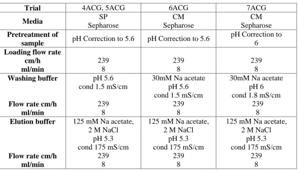
In the following tables are reported the operating conditions adopted in the batch experiments. The protocols are correlated to the results reported in table 1R, 2R, 3R respectively (see results, paragraph 3.1)

Table 1MM: Operating conditions of batch trials with SN/C

Trial 1B 2B 3B, 5B 4B, 6B Media CM Sepharose SP Sepharose CM Sepharose SP Sepharose Conditioning buffer 50 mM Na acetate, 500 mM NaCl pH 5.3 cond 46.8 mS/cm 50 mM Na acetate, 500 mM NaCl pH 5.3 cond 46.8 mS/cm 125 mM Na acetate, 500 mM NaCl pH 5.3 cond 46.8 mS/cm 125 mM Na acetate, 500 mM NaCl pH 5.3 cond 46.8 mS/cm Pretreatment of sample pH correction to 5.3 pH correction to 5,3 pH correction to 5.3 + dilution 1:2 with PW pH correction to 5.3 + dilution 1:2 with PW First and second Washing buffer 50 mM Na acetate, 500 mM NaCl pH 5.3 cond 46.8 mS/cm 50 mM Na acetate, 500 mM NaCl pH 5.3 cond 46.8 mS/cm 125 mM Na acetate, 500 mM NaCl pH 5.3 cond 46.8 mS/cm 125 mM Na acetate, 500 mM NaCl pH 5.3 cond 46.8 mS/cm Elution Buffer 50 mM Na acetate, 1 M NaCl pH 5,3 cond 85,8 mS/cm 50 mM Na acetate, 1 M NaCl pH 5,3 cond 85,8 mS/cm 125 mM Na acetate, 1 M NaCl pH 5,3 cond 96 mS/cm 125 mM Na acetate, 1 M NaCl pH 5,3 cond 96 mS/cm

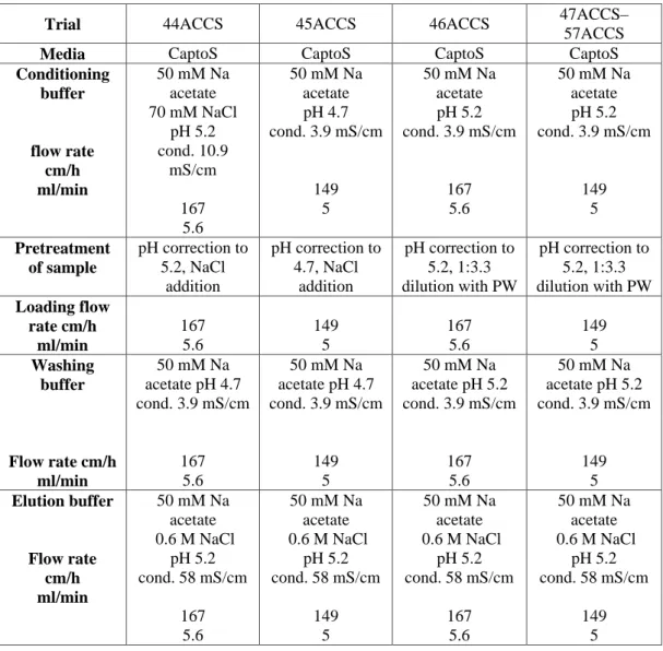
Table 2 MM: Operating conditions of batch trials with sample SN/I

Trial 7B, 11B 8B,12B Media CM Sepharose SP Sepharose Conditioning buffer 125 mM Na acetate, 500 mM NaCl pH 5.3 cond 46.8 mS/cm 125 mM Na acetate, 500 mM NaCl pH 5.3 cond 46.8 mS/cm Pretreatment of sample pH correction to 5.3 dilution 1:2 with PW pH correction to 5.3 dilution 1:2 with PW First washing buffer 125 mM Na acetate, 500 mM NaCl pH 5.3 cond 46.8 mS/cm 125 mM Na acetate, 500 mM NaCl pH 5.3 cond 46.8 mS/cm Eluate buffer 125 mM Na acetate, 1 M NaCl pH 5,3 cond 96 mS/cm 125 mM Na acetate, 1 M NaCl pH 5,3 cond 96 mS/cm