Chapter 3
The ANTARES experiment
The ANTARES experiment (Astronomy with a Neutrino Telescope and Abyss environmental RESearch) aims at the construction in the Mediterranean Sea of an array of about 1000 optical modules to form a high-energy (in the T eV ÷ P eV range) neutrino detector. In figure 3.2 the energy dependence of the effective area (see definition in chapter 2) for muon and neutrino detection is shown.
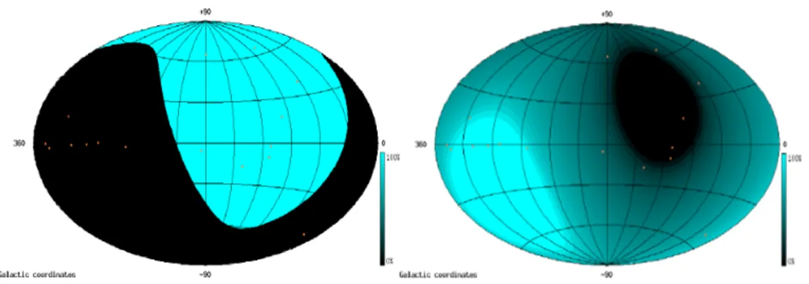
The experiment is somehow complementary to AMANDA. As can be seen in figure 3.1, the ANTARES detector covers the sky hemisphere opposite to the one visible from the South Pole (the total field of view is 3.5π sr, of which 0.6π sr overlap with AMANDA) and is therefore able to look at the galactic center 67% of the time.
Figure 3.1: Comparison between the field of view of the AMANDA (left) and ANTARES (right) experiment.
Furthermore, sea water is characterized by a longer scattering length than ice. 43
Hence a better angular resolution1can be achieved, allowing optimization for spe-cific physics targets and counterbalancing the drawback of the optical background (higher in sea than in ice). ANTARES will be characterized by a maximum angu-lar resolution better than 0.2oand a maximum energy resolution of about 10 GeV at 100 P eV . The energy dependence of these parameters is displayed in figure 3.3.
Figure 3.2: Effective area for neutrinos entering the Earth (left) and for ν-induced muons at the detector (right) as function of energy.
Figure 3.3: Left: Angular resolution for neutrinos and for muons as functions of energy.
Right: Muon reconstructed vs generated energy for Monte Carlo events. Black crosses
superimposed are a profile of the two-dimensional scatter plot.
The ANTARES telescope would extend its scientific programme within parti-cle physics and astrophysics.
The particle physics area, mainly concerning neutrino oscillations, has partly lost the importance it had when the ANTARES design started, in 1996, after the successful efforts of SNO [63], Kamland [64], SK and K2K [65] in validating the theory of neutrino oscillations and constraining the mixing angles and squared mass differences. Moreover, the energies involved in the study of atmospheric neutrino oscillations don’t well match the detection capabilities of ANTARES.
The detection of high energy neutrinos with unprecedented angular resolution is the most important aim of the ANTARES experiment mainly because of its astronomical implications. The principal mechanism for generating high energy neutrinos is through decay cascades originating in the interaction of high energy protons with matter or radiation. Hence the astrophysical sources of high energy neutrinos may also be the sources of the highest energy cosmic rays. Neutrino astronomy has already been discussed in the previous chapter.
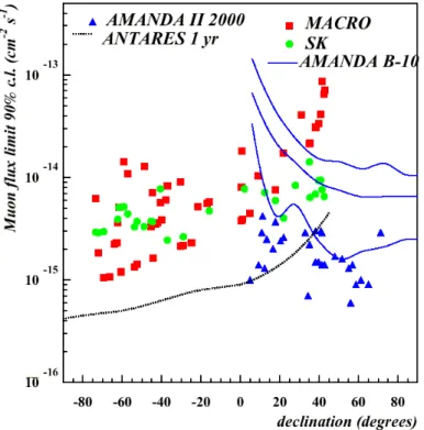
The ANTARES sensitivity to muon fluxes expected after one year of data tak-ing is shown in figure 3.4, compared with upper limits already set by measure-ments performed by other experimeasure-ments. The estimate of the expected fluxes from sources already known from gamma astronomy is very model dependent and it is not reported here.
Another ANTARES goal is a search, through the detection of neutrinos, for su-persymmetric dark matter relics in a region of the model parameter space which is interesting for cosmology and particle physics. Neutrino telescopes are not directly sensitive to WIMPs. However such particles could have been gravita-tionally captured in the cores of the Sun and the Earth or in the centre of the Galaxy. Their resulting high density would lead to annihilation reactions, which would then yield high-energy neutrinos through the decays of the gauge bosons and heavy particles produced. Compared to ongoing direct detection experiments, neutrino telescopes are generally more suitable for large WIMP masses, although resonances in the Earth’s capture cross-section are believed to strongly enhance the signal at certain lower masses, particularly around 56 GeV .
The two main noise components for the ANTARES experiment are an optical and a physical background. The first one is due to light sources different from the ˇCerenkov light from cosmic particles, like bioluminescence or ˇCerenkov light from radioactive decay products.
The behaviour of this background places constraints on the trigger logic and the electronics as well as on the mechanical layout of the optical modules. The measured rates are in fact very high, such as to constitute a hazard to the very
Figure 3.4: 90% confidence level upper limits on µ fluxes induced by neutrinos with
E−2 spectrum as function of source declination for SK, MACRO, AMANDA-B10 and AMANDA II. ANTARES sensitivity after 1 yr is also shown. It has not been possible to apply a correction due to different µ average energy thresholds (1.5 GeV in MACRO,
3 GeV in SK, 50 GeV in AMANDA and ANTARES). Nevertheless, the maximum of
the response curves of all detectors is at Eµ≈ 10 T eV , hence events contributing below 50 GeV should not make a large correction to these limits. [19]
functionality of the photomultiplier tubes (PMT) or to increase by large amounts data to be transferred to shore. A contribution of about 30 kHz comes from radioactive decays, in particular of the40K isotope. Bioluminescence present in sea water increases up to 50 ÷ 100 kHz the base noise rate and it also causes intense bursts up to tens of M Hz. Assuming the PMT nominal gain of 108, the charge per single photoelectron can be estimated as ≈ 10 pC: this means that the maximum anode current tolerated by the PMT (0.1 mA) is reached already at a rate of 10 M Hz.
The optical background is the main subject of this thesis and will be described in detail in chapter 4.
Besides40K and bioluminescence, the main light sources in deep sea originate from atmospheric muon ˇCerenkov light emission (about 300 γ/cm in the interest-ing wavelength range, between 300÷600 nm). Multiple downgointerest-ing muon events, which could constitute a background when misreconstructed as upgoing events, is suppressed by the detection depth. However, the vertical downgoing muon flux at a depth of 2400 m (10 ÷ 30 Hz depending on threshold energy and solid an-gle definition) is still about 106 times larger than the vertical upgoing muon flux from atmospheric neutrinos (see again figure 2.2). This is a formidable challenge for the detector. This second background component cannot be reduced with an appropriate on-line trigger, but it will need an ad-hoc filter based on the physical characteristics of the events.
3.1
Architecture
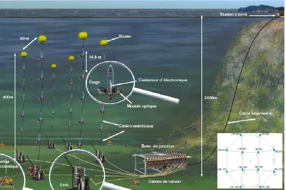
The detector consists of an array of 900 PMTs arranged in 12 vertical structures, called strings, anchored to the sea bed, spread over an area of about 0.05 km2 [23] and characterized by an active height of about 350 m. Figure 3.5 shows a schematic view of part of the detector array indicating its main components.
In conjunction with the detector string is foreseen the deployment of a dedi-cated line for monitoring environmental parameters (see section 3.1.2) and a fa-cility, the General Purpose Experimental Platform (GPEP), for oceanographic re-search which will be connected to the shore via the same junction box and electro-optical cable as the neutrino telescope lines.
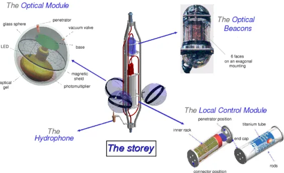
The basic sensitive unit of the detector is the optical module (OM), consisting of a PMT, a set of sensors for calibration purposes, and the associated electronics. The electronics includes a custom-built digital electronic circuit for PMT data ac-quisition, the high-voltage power supply for the PMTs and the network nodes for data transmission and slow control. The optical modules are housed in pressure-resistant glass spheres and are grouped together in clusters of three. Each of the 25 clusters of a single string is controlled by a separate electronic crate called local
control module (LCM). All the LCMs in a string are interconnected via an
electro-mechanical cable. This composite segment (OM cluster + LCM) is called storey, and a hydrophone and (eventually2) an optical beacons (OB) are also placed in it. The three OMs of a storey, the OBs, the hydrophone and the associated LCM are held by the optical module frame (OMF). The spacing between storeys is fixed to
2Since one OB is able to illuminate 8-10 storeys of each neighbour string, each detector line is
Figure 3.5: An artist view of the ANTARES detector. In the white square on the right, the horizontal layout of the 12 string is shown.
14.5 m and about 100 m divide the last storey from the sea bed, hence the total height of each line is about 450 m. As shown in the bottom-right corner of figure 3.5 the strings are arranged in an octagon with a minimum horizontal spacing of 60 m.
The optical modules in a storey are rigidly arranged in such a way that the axes of the PMTs point downwards, at an angle of 45o to the horizontal and with a horizontal angle of 120o between them. The angular acceptance of the optical modules is broader than ±70o(1.3π sr) with respect to the PMT axis. This means that the proposed arrangement detects light in the lower hemisphere with high efficiency, and also has some acceptance for muon directions above the horizontal. Moreover, in the hemisphere below the sea horizon, there is an overlap in angular acceptance between modules, allowing the possibility of an event trigger based on coincidences between nearby modules.
The relative positions and orientation of all storeys in the detector are given in real time by two independent positioning system.
and event reconstruction has to take into account their real position at each given moment. The precision of this spatial positioning should be better than the time uncertainty in light detection by the PMT (1 ns is equivalent to 22 cm of light travel path in water). The relative positioning of every OM of the detector is hence determined to an accuracy of 10 ÷ 20 cm (depending on the OM location and the current speed).
The first part of the positioning system is based on a set of tiltmeters and com-passes which measure local tilt angles and orientation of each cluster. The recon-struction of the line shape, as distorted by the water current flow, is obtained from a fit of measurements taken at different points along the lines: a maximum error of 1 m on the reconstructed shape is estimated, assuming a precision of 0.05o in tilt and of 0.3oin direction.
The second system, based on acoustic triangulation, is more precise but requires more complex and expensive electronics. The trasponder3placed at BSS of each string send an acoustic signal to a minimum of three transponders fixed to the sea bed, each of whom replies with its characteristic frequency which will detected by the hydrophones placed on each storey. A global fit of the measured acoustic paths gives the precise three-dimensional position of the rangemeters, provided that the positions of the transponders and the sound velocity in water are known4. The systems are complementary: a few points of the line can be measured acoustically and other points are obtained by line shape fitting.
In addition to the relative positioning of the OMs, the reconstruction of the muon tracks in the ANTARES detector depends on the relative timing of each phototube signal with respect to the others. A timing calibration with an accuracy of 0.5 ns must be achieved in order to avoid degradation of the 1 ns precision of the Cerenkov light arrival time measurements given by the photomultiplier.
A string is instrumented with several electronics containers. Each of these con-tainers constitutes a node of the data transmission network, receiving and trans-mitting data and slow-control commands. At every storey, a local control module (LCM) is located, and at the base of each string there is a string control module (SCM). Special containers house acoustics and calibration equipments. The con-trol modules support front-end electronics readout, sensor readout, slow-concon-trol parameters adjustment and trigger generation. Electronic containers also provide the distribution of power, master clock and reset signals to the front-end
electron-3Acoustic emitter-receiver.
4It is continuously monitored by a sound velocimeter with a precision of 5 cm/s and some
Conducivity Temperature Depth (CTD) devices record the variations of water temperature and salinity on which the speed of sound depends.
ics.
The individual SCMs are linked to a common junction box (JB) by electro-optical cables which are connected using a manned submarine. A standard deep sea telecommunication cable links the junction box with the shore station where the data are filtered and recorded.
The trigger logic off shore has been designed to be as simple and flexible as possible. Its main goal is to reduce the optical background contamination of physical events, without introducing a bias on event reconstruction. In the origi-nal intentions5: following a second-level trigger the full detector would have been read out.
The first-level trigger (L1) requires a coincidence between any two OMs in a sin-gle storey, which is highly likely in case of ˇCerenkov emission from an energetic muon, thanks to the typical wide emission cone in water and to the overlap be-tween PMTs angular acceptance in the same cluster.
A second-level trigger (L2) is based on combinations of first-level triggers. A more refined third-level trigger, imposing tighter time coincidences over larger numbers of optical modules, must be implemented using a farm of processors on shore: the readout rate is expected to be hundreds of kHz, but the corresponding data recording rate should be lower than 100 events per second.
The following sections of this chapter describe the various components of the detector in more detail.
3.1.1
The Detector Strings
Each of the 12 strings is mantained vertically by a buoy on the top and anchored on the sea bottom. Between the buoy and the anchor, the active part of the string comprises a series of elementary detector segments. These segments are stan-dardised and can thus be mass-produced and (if necessary) interchanged. String components are designed to resist corrosion by salt water and high pressure, to be watertight and to minimize light reflection. The planned minumum lifetime for each component is 10 years.
The configuration of the principal elements of each string is illustrated in fig-ure 3.6.
The bottom string socket (BSS) anchors the string to the sea bed, facilitates the electrical connection of the string to the network and permits the release and
5Recently it has been suggested to avoid in the initial phase of the experiment the use of any
Figure 3.6: Schematic view of a detector string. Only 3 of the 25 storeys are drawn here. Acronyms are defined in the text and itemized in appendix A.
subsequent retrieval of the string itself. Connection of the string to the network is performed by a submarine. In order to allow precise and simple string instal-lation, its construction has been optimized for handling on the deployment ship, resistance to shock, stability during descent. The BSS is instrumented for acoustic positioning.
The electro-mechanical cable (EMC) provides mechanical support for the string and enables the electrical interconnection of the detector string elements. It is capable of supporting tensile, torsion and bending stresses maintaining the string’s stability, and is flexible enough to facilitate string handling, deployment and retrieval. Electrical cables and optical fibres run through the EMC and enable power distribution and transmission of signals between two consecutive electronic containers (LCM or SCM).
A schematic view of the ANTARES storey and its main components is shown in figure 3.7.
The OMF is a titanium structure which supports the various elements placed within it, namely the optical modules, the LCM container a hydrophone6 and
Figure 3.7: The base elements of a storey.
possibly an optical beacon7 and supports the major traction forces that work on the string during deployment and recovery without transmitting them to the active elements.
Out of each set of five consecutive LCMs in every string, one is a master
LCM (MLCM) with a predominant role for trigger logic and clock distribution.
The MLCMs act as mediators between the SCM and the other four slave LCMs. Each group of five LCMs constitutes a sector: each string consists of five sectors. The Pisa group contributes to the ANTARES experiment with the integration and testing of a large part of the slave LCMs which will be necessary for the 0.1 km2 phase.
The top of the string consists of a buoy whose dimension and geometry are optimised to minimise hydrodynamic effects, such as dragging and vibration, by maintaining a suitable tension in the string. In addition, the buoyancy ensures a controlled resurfacing of the string during retrieval.
6For acoustic positioning. 7For the OM time calibration.
The optical module The optical module is the main sensitive element of the detector. The PMT and its associated electronics are housed in a 43 cm diameter, 15 mm thick, glass sphere, which can withstand pressures of up to 700 bars, produced by the Benthos Inc. Company. The sphere is made of two halves, one of which (the one opposite the PMT photocathode) is painted in black on its inner surface so as to give the OM some minimal directionality with respect to ˇCerenkov light detection without degrading its acceptance. The two halves have machined edges which form a seal when subjected to an external over-pressure. Attenuation of light at λ = 450 nm due to the sphere was measured to be less than 2%.
Silicone gel, covering the entire photocathode area, ensures both optical cou-pling and mechanical support of the PMT. Its refractive index (ngel = 1.40) does not exactly match that of the sphere (nglass = 1.48) but is higher than the refractive index of water (nwater = 1.35) in such a way as to minimize the amount of light reflected out of the OM. The attenuation of light caused by the gel is negligible with respect to the one due to the glass sphere.
A cage made of 1.1 mm thick high-permittivity alloy wire is used to shield the PMT from the Earth’s magnetic field and minimize the dependence of the detector response upon its angle to the magnetic North. The mesh size of the cage (6.8 cm) was optimized to reduce the non-uniformity of the PMT angular response to less than 5% while minimizing the fraction of light lost due to the shadow on the photocathode.
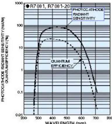
Figure 3.8: Hamamatsu measure-ments of Q.E. for PMT R7081.
Several PMTs of different diameters have been studied before coming to the final choice of the Hamamatsu R7081-20 PMT. It is a hemispherical tube made of borosilicate glass, 10 inches in diameter, with a bialkali photo-cathode and a 14-stage amplification system. The quantum efficiency for the specific com-bination of window and photocathode materi-als is shown if figure 3.8. The nominal gain of 108 is reached for a high voltage of about 2500 V . Its performances are summarised be-low in terms of a small number of critical pa-rameters, only a fraction of those which have been measured [27].
Electromagnetic interference in the OM in-duces less than 5 mV (rms) noise at the PMT
into account. A factor of 10 between the average pulse height for a single photo electron (SPE) and the pedestal is sufficient to ensure efficient discrimination of the signal. This corresponds to an effective working gain of the order of 5 · 107, but in view of ageing a maximum gain of at least 108 is required.
The effective photocathode area is defined as the detection area of the photocath-ode weighted by the collection efficiency. It was measured by scanning the entire photocathode surface with a collimated blue LED and a value of 440 cm2has been obtained.
The peak to valley ratio is computed from the observed charge spectrum of single photoelectrons with the high voltage adjusted to give 50 mV amplitude for SPE. It is measured to be 2 at the nominal gain of 108.
Due to small imperfections in the electron optics and the finite size of the pho-tocathode, the SPE transit time between the photocathode and the first dynode has a measurable width, usually referred to as the transit time spread (TTS). This defines the timing resolution of the PMT, which is required to be comparable to that from the overall positional accuracy (1.3 ns RMS) and the timing precision in the readout electronics (3 ns FWHM). The measurement of the TTS is performed over the whole photocathode area with the PMT operating at a gain of 108yelding 3.3 ns FWHM.
3.1.2
The Instrumentation Line
Knowledge of light and sound speed in water is essential for track reconstruction, while knowledge of deep sea currents will help to correlate effects visible in the data (detector position variation, optical background modulation, effect of sedi-mentation) with marine properties. The main ANTARES detector strings host a few instruments8providing the minimum amount of information needed for data analysis.
The Instrumentation Line (IL) is a totally dedicated tool for monitoring envi-ronmental properties relevant to the detector calibration and data analysis. running in parallel to the rest of the experiment.
In order to simplify the construction and the data collection the Instrumenta-tion Line uses the same mechanics developed for the other detector strings and the same read-out electronics and data transmission.
The basic instruments installed on the Instrumentation Line are:
Figure 3.9: The Mini IL, a prototype of the final Instru-mentation Line design.
• Acoustic Doppler Current Profiler (ADCP), to monitor the water current flow along the full height of the detector strings;
• Conductivity-Temperature-Depth (CTD) sen-sors, to monitor the temperature and salinity of the sea water at various depth;
• Sound Velocimeter, to monitor the sound ve-locity in sea water;
• Device to measure the light attenuation and absorption in sea water: a transmissiometer CSTAR of WetLabs;
• Seismometer.
It is also foreseen, at least at the beginning of the detector operation when only a few strings are de-ployed, that the Instrumentation Line will host the Laser Beacon and an Optical Beacon used for Optical Module time calibration.
The IL will be recovered (if needed) every one or two years to maintain instru-ments, to install new devices, and to monitor the behaviour of immersed material.
3.2
Offshore electronics and DAQ
The detector size and the distance between the detector and land do not allow to transmit analog signals and preclude a point-to-point connection between each OM and the shore station. Instead, an electro-optical cable from the shore station supplies electrical power to the detector array and permits data to flow in both directions using optical fibres. The electro-optical cable ends at the juction box to which the strings are connected. A star-topology network architecture is used, running from the string control module to the optical modules via the local control modules. A digital scheme has been devoloped for the necessary data multiplex-ing. This network is used to distribute power, collect data, broadcast slow control commands, distribute master clock signals, and form the trigger.
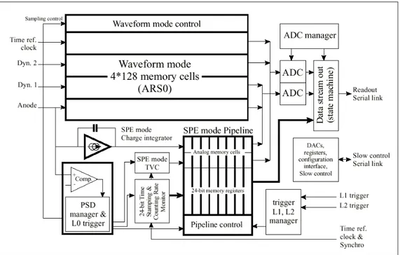
The OM electronics is constrainted by the limited space and power available. An Application Specific Integrated Circuit (ASIC) has been developed for the digital front end at the PMT output, tailored to the experiment needs. The cir-cuit is called Analogue Ring Sampler (ARS) and three9 of them are placed on the motherboard of each OM. Its block diagram is shown in figure 3.10. They
Figure 3.10: ARS1 block diagram
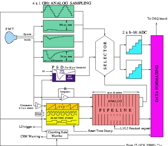
basically record all the pulse shapes either simple or more complex: the signal type is determined from a pulse shape discriminator (PSD) and processing is run in two different modes (WF and SPE). The PSD criterion is displayed in violet in the center of figure 3.11. The system allows to adjust the main parameters of the PSD, i.e. the large pulse threshold, the time over threshold and the time window for multiple pulses.
In figure 3.11 the main steps of data processing are shown. The chip samples the PMT signal10continuously at 1 GHz and holds the analogue information on 128 switched capacitors when a low-level threshold is crossed (L0 trigger). A
9Only two ARS per OM are used for data taking in a “token ring” (see below), while the third
one is used for triggering purpose only.
timebase 20 M Hz clock generated on shore is also sampled at 1 GHz on one channel, giving a relative timing of the signals to better than 1 ns. Only if the
Figure 3.11: General description of signal processing.
PSD finds that the PMT signal output is longer or higher than the reference value, the information is digitized by an external 8-bit ADC , i.e. the event is processed in the full wave form (WF) mode.
The same external 20 M Hz clock is used by the Time-to-Voltage Converter (TVC) as well as the Time Stamp (TS). The TVC provides an analogue value proportional to the time when the L0 threshold was crossed in between two con-secutive timebase clock cycles. Digitization by using 8-bit ADC provides time resolution of 0.2 ns.
The time stamp is obtained for each event by counting with 24-bit registers the 20 M Hz reference clock cycles.
A reset command sent through the clock stream is used to restart all the coun-ters of the array synchronously.
Almost 99% of the pulses are single photoelectrons, whose pulse shape is implicitly known from PMT calibration measurements. Hence, if the signal is within the PSD gauge, the processing returns only the charge and the arrival time at a threshold crossing, and the information is transmitted to shore along with the OM address. This SPE mode reduces the dead time due to the event processing and the data flow, because the related information needs only four words (8 bytes). For the remaining 1% of the pulses processed in the WF mode, the pulse shape is also transferred to shore for offline analysis and this implies the processing of a larger amount of data, namely 263 bytes per event.
The ARS chip has also two extra features independent from the signal pro-cessing: the counting rate monitor (CRM), which generates a CRM event after a predefined11 number of pulses, and the pulse generator for LED command12.
A pipeline memory is implemented to store the SPE information long enough to match the readout request (RoR) propagation and formation time, which is around 10 µs in the case of a RoR following a global L2 trigger. Two memories per optical module are used, in a token ring: the DAQ itself shares the data be-tween them sending the event to the first free memory. This will permit the chip to be used in case of counting rates exceeding 60 kHz and for a km-scale detector, where the trigger formation and propagation time may reach 30 µs.
3.2.1
Data formats
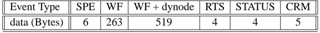
A summary of hit types and the corresponding data volumes can be found in table 3.1.
Event Type SPE WF WF + dynode RTS STATUS CRM
data (Bytes) 6 263 519 4 4 5
Table 3.1: Summary of the ARS hit data.
11This precount value is an adjustable number between 1 and 155.
12Single or 1024 pulses synchronised to the reference clock are delivered at a predefined rate or
SPE A single photo-electron hit is generated if an input trigger (L1 or L2)
co-incides with the (internal) L0 trigger of a hit. It contains the header, the integrated charge (1 Byte), the time stamp (3 Bytes), and the TVC.
WF A waveform hit is generated if the signal passes the PSD criteria. It contains
the SPE information and 128 samples of the anode signal. When both ARS chips are occupied by waveform hits, the data are reduced to those of a SPE hit. The PSD flag in the header is then set correspondingly.
WF+dynode A subset of waveform hits can contain waveform information from
dynode signals as well.
RTS Reset time stamp events are generated each time the internal clock register
is reset. This reset occurs when the ARS counter reaches its maximum or when an external RTS signal is applied. The header contains the last time stamp value before the reset.
STATUS Status events are generated by the ARS at power on or when slow
con-trol access starts or terminates. The ACQ/BUS flag in the header indicates the actual status. Status events contain the current time stamp value.
CRM Counting rate monitor events are generated by ARS each time the L0
pre-count is reached. It contains the header, time stamp and the time needed to reach the precount.
The data of each ARS are packed into frames and sent to shore by the process running on the LCM. A frame contains a header with information on the source, time stamp, data type, etc. When applicable, a list of hit items is included behind the header.
The frame header format13 that was read by the datafilter has the following format:
Raw ARS frame header (32 bytes):
FrameSize U32 Total length of frame in 4-byte words DataType U16 Data type code (SPE, WF etc.)
FrameTarget U16 On-shore farm PC handling this time slice FrameTime U64 Frame time stamp (units 50 ns)
FrameIndex U32 Frame number since start of run
NbItemsOrg U16 Number of L0 trigger happened in this data frame+ NbItems U16 Number of items sent in this data frame∗
LCM ID U16 Identifier of originating LCM
ARS ID U16 Identifier of originating ARS inside LCM RunNumber U32 Unique run number
+ From the FPGA, and not from the ARS. Implemented later.
* That is CRM items, for the PSL, rather than SPE items. The SPE format
has been used for sending CRM events, hence 6 Bytes instead of 5 Bytes are used with one Byte set to zero.
The setup of the run (ARS threshold and CRM precount, PMT voltages, etc) is stored in a database together with the run number and the frame-time dura-tion. The frame time duration is set through the slow control. During the entire life of the PSL in 2003 (see section 3.5.2), it was 219 LCM clock cycles14, i.e. 13107200 ns.
3.3
On shore data handling
Two main functions are implemented on shore: the data acquisition and the slow control for various aspects of detector operation.
The aim of the onshore data acquisition is to maintain an experiment status database using the slow control information, apply a filter of higher level with re-spect to offshore triggers (in order to reduce rates to a reasonable level for archiv-ing on tape) and verify the data integrity.
The main purpose of the slow control system is to initiate and verify the con-figuration of the detector (through in-situ calibrations and instrument settings), the initialisation of all processes and the changes between the possible states of the DAQ system.
The first step of the on-shore processing is event building. Here, time-stamped data from various parts of the detector are assembled into events. Most of the
triggers are caused by accidental coincidences and these may be filtered in off-line reconstruction. The event building will associate both digital data from the OMs and slow-control data in the same event. Fully built events will be used for feedback in controlling the detector, as well as for event display and data monitoring. A Unix-based event display has been developed (and tested using the prototype strings) for this purpose. An online monitoring system is also used to monitor the quality of the data and the stability of the detector. This reduces the time required to detect errors and speeds up the verification procedure after expert intervention(s).
PMT voltage, temperature and power-supply voltages are read from the OMs, while information on string attitude, water current speed, acoustic positioning in-formation and other control data are provided by dedicated instruments. Parame-ters to be adjusted during detector operation include the PMT voltage, thresholds involved in pulse detection and triggering, and various calibration systems. Slow-control data acquisition and execution of slow-control commands are car-ried out by the processor on the motherboard of the relevant electronics container (OM, LCM, SCM or specialized instrumentation containers).
3.4
Trigger logic and rates
A schematic drawing of the off-shore trigger logic is displayed in figure 3.13. Only a level zero trigger is still used for the readout of single hits.
The level zero trigger occurs when the output of a PMT crosses a threshold corresponding to 30% of a SPE amplitude. Two peculiar examples of L0 triggers depending on the time duration of an event are shown in figure 3.12. The L0 trigger signal has a minimum time duration of T wmin, adjustable between 10 ns and 70 ns, and the maximum pulse width is 4 times T wmin. Setting limits to the pulse width is needed in order to made coincidences between two OM in case of low amplitude pulses leading to very short Time Over Threshold (TOT) and to avoid any extra triggers in the falling tail of large amplitude pulses.
In order to deal with the high counting rate in the sea (see section 4.1), a level 1 trigger is built out of a tight time coincidence (20 ns) between two L0 triggers from the same storey.
A level 2 trigger can be formed by requiring multiple L1 triggers in a coinci-dence gate whose width is of the order of that needed for a track to pass through the entire detector (about 2 µs). The L2 trigger condition could be at least two L1 triggers on the same string (L2 1: string trigger) or at least three L1 anywhere in
Figure 3.12: L0 trigger timing examples
the detector (L2 2: array trigger).
When either the string trigger or the array trigger conditions is satisfied, a readout request is sent to the entire array. The readout request is received in each ARS, which starts the digitization of all the information within the maximum allowed muon crossing time. Internal delays specific to each OM compensate for the trigger formation and readout request propagation times. When an L1 trigger occurs in a storey, the two OMs involved are read out, even if they do not participate in the subsequent L2 trigger.
The L1 trigger logic will be installed in each LCM, in the ARS mother-board and in a specific trigger mothermother-board of each LCM which uses Field Pro-grammable Gate Array (FPGA) circuits. The L2 trigger logic must be linked to all the LCMs which may participate in the trigger, therefore the array trigger is installed in the junction box, while the string trigger will be installed at the bottom of each string (in the SCM) and then sent to the JB from which the readout request will originate.
The volume of data transmitted to shore depends on the trigger rate, the OM background and the proportion of WF events. Trigger rates and data flow due to random coincidences from background counting rates will be here estimated, in both cases of a readout request following either L0 or L1 trigger, assuming optimistic values of 75 kHz for the L0 trigger base rate and a contribution from burst events during 30% of the time.
During a bioluminescent burst, L1 triggers from affected storeys provide no discrimination against noise, because often all the OMs in the storey “see” the
Figure 3.13: Trigger logic. The avoidance, in the initial phase of the experiment, of global RoRs has been recently suggested: all data generating a L0 trigger would be sent to shore.
burst. These storeys are removed from the trigger logic in real time, but the OMs are still read out, though it will be hard to recover the signal from the noise when tracks are reconstructed. Let us assume that the L1 trigger is disabled for modules affected by bioluminescence events (threshold at 500 kHz). From a distribution of raw rates one can extrapolate that the dead time in the detector will be less than 10% and the effective burst fraction will be reduced to 20% (with an average rate reduced at 300 kHz).
The average number of possible random coincidences in a OM triplet is 2 · 3!
2!(3−2)! · R1 · R2 · τ . Assuming R1 = R2 = R3 = 75 kHz 70% of the time and R1 = R2 = R3 = 300 kHz 20% of the time, and using the L1 coincidence window τ = 20 ns, the L1 trigger rate will be: 6 · (112.5 · 0.7 + 1800 · 0.2) Hz ≈ 2.6 kHz per storey, or 12 · 25 · 2.6 kHz ≈ 800 kHz for the entire detector.
Accidental overlap of consecutive signals in the 50 ns integration gate pro-duces wide pulses detected as WF events 1% of the times at the base rate and 4%
of the times in burst regime, which on average correspond respectively to 68.6 bits and 130.2 bits per hit. Under these assumptions, the data flow rate for a readout15 of the entire detector (900 OMs) following a L1 trigger is 6 · (112.5 · 0.7 · 68.6 + 1800 · 0.2 · 130.2) · 3 bits/s ≈ 940 Kbits/s per storey or ≈ 2 Gbits/s for the entire detector. The use of one of the type of L2 triggers described above will further reduce this number.
In a future situation of single L0 triggers readout, assuming the same 500 kHz cutoff for bioluminescence, the average OM trigger rate would be (75 ∗ 0.7 + 300 ∗ 0.2) kHz ≈ 100 kHz, the average OM data flow rate would be (75 ∗ 0.7 ∗ 68.6 + 300 ∗ 0.2 ∗ 130.2) Kbits/s ≈ 11 Mbits/s, and the average data flow rate for the entire detector would reach 10 Gbits/s.
3.5
Status of the experiment
Since its very beginning ANTARES has followed an R&D programme focused on three major milestones:
• The construction and deployment of test lines dedicated to measuring en-vironmental parameters such as optical background, biofouling and water transparency.
• The development of prototype strings to acquire the necessary practical ex-pertise in the deployment and operation of an undersea detector up to the kilometer scale (see chapter 2).
• The development of software tools to explore the physics capabilities of the detector (see section B).
This R&D phase has demonstrated that the deployment and physics operation of such a detector is feasible. As a consequence, the construction of the detector is starting.
3.5.1
Site environmental parameters
The Mediterranean Sea represents an environment for a neutrino telescope that is quite different from those of the operating arrays at Lake Baikal (a freshwater lake which freezes in winter) and the South Pole.
Therefore, in order to ensure the success of the deployment of a large scale detector in such an uncontrollable environment, an extensive programme of site evaluation and prototype testing has been necessary. A continuous environment monitoring will be done during the entire detector operation, thanks to a dedicated instrumented line deployed in conjunction with the 12 detector strings (see section 3.1.2). The detector will be deployed at a site near Toulon, at 42o500 Northern latitude and 6o100 Eastern longitude, at a depth of 2400 m under the sea level. The final choice of the site, illustrated in figure 3.14 satisfies the requirements
Figure 3.14: The ANTARES site, in the South cost of France.
on water transparency, optical background, fouling of optical surfaces, strength of the deep sea currents, meteorological conditions and depth. It also presents several advantages for the geographical position which allows an efficient on-shore support and is characterized by a large availability of infrastructure and pier.
Water optical properties The water transparency affects the muon detection efficiency, while the amount of scattered light determines the detector angular resolution. The optical properties also place strong constraints on the detector
geometry, because light attenuation limits the maximum spacing between opti-cal modules that allow a good reconstruction of tracks with no information loss. Measurements and analysis performed in the ANTARES site [21, 22] give an ab-sorption length in the range 25 ÷ 55 m and an effective scattering length in the range 120 ÷ 300 m from UV to blue light (370 ÷ 470 nm).
Fouling The surfaces of optical modules exposed to sea water are affected by the combination of two fouling processes. The first one is the growth of living organisms, mostly bacteria, on the entire outer surface of the glass sphere. The second process is the fall of sediments, mainly originating from continental river beds, on upward-looking surfaces. The bacterial growth is almost transparent, but sediments adhere to the surface and make it gradually opaque. As shown in figure 3.15, measurements have demonstrated that fouling is significantly reduced for polar angles larger than 50 degrees with respect to the zenith. At the equator (θ = 90oin figure 3.15), the fouling induces a transmission loss which saturates to 1.5% after eight months of immersion. This is an upper limit on the loss expected on the actual detector, where optical module axes will be oriented at a polar angle of 135 degrees with respect to the zenith [34].
Figure 3.15: Light transmission as a function of time and polar angle.
Sea conditions Suitable sea conditions are required to perform deployment and recovery operations. These conditions depend both on the nature of the operations and on the characteristics of the ship. The favorable sea conditions specified for operations with the boat Castor16, for example, are a wave height lower than 1.5 m and a wind speed lower than 25 knots17. The analysis of data from a number of sources leads to the conclusion that periods of three consecutive days with these
16Belonging to the SERRA-MARINE company. 17Force 5 on the Beaufort scale.
specific conditions occur less than five times per month between October and April, and more than five times per month from May to September.
The strength and direction of undersea currents has been taken into account in the mechanical design of the detector. The strings well tolerate the maximum current speed presently observed, namely 19 cm/s (see section 4.1.3).
A visual and bathymetric survey of the sea floor was also performed in the potential sites. It checked the absence of topographical anomalies, such as steps or rocks, which could obstacle the string deployment and anchoring and it also made sure that the floor substrate will be a satisfactory support for the detector.
3.5.2
Prototype lines deployed in 2003
In 2002/2003, the ANTARES collaboration has deployed at the ANTARES site a prototype line made of one single sector (PSL, Prototype Sector Line: deployed in December 2002) and a first version of the instrumentation line (MIL, Mini Instru-mentation Line: deployed in February 2003) which have allowed the verification of the “final” design, in the final environment, using prototype electronics boards. They were intended to identify any problems as early as possible, in order to cor-rect them before the production of the full 0.1 km2 detector.
The sea deployment has permitted testing of many aspects of the design which would have been impossible to study in on-shore tests: the deployment/recuperation procedure itself, the power distribution via the sea electrode, the line movement, the acoustic and absolute positioning, the medium term corrosion effects, the eval-uation of system reliability, to name but a handful.
Unfortunately, testing trigger rates and data volumes in final conditions, as well as in situ time calibration with OM flashers and optical beacons (with real scat-tering and absorption effects), had not been possible because of the lack of the global 20 M Hz clock from shore, due to a problem with the optic fiber which was intended to transmit the clock signal generated on shore.
The sector line consists of a single sector of 5 storeys, with the associated SCM/SPM and BSS, and a minimal DAQ system at the on-shore station. The lowest storey is at the nominal position, 100 m from the sea bed, and the spacing between storeys is the old standard 12 m.
The MIL was equipped with 2 storeys separated by 100 m and a BSS. The devices in the upper storey were the ADCP and the sound velocimeter, while in the bottom storey the CT probe and the transmissiometer were located. The seismometer was positioned 50 m away from the MIL anchor.
Figure 3.16: The layout of the two prototype strings as appeared after March 2003. PSL shown on the left, MIL on the right.
Both the MIL and the PSL were connected to the Junction Box in March 2003, and it was planned that they would be operating in conjunction. However, a water leakage due to a faulty washer of the MIL forced the recovering of the line for debug almost immediately (April 2003), while the PSL continued its operations until the first weeks of July.
Furthermore both lines have been affected by several problems.
The main issues on the MIL have been the failure of clock distribution for trig-gering the acoustic positioning system (because of a break of the optical fibre), and the water leak on the MLCM which damaged MLCM and LCM electronics (the latter because of migration of water through the EMC). The acquisition of the environmental parameters (seismic activity, light absorption, sea currents, sound velocity, conductivity, pressure, temperatures) was not impeded by the clock prob-lem, but data were collected for 3 days only due to the flood of the MLCM. In the PSL, the early failure of some capacitors on the PMT basis, a problem with
a DC/DC converter on the same location and some booting problem caused the malfunctioning of all three OMs of LCM 2, while the LCM 3 stopped working because of a water leak. Moreover the clock did not propagate from the SCM to the LCM clock-boards, because the high pressure and tension endured by the de-manded fiber harmed the signal transmission. Without the clock, the ARSs cannot be enabled, therefore neither SPE18nor WF events could be acquired, but they did transmit some data even though not enabled: the CRM events. These can be used to measure the singles rates as functions of time, HV and ARS threshold values. In absence of the global clock, the LCM clocks have local 20 M Hz oscillators, which are not synchronised19, though.
Figure 3.17: MILOM layout, as agreed upon in March 2004.
For the next future, between the end of this year and the beginning of 2005, the deployment of two “new” test strings is scheduled: the MILOM, a new 3-storeys version of the MIL with optical modules and the old devices but new electronics, and again the (repaired) PSL line, with 4 storeys only (the broken LCM 2 will not be replaced) and using a new reinforced EM cable.
The main objectives of MILOM and PSL2 are the validation of the new EM Cable in real con-ditions, the test and validation of the new elec-tronics, long term monitoring of environmental parameters and their correlations, procedure de-velopments and checks for in situ calibration, and all those tests which were not possible with the MIL and PSL because of the failures mentioned above.
The deployment of the first of the 12 final strings will take place only a few months later and the whole detector will be operational within the following two years.
18For more details on data formats, see section 3.2 and section 3.2.1.
19If they had been synchronized a time resolution ≈ 25/√12 ns would have been gained on