5 - GROUNDWATER FLOW MODEL FOR THE COASTAL
PLAIN AQUIFER SYSTEM
The simulation of groundwater flow systems using computer models is standard practice in field of hydrology (REILLY & HARBAUGH, 2004). Models are used
for a variety of purpose: education, hydrologic investigation, water management and legal determination of responsibility.
A numeric model is a simplified representation and a mathematical approximation of a real situation. Jacob Bear, prominent theoretical about groundwater flow define a mathematical model of a site as: a selected simplified version of real system and phenomena that take place within it, which approximately simulates the system’s excitation-response relations that are of interest (BEAR, 1972). In Hydrology this abstract system is constructed to reproduce
in a simplified way a complex hydrogeological system, usually in order to verify the operation and predict the evolution in time.
It is important to distinguish among three term used in modeling process: conceptual model, computer model program and model. A conceptual model is the hydrologist’s concept of groundwater system. A computer model program is a computer program that solves groundwater equation. Finally, a model is the application of a computer model program to simulate a specific system. A model incorporates the model program and all the input data required to represent the real system and defined in the conceptual model. A mathematical model consists of differential equations describing in hydrogeology the flow and solutes transport. These equations contain the hydraulic properties of the aquifer (K, T, S, effective porosity) and are therefore able to reproduce the physical processes active in the aquifer system, once defined the initial conditions and boundary conditions. The calculation technique consists in the replacement of the mathematical equations with simple algebraic equations, repeated for a discrete number of points in the spatial and temporal domain. In other words, the unknown variables of the equations are related to a discrete system of nodes. The discretization methods more commonly used are Finite Difference Method (FDM) and Finite Element Method (FEM). The model program used in this study is Modflow (HARBAUGH et al.,
2000) and it is a FDM. For more details, please refer to the literature (BEAR, 1972;
1979; 1987; ANDERSON & WOESSNER, 1992; MCDONALD & HARBAUGH, 1988; HARBAUGH
et al., 2000; REILLY & HARBAUGH, 2004, FEINSTEIN, 2010, RUMBAUGH & RUMBAUGH,
The phases for the construction of a mathematical model, all extremely important for a correct numerical reproduction of the aquifer system, are the following:
1. Defining the objective of the study 2. Development of the conceptual model
3. Development of mathematical model based on conceptual model
The computer model code used in this study is MODFLOW (Harbaugh et al., 2000), the U.S. Geological Survey modular finite-difference flow model. Numerous software are commercially available that contain a graphical interface that allow to set the model more or less rapidly on the computer and then move to the stage of calculation with the chosen code, in this study GROUNDWATER VISTAS 6 which provides a graphical interface for MODFLOW was used.
The procedure for defining the mathematical model with the help of the graphical interface provides a series of operations described in detail in the following chapters.
5.1 DISCRETIZATION AND REPRESENTATION OF THE
HYDROGEOLOGIC FRAMEWORK
A fundamental aspect of numerical model is the representation of real system by discrete volume of material. In the FDM the volumes are called cells. The size of the cells determines the extent to which hydraulic properties and stress can vary in the modeled region. The hydraulic properties and stress are specified for each cell, so more cell are present in the model major is the ability to vary the proprieties and stress. As regard the vertical discretization two approaches are used to represent the hydrogeologic framework in the model: uniform model layer and deformed model layer. In evaluating a groundwater flow simulation the proper and sufficient discretization is not straightforward to determine. Enough detail is required to represent the hydraulic properties, stress and complexity of the flow field; yet, the cost will be less if the model is kept as simple as possible so that data entry, computer resources and analysis of model output are as minimal as possible. Thus, the determination of the proper discretization is always a compromise (REILLY &
HARBAUGH, 2004).
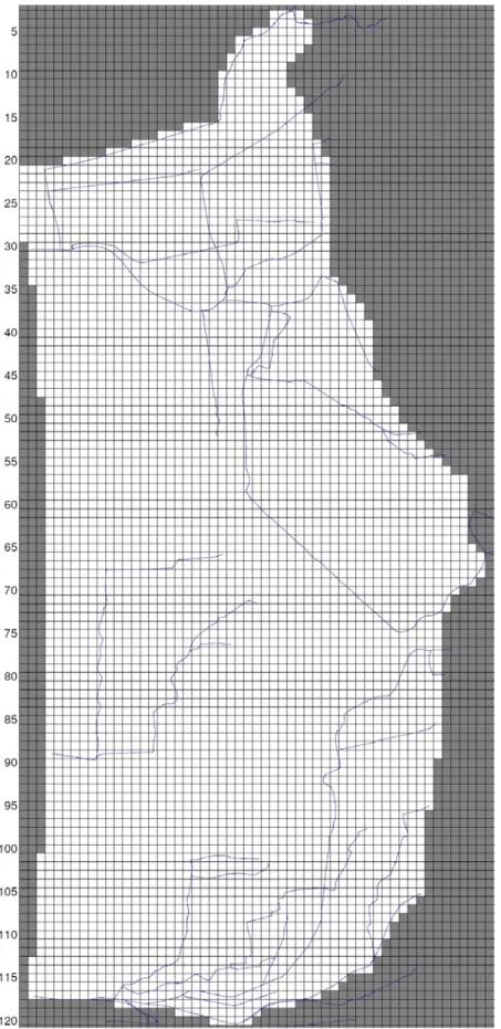
The area of interest is about 10 km long and has a transverse extent average of 4 km. The total area is about 52 kmq. The discretization of the model consists of 121 rows, 55 column (figure 5.1) and 4 layers for a total of 26620 cells (which 17616 cells are active). The spacing of the cell is 100mx100m, whereas the bottom and the top of the layer is been imported following the hydrostructural model discussed in the chapter 4.1.
Figure 5.1 – Discretization of the area with cells spacing 100x100m. The cells grey are no-flow cell.
5.2 SPECIFYING PROPERTIES OF CELLS
An important aspect to represent the hydrogeological frame work is the choose of the hydraulic properties assigned to the cells. Given the uncertainty of knowledge of the distribution of these properties groups of cells a uniform value rather than attempting to define an individual value for each cell are usually given. The assignment of hydraulic properties of the system means the reproduction of the main aquifer, aquitard and aquiclude in terms of geometrical and hydrodynamic parameters (Hydraulic Conductivity, Transmissivity, Specific Storage, Specific Yeald, porosity).
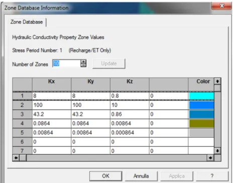
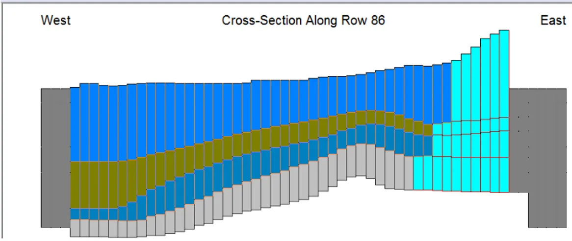
The assignment of the hydrodynamic characteristics is performed on the basis of data from pumping tests found in literature and on the pumping test conducted during this study and described in detail in chapter 4.1. In addition to the definition of hydraulic parameters are been taken into account the granulometric composition defined for each layer of the hydrostructural reconstruction, described in detail in chapter 4.1. In figure 5.2 are reported the hydraulic conductivity class selected and used for the assignment to the cell in the model, whereas in figure 5.3 is reported a cross section along row 86 where it is possible to observe the different vertical discretization for each layer.
Figure 5.3 – An example of hydraulic conductivity zone assigned to cross section along row 86. For the colours see figure 5.2.
5.3 REPRESENTATION OF BOUNDARY CONDITIONS
Boundary condition are a key component of the conceptualization of a groundwater system. The topic of boundary condition in the simulation of groundwater flow was discussed in FRANKE at al. (1987) and REILLY (2001). As
noted computer simulation of groundwater flow systems numerically evaluate the mathematical equation governing the flow. This equation is a second-order partial differential equation with head as the dependent variable. To determine an unique solution it is necessary to specify boundary condition around the flow domain for head (the dependent variable) or its derivates. So a requirement for the solution of the mathematical equation is that boundary conditions must be prescribed over the boundary of the domain. Boundary conditions also represent any flow or head that constraints within the flow domain, like as recharge, river interaction and pumping by well.
The choice of boundary condition, to be used for a specific hydrogeological conditions, is one of the most delicate and important phase in a numerical modelling because they influence the numerical solution and define how much water enters and leaves the domain of the model.
Three type of boundary condition are commonly used and in the following briefly describe:
I. Specific head or Direchlet (I type): specified head boundary cells represent a constant head limit. They correspond to hydrogeological discontinuities that under particular hydrodynamic (natural or artificial) conditions allow to maintain a constant water level in both incoming and outgoing with respect with the domain. The flow that enters or leaves the system is in proportion to the difference between the head specified in the boundary and the head of the adjacent cells.
II. Specific flux or Neumann (II type): specified flux boundary cells are represented using no-flow (or inactive), wells, or recharge. They correspond to particular hydrogeological discontinuities that under particular hydrodynamic (natural or artificial) conditions allow the passage of selected flow incoming and outgoing with respect with the domain.
III. mixed or Cauchy (III type): mixed-type boundary conditions are called rivers, drains, general-head boundaries, streams, or evapotranspiration. They correspond to a mixed of the other ones.
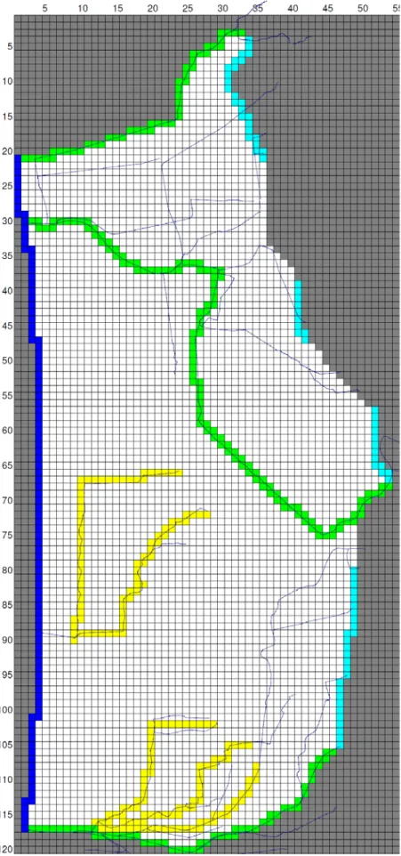
The boundary conditions used in this model are been selected on the basis of the conceptual model, in particular have been used the following types of boundary condition (figure 5.4):
- Specific head or Direchlet (I type) for the coastal line (head=0).
- No Flux (II type) along the NE boundary for the cells that represent the contact between the incoherent deposits of the plain with the impermeable no-carbonatic rocks of the foothill area, that should not contribute appreciably to the recharging of the system.
- General Head Boundary (GHB) conditions (III type) along the NE boundary of the domain for the cell that represent the contact between the incoherent deposits of the plain with the permeable carbonatic rocks of the foothill strip. - General Head Boundary (GHB) conditions (III type) along the NE boundary for the alluvial fan of the Versilia River and T. Montignoso alluvial fan in the northern part of the area.
- River (III type) for the Versilia River in the central part of the area and T. Canalmagro stream at the boundary north and T. Baccatoio stream at boundary south.
- Drain (III type) for the “low level water channel” discussed in the chapter 2.2
Even recharge for rainwater infiltration and pumping from wells and dewatering, following described, can be considered as boundary conditions being imposed flow limits (II type).
Recharge
For the quantification of the recharge as input to the system the average annual rainfall and average annual temperatures were used. These value are needed to assess the real evapotranspiration (Er) and effective infiltration (P = Ie-Er * CIP, where CIP is potential infiltration coefficient). The value of temperature and rainfall were collected from “Ufficio Idrografico e Mareografico della Provincia di Pisa” and from the website of ARSIA (www.arsia.toscana.it). In particular, the station located near Massa city was considered the reference station because has thermometric and pluviometric data available for a greater time range: 1926 to 2002 for precipitation, and from 1942 to 1999 for the temperatures. This station doesn’t located inside the area of study, but in the area just to the north. By a comparison of the data of Massa station with data belonging to stations located in the area of interest, the Massa station seem to be hydrometeorologically representative of the entire area.
Taking into account the data sets available, a representative mean hydrological of 30 years is considered, and in particular from 1980 to 2010. To fill the missing years for the temperature data (from 2000 to 2010) and precipitation (from 2003 to 2010) was carried out a process of comparison with stations in neighbouring areas for which these data were available during the same period. In particular, both the rainfall and temperature data of Massa station were compared with data from the station of Lido di Camaiore (data available from 1990 to 2010) for the years in common (from 1990 to 2002 for precipitation and from 1990 to 1999 for temperature).
As regards the rainfall a linear correlation was calculated and defined by the following relationship:
y=0.7902x + 412 (R2=0.9022)
Based on this equation average annual rainfall for the lacking year of Massa station are been recalculated. In this way a mean annual value of precipitation of 1181 mm is calculated, refers to average hydrological year of 30 years (1980-2010).
As regards the temperature was performed the same procedure of comparison for the years in common between the Massa station and Lido di Camaiore obtaining the correlation equation:
y=0.8386x+3.6265 (R2=0.9097)
Based on this equation the mean annual temperatures for the lacking year of Massa station were recalculated. In this way a mean annual value of temperature of 16.04°C is calculated, refers to average hydrological year of 30 years (1980-2010).
Obtained the value of annual average precipitation and temperature the real evapotranspiration was calculated according to TURC method (1954), equal to 733
mm per year always refer to the same average hydrological year of 30 years, obtaining a value of effective precipitation (P-Er) equal to 448 mm.
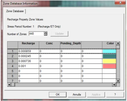
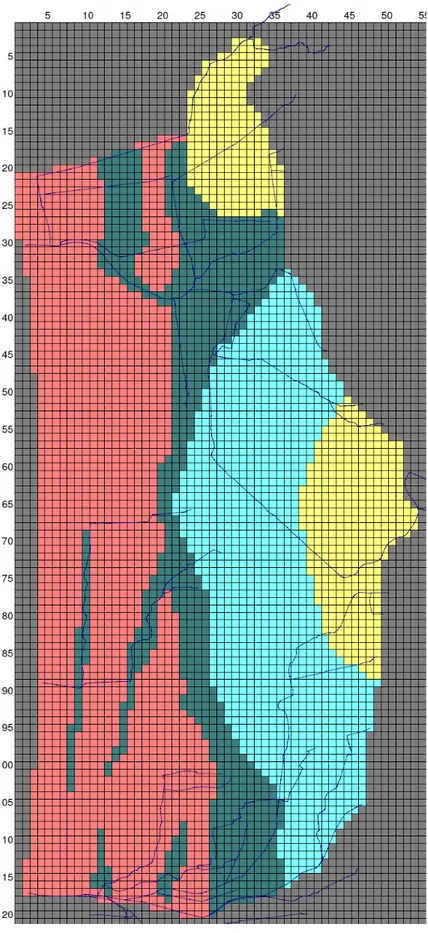
The recharge, as the water that inflow below the soil in to aquifer, is calculated multiply the effective precipitation by a Cip coefficient (Effective Infiltration Coefficient) depending of the outcropping deposits, the residential/industrial areas and the morphology. In particular for the model are been individuated 4 zone with different recharge reported in figure 5.5 (the value are reported in m/d). Instead in figure 5.6 is reported the spatial distribution of the recharge.
Figure 5.5 – Recharge zone expressed in m/day.
Pumping Well
In the area of study beyond 3000 well belonging to domestic use, drinking water, industrial use, agricultural use and other uses (data from BDSRI database) are present. Unfortunately, only for the drinking water wells the flowrate data is available, provided by Gaia srl, whereas for the other uses (domestic, agricultural, industrial and other) aren’t always available. To estimate the flowrate value and the time of pumping the few data available and some literature works were considered (TESSITORE, 2002; PRANZINI, 2004). So the average mean withdrawal and the
activity period were evaluated as:
Æ industrial well: in the BDSRI the flowrate reported is 3 l/s and the time of activity is been evacuate in 8 hours/day for 300 days in a year.
Æ domestic well: it is considered an average withdrawal of 1.5 m3/day for 150 days in a year.
Æ drinking water: the withdrawal for the well located in Lucca province is been provided by Gaia srl, whereas for those in Massa province is been estimated by literature data.
Æ agricultural wells: for these well it is considered a withdrawal of 3 l/s for 6 hours/day for 90 days in a year.
Æ other use well, mainly seasonal activities, it is considered a withdrawal of 3 m3/day for 150 days in a year.
Figure 5.6 – Recharge zone assigned at the first layer of the model. For the colours see figure 5.5.
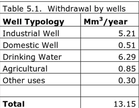
In the table 5.1 are reported the average annual value of withdrawal as regards the different uses for a total of 13.15 Mm3/annui.
Table 5.1. Withdrawal by wells Well Typology Mm3/year
Industrial Well 5.21 Domestic Well 0.51 Drinking Water 6.29 Agricultural 0.85 Other uses 0.30 Total 13.15
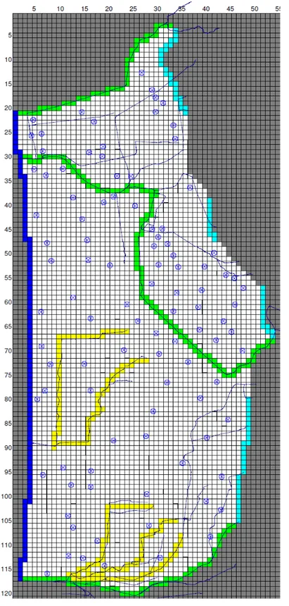
The pumping rate was set in the numeric model with point that represent a group of wells belonging to the same use and located in the same area for a total of 96 points (insert as “analytical well” in the software) (figure 5.7). The numerical model of this study is in steady state, so the flowrate determined are been distributed on 365 days.
Dewatering pumping
Vast areas of the plain are morphologically depressed and crossed by a network of shallow channels canals and drainages. Among these there are channels know as “high water” distinctly separated from the “low water”. The low level water channels, as described in the chapter 2.2, are used to drain the runoff from the mountains and the meteoric water. This is controlled by dewatering plants that collect the water towards channels of the high water and let them flow finally into the sea. The pumping rate was collected by literature study (TESSITORE, 2002)
where the data provided by Consorzio di Bonifica Versilia-Massaciuccoli are available. The dewater pumping are located in the depressed southern part near the T.Baccatoio stream and in the northern part, some near ex-Lago di Porta and some near the mouth of Versilia River. The withdrawal estimated on literature data is about 3 Mm3/y for the area of interest. The dewatering pumping are been imported
5.4 RESULT AND DISCUSSION
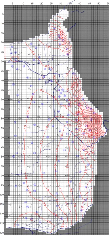
All data and value described above were used to create the numerical model of the aquifer system of the Versilia plain. In the figure 5.8 is reported the water table map calculated with the numerical model in steady state condition with the velocity vector and pumping well. In the map the isoline interval is 0.5 m for a best visualization in the coastal strip.
The calibration of the model was performed with the method “trial and error adjustment” as regards mainly the hydraulic conductivity and the pumping well that are the parameter more uncertain. The value obtained are compatible with literature data and the conceptual model delineated in the chapter 4.
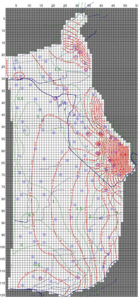
The comparison of water level map with a “mean piezometric map”, specifically created for this purpose using the mean value between the campaign of low and high condition level in 2009 (discussed in the chapter 4.1), shows that the general geometry of the isopiezometric line is the same (figure 5.9).
As regards the difference between the calculated value by the model and the average piezometric really measured in this project, some target with the “reference value” (43 points) consisting in the average between the high and low level condition measuring in the 2009 campaigns were imported. In the figure 5.10 these target are reported with the post residual of calibration. The value are very low, ranging from 1.18 to -1.02. The blue value indicate that the target value is major than the value estimated in this point, so the model underestimate, whereas a red value indicate the target value is minor than the target value, so the model overestimate.
Figure 5.9 – Water table map calculated with the numerical model (red lines) and piezometric map performed in this study (green lines).
0.5 0 -0.5 1 1.5 2 4 1 0.5 1 1.5
Figure 5.10 – Water table map calculated with the numerical model (red lines), target point and post residual values.
In figure 5.11 the statistic of the target are reported, where it is possible to observe that the value of Residual Mean, Residual Standard Deviation and Absolute Residual Mean are respectively 0.04, 0.62 and 0.53. In addition the Residual Sum of Square is 16.5.
Figure 5.11 – Target statistic
Finally as regard the target value in figure 5.12 the graph observed value versus model value is reported. The data are located along the line that represent the ratio between these value equal to 1.
Figure 5.12 – Observed value vs model value
In conclusion is reported the mass balance relating to the entire area of interest (figure 5.13 a e b) where it is possible to see that the major input at the
system is due to local precipitation for over 33000 m3/day, whereas the major
output from the system is obviously the pumping well with over 35000 m3/day. The
rivers feed the aquifer system with over 10000 m3/day, whereas they drain the
system with 231 m3/day.
Figure 5.13a – Mass balance relating to the entire area of interest.
In particular as regards the F. Versilia river the area was divided in three zone (figure 5.14) to highlight the input and the output from the system. The mass balance regarding the zone 1 (figure 5.14a) indicates that in this area the river feeds the aquifer with over 2000 m3/day. The mass balance regarding the zone 2
(figure 5.14b) shows that the river in this area isn’t in connection with the aquifer system with only 29 m3/day of input at the system. Finally the mass balance
regarding the zone 3 shows that in this area the Versilia river feeds the aquifer with over 2300 m3/day and it drains with about 230 m3/day. These values confirm the
conceptual model delineated in the chapter 4.
Figure 5.14 – Zone individuated to study the relationship between F.Versilia river and groundwater.
Zone 3
Zone 2
Figure 5.14a – Mass balance of the zone 1.