Chapter 3

9

Chapter 3

TEST VEHICLE AND LATERAL FORCE

MEASUREMENTS

3.1. Research vehicle and test equipment

3.1.1. Introduction

In this section the test vehicle and all the sensors used for the measurements are presented. These are part of the sensor equipment used by the Volkswagen Electronic Stability Programme (ESP), which prevents the vehicle from skidding by selective intervening in the brake and engine management system [8], [9]. Only the longitudinal and lateral speed sensor is mounted on purpose on the vehicle, and for this reason the installation requires the knowledge of the vehicle’s Centre of Gravity (COG).

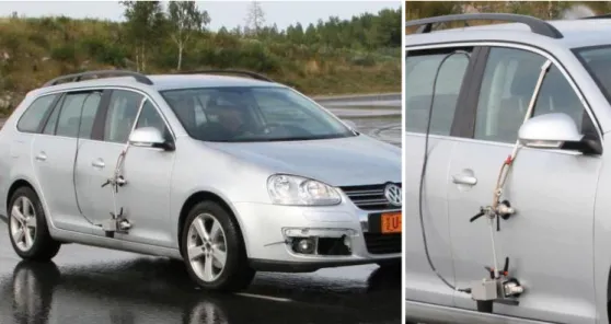
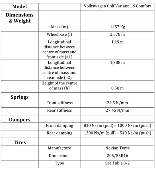
The test vehicle was a Volkswagen Golf V Variant 1.9 TDI (Figure 3-1) whose technical specifications are briefly presented (Table 3-1). The spring stiffness and shock absorber damping were obtained by previous measurements [10].

10

Model Volkswagen Golf Variant 1.9 Comfort

Dimensions & Weight Mass (m) 1457 Kg Wheelbase (l) 2,578 m Longitudinal distance between centre of mass and

front axle (a1)

1,19 m

Longitudinal distance between centre of mass and

rear axle (a2)

1,388 m

Height of the centre

of mass (h) 0,58 m

Springs

Front stiffness 24,5 N/mm Rear stiffness 27,45 N/mm

Dampers

Front damping 810 Ns/m (pull) – 1000 Ns/m (push) Rear damping 1300 Ns/m (pull) – 540 Ns/m (push)

Tires

Manufacture Nokian Tyres Dimensions 205/55R16

Type See Table 3-2

Table 3-1 – Volkswagen Golf technical specification

3.1.2. Steering angle sensor

The steering angle sensor is located on the steering column between steering column switch and steering wheel. It sends the steering angle signals to an electronic steering control unit via CAN bus, and those signals are here processed. It is shown in the Figure 3-2:

11

Figure 3-2 – Steering angle sensor [9]

The basic components of this sensor are:

a code plate that consists of two rings, an outer absolute ring and an inner increment ring;

photoelectric beam pairs, respectively with a light source and a optical sensor.

The increment ring is separated into 5 segments, each of 72° increments, and is read by a photoelectric beam pair, as shown in Figure 3-3. Within each segment the ring is split. The gap of the split is equal within the segments but different between the segments. This generates the code for the segments.

12

The absolute ring determines the angle. It is read by 6 photoelectric beam pairs. The steering angle sensor can detect a steering angle of up to 1044°. It accumulates the degrees after each turn of the steering wheel. In this way, it can detect that a full steering circle is complete when the 360° mark is exceeded.

The angle measurement is obtained by means of the photoelectric beam principle (showed in Figure 3-4), which is briefly summarized:

Figure 3-4 – Generation of signal voltage [9]

when light passes through a gap located in the outer (or inner) ring, this is detected by the optical sensor and generates a signal voltage. When light is covered, signal voltage is interrupted;

with the rotation of the ring a signal sequence is thereby generated;

this happens for each pair of photoelectric beam, and their signals are all processed by the steering control unit; by comparing the signals the system can calculate what rotation was made by the ring and which was the starting point.

3.1.3. Lateral acceleration sensor

This sensor should be located as closely as possible to the vehicle’s centre of mass; for this reason in the test car it is located in the footwell below the front passenger seats.

13

It comprises a permanent magnet, a spring, a damper plate and a Hall sensor, as shown in Figure 3-5:

Figure 3-5 – Structure of the lateral acceleration sensor [8]

The permanent magnet, spring and damper plate form a magnetic system; the magnet is connected with the spring to the damper and can oscillate back and forth over the damper plate. When lateral acceleration acts on the vehicle, the permanent magnet starts to oscillate after a time lag due to the permanent magnet’s mass inertia. This movement is shown in Figure 3-6:

Figure 3-6 – Lateral acceleration sensor’s principles of function [8]

Therefore, the movement generates electrical eddy currents in the damper plate that cause a magnetic field opposing the magnetic field of the permanent magnet. The overall magnetic field changes the voltage of the Hall sensor, and this change is direct proportional to lateral acceleration, which is measured.

14

3.1.4. Yaw rate sensor

As the previous one, also this sensor should be located very close to the vehicle’s centre of mass. It can be located in the footwell on the front left, in front of the central control unit. Its purpose is to determine if the vehicle is rotating about is vertical axis, better known as “measurement of the yaw rate”.

Basically, this sensor consists of a metallic hollow cylinder and eight piezoelectric elements attached to it (Figure 3-7).

Figure 3-7 – Yaw rate sensor, principles of function [8]

In the Figure 3-7 two different conditions are shown: the picture “1” shows how four of these elements induce resonance vibration in the hollow cylinder. The other four elements (red ones) are passives and just observe whether the vibration nodes of the cylinder change. This is precisely what happens when yaw acts on the hollow cylinder: the vibration nodes shift, as shown in the picture “2”. This is measured by the piezo elements and is signalled to the control unit which calculates the yaw rate based on this data.

3.1.5. Lateral and longitudinal velocity sensor

To obtain precise measurements of lateral and longitudinal velocity of the vehicle’s centre of gravity, the CORREVIT® S-350 Optical Sensor is used (Figure 3-8) [11].

15

Figure 3-8 - CORREVIT® S-350 Optical Sensor [11]

This is a non-contact sensor ideal for measurement of transversal dynamics with trucks, busses and off-road vehicles, of the following parameters:

distance;

speed (longitudinal and transversal dynamics); angle.

It is based on a sophisticated system comprised of precision optical and electronic components [12]. Utilizing a high-intensity light source to illuminate the measurement surface, the optical component of the sensor is able to observe the stochastic microstructure of the surface via an objective lens, as shown in the Figure 3-9.

16

3.1.5.1. Correction of the sensor signals

If the exact position of this sensor in the vehicle’s coordinate system is known, a correction of the sensor signals can be calculated, but in this case the yaw rate signal is necessary: this can be easily done using the yaw rate sensor previously described. The correction of the sensor signal can be explained in considerable detail as follows [13].

Case 1: Rectilinear vehicle motion

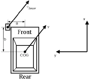
The Figure 3-10 shows a vehicle in rectilinear motion: the velocity measured by the sensor ( ) is the same with the vehicle velocity calculated at the COG (3.1):

Figure 3-10 – Rectilinear vehicle motion

It is possible to see again the vehicle coordinate system defined in 2.2.2., in which the x-axis points to the front of the vehicle, the y-axis to the left and the z-axis upwards (right hand system).

17

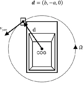
Case 2: Pure yaw vehicle motion

With a pure yaw motion around the centre of gravity as rotational centre the vehicle velocity should be “0”, as shown in the following Figure 3-11. As the sensor is not mounted in the COG, it will measure a velocity that is dependent on the yaw rate r and the position in relation to the COG. The position of the sensor in the COG is (3.2):

Figure 3-11 – Pure yaw motion

The velocity that the sensor measures can be calculated as follows (3.3):

Case 3: Combined motion

The normal motion conditions are a superimposition of COG velocity v and the velocity caused by yaw , therefore the speed measured by the sensor is (3.4),(3.5):

18

3.1.5.2. Sensor positioning

The sensor can be mounted at one side of the vehicle or in the front of it; in this case a right side mounting is chosen, as shown in Figure 3-12. It is positioned in correspondence to the COG, so that .

Figure 3-12 – Installation of CORREVIT® sensor for mounting at the vehicle side

The previous equations are therefore simplified (3.8),(3.9):

The definition of the vehicle’s COG requires the use of a scales which can measure the weight distribution on each wheel.

19

3.2. Proving ground vehicle tests

3.2.1. Introduction

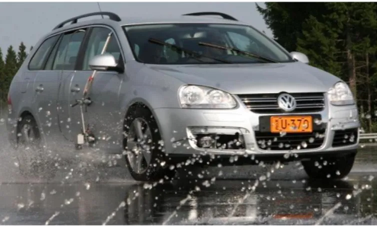
The research vehicle was tested in the Nokian Tyres test track located in Nokia [14] (Figure 3-13). Different manoeuvres with different set of tires were tested on it.

Figure 3-13 – The Nokian Tyres proving ground [14]

In the proving ground was possible to conduct steady-state cornering manoeuvres, with steering angle and longitudinal speed imposed by the driver. All the manoeuvres were tested on dry asphalt conditions, with the friction coefficient between ground and tire assumed to be as one.

3.2.2. Description of the manoeuvres

All the manoeuvres were run with the ESP (Electronic Stability Programme) switched off. Two kinds of manoeuvres were tested:

the first one was obtained in the section 6 and 7 of the proving ground (Figure 3-13) and consisted of a double-lane change manoeuvre at a start speed of 108 km/h. This kind of test is representative of the transient lateral behaviour of a vehicle and it is necessary to validate the suspension model of the vehicle (it will be described in chapter four).

20

the second one was obtained in the circle 2 and it was the so called “Steering pad”: the driver follows a constant radius (40 m) increasing slowly the longitudinal speed and changing the steering angle. Both clockwise and counter clockwise manoeuvres were obtained. This test allows to easily representing the understeering or oversteering behaviour of the vehicle. However, it’s fundamental to remember that in normal cars, i.e. with two axles and open differential, trying different steady-state manoeuvres shouldn’t have any influence on the handling curve of the vehicle which remains the same [3].

3.2.3. Tires tested

3.2.3.1. Choice of the tires

The possibility to change the understeering and oversteering behaviour of the vehicle was also investigated considering two different set of tires, both for winter conditions:

Nokian WR G2 205/55R16 91 H, not studded: the tread has an asymmetrical shape designed to remove slush and water and guarantee perfect driving conditions in the weather of Central Europe (Figure 3-14).

Figure 3-14 – Nokian WR G2

Nokian WR G2 205/55R16 91 V Run Flat, not studded: it’s a particular tire with reinforced sidewalls that are capable of bearing the weight of the car in

21

case of flat condition (Figure 3-15). Therefore it’s possible to drive about 50 km on an empty tire, with a maximum speed allowed of 80 km/h: the Run Flat tire behaves as a spare tire [15], [16].

Figure 3-15 – Construction characteristics of a Run Flat tire [16]

For practical reasons, in the next parts of the thesis the two set of tires will be distinguished as follows: WRG2 for the Nokian WR G2 205/55R16 91 H and simply RF for the Nokian WR G2 205/55R16 91 V Run Flat.

3.2.3.2. Influence of inflation pressure

Increasing the tyre inflation pressure leads to a reduction of the dimensions of the contact patch; moreover, experiments show that, increasing the inflation pressure, the friction coefficient between tyre and asphalt is slightly reduced (usually this physical phenomena is modelled as shown in 3.3.1.4 by equations (3.18) and (3.19)). Therefore, to increase the road holding of the vehicle it’s possible to think to a reduction of the inflation pressure; on the contrary, a deflated tire can easily warp. A compromise between these two opposite needs is to be found [3].

It’s worth remembering also the influence that inflation pressure has on the cornering stiffness Cα: increasing the inflation pressure starting from a low value (about 1.3 bar) leads to a rise of the cornering stiffness but only until when a limit inflation pressure is reached (about 2.0÷2.2 bar). After this value the cornering stiffness starts to decrease.

Furthermore, the so called “inflation pressure” that is considered in literature usually refers to the initial conditions of pressure, measured at room temperature.

22

During the test, a considerable increase of the tire pressure can be noticed, caused by heating of the tire due to the slip with the asphalt.

Three pressures were kept in consideration during the tests: for WRG2 tires were used 1.8 bar and 2.2 bar, and for Run Flat tires were considered 2.2 and 3 bar. The aim was to show the different behaviour of the two set of tires in terms of cornering stiffness and tire vertical stiffness k.

3.2.3.3. Set of tires

The following combinations were tested on the proving ground (Table 3-2):

Combination

Front axle

Rear axle

Tire Pressure

(bar) Tire Pressure (bar)

1 WRG2 2.2 WRG2 2.2 2 RF 2.2 WRG2 2.2 3 WRG2 2.2 RF 2.2 4 RF 2.2 WRG2 1.8 5 RF 3.0 WRG2 1.8 6 RF 2.2 RF 2.2

Table 3-2 – Six combinations of tyres tested

In particular, the double-lane change manoeuvre was performed with the second combination, whereas for the steering pad all the different combinations were tried.

3.2.4. Tires measurements and results

3.2.4.1. Introduction

In order to study the mechanical behaviour of the tire and to create a model which is as close as possible to the reality, an experimental analysis made on single wheels

23

is required. These types of tests are normally performed making the tire run on a machine which can be a road simulator or a rolling rig. The latter consists of a “drum” coated with an artificial road surface or a replica of a real road surface [17]. Tests on a rolling rig have the major advantage of controlling a certain number of parameters which cannot be controlled on a test truck (e.g. tire temperature, load, brake torque, etc.).

The tire test rig used for the master thesis has been designed in the Laboratory of Automotive Engineering [18] and it’s shown in Figure 3-16.

Figure 3-16 – View of the tyre test-rig [18]

3.2.4.2. Mechanical structure

The rig can measure all common sizes of passenger car with normal tyres and rim. The test tire rolls against the dynamometer drum: it has a diameter of 1219 mm and can reach a maximum circumferential speed of almost 200 km/h. The drum is coated with a grip tape which roughness is about P60 according to the ISO/FEPA Grit designation [19]. The test rig can measure all forces and moments acting between the tire and the dynamometer drum . The maximum wheel load is 7000N, the slip angle of the tire can be adjusted between

24

+/-10 degrees and the camber angle between +/-4 degrees. There is also a disc brake in the hub, so that in every moment is possible to brake the tire.

As shown in Figure 3-17, the rig consists of a huge slewing ring which allows slip angle rotation, a frame made by welded steel beams, knuckle eyes that connects the slewing ring and the frame and allows camber angle rotation. A linear guide allows tire translation in vertical direction; furthermore, thanks to the presence of a spring and a shock absorber, it’s possible to adjust the tire wheel load. Hydraulic cylinders make all movements of the rig (not showed). The measuring system consists of six force transducers, potentiometers to evaluate camber and slip angle and an incremental encoder that measures the rotation speed of the tyre (not showed).

Figure 3-17 – Characteristics of the test rig

3.2.4.3. Test results

As explained in 3.2.3.2., two different set of tires were tested: the WRG2 tires were tested at 1.8 bar and 2.2 bar, and for the RF pressures of 2.2 bar and 3.0 bar were chosen. In this section, the pictures for measured lateral forces against the tire slip angle are shown. It’s worth to remember that the following graphics represent only a small part of the data amount which is possible to extract from the test rig.

25

Moreover, during the tests were considered four different vertical loads: 1950, 3450, 4950 and 6450 N. Those values clearly represent how the lateral force can change at constant values of slip angle; the same values were also used in the creation of the empirical equation called “Magic Formula” which models the tire behaviour. Figure 3-18 shows the lateral forces of a single WRG2 tyre at pressure of 1.8 and 2.2 bar; Figure 3-19 shows the same relation for a RF tire at pressure of 2.2 and 3.0 bar:

Figure 3-18 - Lateral force versus slip angle at different wheel loads, WRG2 1.8 bar and 2.2 bar

Figure 3-19 - Lateral force versus slip angle at different wheel loads, RF 2.2 bar and 3.0 bar

26

The following pictures from Figure 3-20 to Figure 3-23 show, for different loads, how the lateral force vs slip angle curve changes when the pressure is modified: from 1.8 bar to 2.2 bar for the WRG2 tyre, and from 2.2 bar to 3.0 bar for the RF tyre.

Figure 3-20 – WRG2 tyre,lateral forces vs slip angle, comparison between different pressure; 1) Load: 1950 N; 2) Load: 3450 N

Figure 3-21 – WRG2 tyre, lateral forces vs slip angle, comparison between

27

Figure 3-22 – RF tyre,lateral forces vs slip angle, comparison between different pressure; 1) Load: 1950 N; 2) Load: 3450 N

Figure 3-23 – RF tyre, lateral forces vs slip angle, comparison between different pressure; 1) Load: 4950 N; 2) Load: 6450 N

Not a big difference is noticed changing pressure in the WRG2 tyre, especially because the modification is slight (from 1.8 bar to 2.2 bar); a more important variation is possible to notice in the RF tyre, where the modification of pressure is from 2.2 bar to 3.0 bar.

28

3.3. Modelling environment

3.3.1. Tire model

3.3.1.1. Introduction

When a vehicle model has to be created, one of the most important tasks is the generation of a realistic tire model. In fact, the quality of a vehicle dynamics simulation is heavily influenced by the capabilities of the tire model. In the following paragraphs is described the importance of using tire empirical model and the basic outline of one of the most known in literature called Magic Formula, which was developed by H. B. Pacejka.

3.3.1.2. Considerations on the choice of empirical models

With the aim of describing the behaviour of the tire, in particular the trend of the lateral force as a function of the slip angle , semi-empirical formulas can be used. In this case, the goal is simply to seek formulas that, while not having any connection with physical reality and the real behaviour of the tire, can describe the trend of experimental forces and moments, even if in an approximate way.

The definition of an empirical model is not, in the case of the tire, a simple problem of approximation of functions with unknown analytical expression: there are additional constraints to observe, instead. It has considerable importance, for instance, how to approximate the first derivative of the function, rather than having fluctuations in the gradient which are not present in reality. Ultimately this is equivalent to have constraints on the second derivative, and this makes the problem of approximation more delicate: the classical “least square method” cannot be implemented in this case because it doesn’t provide accurate approximations of the derivatives [3].

29

3.3.1.3. Magic Formula basic description

The most widely used description of the experimental trends of and is that given by Pacejka, better known under the name Magic Formula. Pacejka proposed the formula [20] (3.10):

with (3.11), (3.12):

where is the output variable which is defined as the longitudinal force

if is defined as the slip ratio , or as the lateral force if is defined as the side slip angle . The remaining variables of the Magic Formula describe the following coefficients: stiffness factor shape factor peak value curvature factor horizontal shift vertical shift

which must be set in order to obtain the desired trend, or one that is closest to experimental results.

The Magic Formula typically produces a curve that passes through the origin , reaches a maximum and subsequently tends to a horizontal asymptote. For given values of the coefficients B,C,D and E the curve shows an anti-symmetric shape with respect to the origin (Figure 3-24) [21]. To allow the curve to have an offset with respect the origin, two parameters for shifting and have been introduced: a new set of blue coordinates X and Y is therefore created.

30

Figure 3-24 – Curve produced by the equations (3.10), (3.11), (3.12) [21]

Considering the Figure 3-24 as representative of the lateral force characteristic, it is possible to notice the meaning of the previous coefficient. D represents the peak value for ; the slope at the origin is given by (3.13):

C determinates the shape of the curve, instead B is used to fix the slope at the origin and that explains this name. The factor E is introduced to control the curvature at the peak and at the same time the horizontal position of the peak . A good tire model has to keep in consideration also the influence which vertical load has on longitudinal and lateral force. For this purpose it’s possible to introduce the normalized change in vertical load as (3.14):

In the previous formula the quantity represents the nominal load acting on the wheel.

A more complete expression of the Magic Formula is given in the next section, which takes into account also the influence of the wheel camber angle .

31

3.3.1.4. Lateral force (pure side slip)

The field of interest of the thesis is only limited to the visualization of the lateral force between tires and asphalt. Therefore all the quantities in the Magic Formula (3.10) are rewritten with the “y” subscript (3.15):

The equation (3.15) gives force solely as a function of the slip angle . Since tire lateral force is a function of both slip angle and vertical load, the equation (3.16) through (3.25) were used to account for vertical load. The new full formulation will have the coefficients , , , function of the vertical load, whereas is a function of both vertical load and slip angle:

About the previous equations the following consideration can be expressed:

All the six Magic Formula coefficients ( , , , ) are now rewritten as function of new 18 parameters that are: , , ,

, , , , , , , , , , , ,

32

These are curve-fitted parameters which show the relationship of the Magic Formula coefficients to the vertical load and camber angle. Their use will be necessary in the used modelling environment, the car simulation tool “CarMaker®”.

The influence of camber angle is neglected, as it was not possible to evaluate it during the creation of the vehicle model. Therefore, all the previous equations are simplified (it is not necessary anymore to take into account the

parameters , , , , , );

The coefficient is function of the vertical load according to the empirical equation (3.18), where the lateral friction parameter (equation (3.19)) appears.

The coefficient given by the equation (3.23) is the result of another empirical equation that allows to calculate the slope at the origin of the lateral force characteristic (3.26):

is function of three parameters as shown in the equation (3.21), (3.22).

3.3.1.5. Results

The eighteen parameters function of the Magic Formula coefficients are extracted from experimental data from real tires described in 3.2.3.. To obtain this, the Curve Fitting Tool (cftool) of Matlab® is used. To determine the parameters an optimization routine is used. The aim is to minimize the error between the measurement and the Magic Formula model.

Figure 3-25 and Figure 3-26 show a comparison between experimental data and Magic Formula, respectively for WRG2 tire 1.8 bar, WRG2 tire 2.2 bar, RF tire 2.2 bar, RF tire 3.0 bar; in black is represented the Magic Formula:

33

Figure 3-25 - Comparison between experimental data and Magic Formula, WRG2 1.8 bar and 2.2 bar

Figure 3-26 - Comparison between experimental data and Magic Formula, RF 2.2 bar and 3.0 bar

3.3.2. Creation of the handling diagram

3.3.2.1. Introduction

In this section how to get handling diagrams from the test car is shown. After having acquired all the experimental data from the sensors, these are processed with the aim of plotting experimental handling diagrams. Thanks to them, is therefore

34

possible to show the understeering-oversteering behaviour of the vehicle, as already mentioned in Chapter two. In particular, six different set of tires were tested, so that six different handling diagrams are plotted. Furthermore, they will be used as a reference for the creation of a vehicle model in the simulation software CarMaker. This will be clearly shown in the Chapter four.

3.3.2.1. Diagram plotting method

Four different signals are necessary to plot a handling diagram. These are:

the steering angle extracted from the steering angle sensor as shown in 3.1.2.;

the longitudinal velocity u obtained by the optical sensor CORREVIT® S-350 as shown in 3.1.5.;

the yaw rate signal r ; as shown in 3.1.4., it is possible to get this from the Golf yaw rate sensor;

the steady state lateral acceleration ; this can be evaluated from the lateral acceleration sensor shown in 3.1.3. or it can be simply obtained as product of two quantities: u and r, as shown in equation (2.9). This second approach will be always used during the tests.

However, as shown in 3.5.1.1., it is necessary to correct the speed signals obtained from the CORREVIT® sensor: in particular, it’s necessary to know the quantity “t/2” shown in Figure 3-27 which represents the lateral distance between the CORREVIT® sensor and the COG of the vehicle. The Figure 3-27 not only shows the distance t/2 but also the height of the COG h, both fundamental for the sensor positioning:

35

Figure 3-27 – Height if the COG and distance t/2

By means of measurements, the quantity t/2 is calculated and it is: t/2 = 0.993 mm. It is now possible using the equation (3.8) to correct the signals from the CORREVIT® sensor (3.27):

Finally, the handling diagram is given by the equation (2.14) as shown in 2.3.. For the set of tires presented in 3.2.3.3., the following handling diagrams are obtained (Figure 3-28):

36

Figure 3-28 – Handling diagram obtained with different set of tyres

From the previous handling diagrams, one of the most relevant results is that, mounting a RF set of tire at front axle can heavily change the directional behaviour of the vehicle. There is almost a separation between the handling diagrams which have WRG2 at front (magenta and blue in Figure 3-28) and RF at front (red, black, green and yellow in Figure 3-28). Therefore, is possible to distinguish two different groups of diagrams. Within these two groups, mounting a WRG2 set of tire at rear axle, the behaviour of the vehicle is more understeering (i.e., in the first group, the blue set gives a more understeering behaviour than the magenta; in the second group, the black set gives a more understeering behaviour than the red).

The last consideration regards the tire inflation pressure: increasing front tire pressure the vehicle becomes more understeering (i.e. the yellow set gives a more understeering behaviour than the green); on the contrary, increasing the rear pressure, the vehicle tends to be oversteering (i.e. the black set gives a more oversteering behaviour than the yellow one).

37

According to the previous considerations, the WRG2 front 2.2 bar – RF rear 2.2 bar gives the less understeering behaviour; the RF front 3.0 bar – WRG2 rear 1.8 bar gives the more understeering behaviour of the vehicle.

By considering all the results obtained, in the next chapter a complete car model will be created thanks to a simulation software. All the manoeuvres tested at Nokia proving ground will be simulated, so that the model will be validated. It will be possible to recreate the previous handling diagrams and add new ones considering a further change in tires pressure.