TESTING THE PMA32

(1)

60

CHAPTER 3

TESTING THE PMA32

3.1 PMA-32 CONFIGURATION

3.1.1 HOW TO CREATE A CROSS-CONNECTION

To configure and test the behavior of the PMA-32 we have connected 2 PMA’s to each other on a ring which, this way, can be considered a kind of simple point-to-point link. One PMA is located at the Department Of Information Engineering c/o University of Pisa, while the other is in San Cataldo’s CNIT - with a link on the distance of about 23,5 Km. Selecting “Connections…” on the Connections menu we’ll get a new window:

considering the “CROSS CONNECTION DETAILS” menu we can notice that the CORE of our PMA consists of 2 lines, on which the signal will be sent - West and East, and that each line has some configured wavelengths which will be added or dropped as we need. For this first experimental connection our system involves 4 nominal tributaries at the source:

- Tributary 19 which carries the 192.60 frequency, having a protection line; its transponder accepts SDH or Sonet tributaries only.

- Tributary 23 which carries the 192.70 frequency, with no protection in it; accepting SDH/Sonet only.

- Tributary 24 which carries the 193.50 frequency, with no protection too; accepting - as the above transponder - SDH/Sonet only.

- Tributary 21 which carries the 192.80 frequency; accepting also Gbit Ethernet traffic.

As for the payload type, we can select each tributary on the sub-rack menu and choose it directly using the PORT – PORT CONFIG. menu and deciding what kind of payload to add and drop.

While the first 3 tributaries are shown in Figures 3.1 & 3.2 as already configured with potential type and protection type, but not really active on the link because no traffic is sent on them - we are going to work on the last one to create an active cross-connection, showing the easiest way to do it.

We are going to configure just the 192.80 tributary because it is the only one to correspond to a transponder which also accepts traffic from any optical Gbit Ethernet network.

Selecting either Line West (Figure 3.1) or Line East (Figure 3.2) in the NE SOURCE - CORE menu we’ll see the following expected things:

-192.60 tributary is shown in both lines as it has a protection.

-192.70 is only shown in line west – and transmitted on one direction only, as expected. -193.50 only in line east, and transmitted on line east for the same reason.

Plus, we can notice a 193.10 tributary - coming from the PMA situated at the other end of the link c/o the CNIT structure – shown in both lines as it has got a protection in it;

moreover this frequency’s transponder accepts Gbit Ethernet traffic too, so it has a great potential for implementing a real multiplexing system, together with the 192.80 frequency.

(2)

61

As already highlighted, 192.80 is the frequency we are going to consider now to create a cross-connection, as there’s no configured type or protection type at the moment, as we can notice in the 2 mentioned pictures.

Figure 3.1 – NE Source’s LINE WEST showing our 192.80 tributary

Figure 3.2 – LINE EAST, showing the 192.80 frequency again

A very useful thing before starting our configuration is to explain the way a potential ring can be seen by an operator on our system software.

(3)

62

When we select a potential traffic on the NE Source’s LINE WEST we’ll notice only a LINE EAST on the NE Destination’s CORE, and this is due to the way our PMA works: it sends an optical channel (or better many ones, considering that it manages a multiplexed signal) on the ring using the TX West terminal, and finally it receives the signal coming back from the ring on the RX East terminal. The same thing happens to the eventual protection ring which goes starting at the TX East terminal and closing the ring at the RX West terminal. Logically talking the originated topology seems two rings rotating on different directions. This explanation will happen to be very useful to the reader, considering that the Marconi PMA’s software seems to be a little hermetic to comprehension from time to time, when considering the tributaries’ indications in the menus

To have a complete view of our point-to-point link, we can use a great potentiality of our software: the remote management – accessible from the main menu.

In Figure 3.3we’ll show the window obtained when selecting REMOTE MANAGEMENT. It is clear in the picture that the system automatically recognizes the addresses belonging to the other PMA’s on the ring – and this will facilitate our remote connection.

Figure 3.3 – How to have access to other PMA’s in Remote Mode

Figure 3.4 – The configured transponders on the 2nd PMA, shown in Remote Mode

Let’s also underline that in remote mode we are capable to do more or less everything as if we were directly connected to the system we have logged in to.

(4)

63

We’ve also inserted Figure 3.4, that shows the tributaries which are already configured in the 2nd PMA, c/o the CNIT structure.

The present situation only contains two frequencies (192.80 and 193.10) for which transponders have been configured, because the remaining two transponders (192.20 and 192.30) only accept SDH/Sonet traffic and not Gbit Ethernet optical systems.

The 192.80 happens to be ideal for the traffic we want to send over the link from our PMA. The first step to create a cross-connection on the ring is the selection of the tributary we are interested in on the NE SOURCE, in the SUBRACK1 menu (so we’re talking about transponders) – in our case it is the tributary #21 which carries the 192.80 THz component: actually we have got one transponder at each side of the ring that works at this wavelength, as already seen.

After this, we also select 192.80 – the same wavelength – on the NE DESTINATION, choosing LINE WEST for example.

After investigating the way the transmission takes place, we must immediately say that the protected 192.80 transponder seems to work only if configured with protection, that is to say with a double ring transmission, otherwise no connection seems to be obtained. So it is not important whether to select Line West or East in the destination’s CORE, because in both cases the signal, after activating the protected line, will be sent on two directions – so up to West and East destinations.

This procedure is simply shown in Figure 3.5.

Figure 3.5 - First step for the cross-connection: selection of the 192.80 frequency up to the West RX terminal

When the 192.80 has been highlighted on both sides of the menu we can select CREATE CROSS CONNECTION, BIDIRECTIONAL on the PATH menu as shown in Figure 3.6.

(5)

64

Figure 3.6 – Selecting the Creation of the Cross-connection

A little window to confirm the given data is shown: just choose OK – and the cross-connection between source and destination has been created.

We immediately notice that in the left side menu “NE source - CORE – LINE WEST” the 192.80 tributary is indicated with the “BIDIRECTIONAL” type of connection. The same indication will be shown on the “NE destination – CORE – LINE WEST”.

The result is shown in Figure 3.7.

(6)

65

A second protection ring can be enabled, once closed the CORE menu at the NE destination, by selecting on the PATH menu CREATE SNC PROTECTION – as shown in

Figure 3.8 for making the procedure more immediate.

The protection is useful to send the same signal on two lines. Just notice that without activating the protection the PMA-32 seems not to work properly.

Figure 3.8 – First step to create SNC protection

A window as the one shown in Figure 3.9 will contain some default values to activate the protection ring. Click OK.

(7)

66

We’re going to explain the specific values better later in this chapter, because the SNC protection needs some selections according to the way our link has to work.

“INTRACARD SNC PROTECTION” will be shown (Figure 3.10), demonstrating that the desired double ring transmission has been created.

Figure 3.10 – Protection has been activated

At the end of this procedure we’ll have our result (understandable in Figure 3.11):

Figure 3.11 – Result of the procedure: 192.60 and 192.80 tributaries have their protected cross-connections (indicated with “Bidirectional” and “Intra Card”)

(8)

67

Between the two PMA’s connected on the ring we have now 2 tributaries – the 192.80 and the 192.60 – that have one bidirectional link plus one protection bidirectional link.

3.1.2 HOW TO DELETE A CROSS-CONNECTION

To delete a cross-connection one can select the desired tributary and choose DELETE CROSS CONNECTION in the PATH menu.

First of all it’s necessary to select DELETE SNC PROTECTION in the same menu, if the protection has been enabled for that tributary.

3.1.3 HOW TO CREATE A SIMPLE PASS-THROUGH

Another possibility we have is to create a pass-through – for example for the 193.10 wavelength, which is sent on the link by the second PMA, situated about 35Km away from the one we’re analyzing.

The first step to follow is selecting, as in the cross-connection, the 193.10 frequency, but this time not in the SUBRACK menu: we have to highlight it (as shown in Figure 3.12) both in the CORE – LINE WEST menu at NE source and in the CORE – LINE EAST at NE destination, thus meaning that we want this tributary, when received by our PMA on line west, to be immediately sent on line east – same thing on the other direction.

Figure 3.12 – First step to activate a pass-through

Second step: on the PATH menu we shall select CREATE CROSS CONNECTION – Bidirectional, as shown in Figure 3.13.

(9)

68

Figure 3.13 – Creation of the desired pass-through

Differently from the configuration of a cross-connection, this time we’ll notice that next to the frequency we’re working on “Line East” or “Line West” will be displayed, instead of the tributary number: we have created a pass-through – which brings, as said, the signal received from the NE destination’s Line East to the NE source’s Line West without working on it (Figure 3.14).

(10)

69 3.1.4 HOW TO DELETE A PASS-THROUGH

To delete a pass-through one can select the desired frequency on both NE source and NE destination and choose DELETE CROSS CONNECTION in the PATH menu.

In this case it’s unnecessary to select any DELETE SNC PROTECTION option, as it should be done for a cross-connection with protection features.

3.1.5 HOW TO CONFIGURE/UNCONFIGURE A TRANSPONDER

Let’s start now explaining the procedure necessary to configure the transponder units when a card is moved from a slot to another one.

First of all, as the PMA software is not so elastic during the procedures directly involving the hardware, it is important that you follow what we’re going to show step by step. We’ll try to use a standard procedure, useful not to face additional problems during the configuration/un-configuration.

Let’s try to change the position of the T5-6 and T7-8 transponders, moving the cards to the new T9-12 slots.

We’ll select UNCONFIGURE (Figure 3.15) for the T5 and T7 tributaries (that is to say T 5,6,7 and 8 – as the two transponders are protected).

Figure 3.15 – First step to UNCONFIGURE T5 and T7 transponders

After this we immediately open the CONNECTIONS menu, because we’re going to delete the cross connections involving the two considered transponders.

In Figure 3.16 we see the DELETE SNC PROTECTION option for the T7 tributary – alias frequency 192.8.

(11)

70

Figure 3.16 – DELETE SNC PROTECTION option for the T7

The same thing will be done for the T5 transponder.

As you can see, the cross connection can be deleted only after the elimination of the protection – if you want to learn more about this you can read above, in the section about HOW TO CREATE A CROSS CONNECTION. In the next picture (Figure 3.17) we show how to delete the desired cross-connection, once deleted the SNC protection.

(12)

71

Now that we have eliminated every single cross-connection for the two frequencies are transponders are related to, we can click on MODIFY CABLE (Figure 3.18), in the inferior part of the Local Craft Terminal window – so to be able to delete the link between a certain frequency and the T5,6 / T7,8 transponders.

Actually in our case we’re going to use the 192.8 and 193.5 frequencies in slots different from the 5-8 considered until now.

Figure 3.18 – MODIFY CABLE option

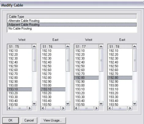
Selecting MODIFY CABLE you’ll have three possible choices (as shown in Figure 3.19): - NO CABLE ROUTING

- ADJACENT CABLE ROUTING - ALTERNATE CABLE ROUTING

The first option will be used in our case, because we don’t need to replace the moved transponder with a new one, so the slot is to be un-configured until we need it again. Adjacent cable routing is the possibility we will select because we are using protected transponders, so we need two consecutive slots to be connected to a single frequency – in our case 193.1 and 192.80 for our two transponders respectively.

Alternate cable routing is a third option that can be used when we use transponders which have no protection on them.

In the following picture (Figures 3.19, 3.20) we must select NO CABLE ROUTING for the T5 and 7 slots, as already said, because we’re moving the two cards to new slots, as we are going to see in the next page. Selecting “No cable routing” we’ll get a grey window showing we’re not using those slots at the moment.

(13)

72

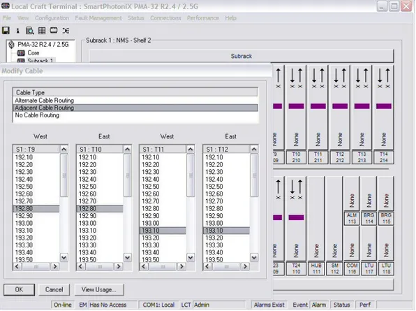
Figure 3.19 - Actual ADJACENT CABLE ROUTING choice in MODIFY CABLE window

Figure 3.20 – Final NO CABLE ROUTING choice

Clicking Ok and getting back to the usual Local Craft Terminal we will notice how the considered slots are now shown in violet as many other slots (Figure 3.21).

We’re going to choose T9,10,11,12 slots for our two cards, and the procedure we show in the flowing pictures is the same we have already used, but this time we’ll select ADJACENT CABLE ROUTING in the MODIFY CABLE window (Figure 3.22).

(14)

73

Figure 3.21 – T5,6,7,8 slots are now with no frequency indicated

(15)

74

Selecting the VIEW CARDS mode we can notice that the two protected transponders are now shown in grey, meaning that the software has detected they have been inserted in the PMA-32.

What we finally need to do is clicking ADOPT to let the software accept the new cards.

Figure 3.23 – ADOPT function

One thing that is not immediate to remember but very important when trying to configure the system, especially when the link involves many PMA’s, is that - every time we change the position of a card facing the procedure shown above – the software choose a default “STM” transmitted payload for the add port. In Figure 3.24 we can see how to verify this matter.

(16)

75

Let’s highlight that if we do not select the right payload type (in our case Gbit Ethernet) we’ll have no traffic passing through the PMA-32.

So it is important to verify this feature every time we change something in the Sub-rack slots, not to have doubts when eventual alarms are shown and there are more problems in the system.

In Figure 3.25 we see the many options we have for the payload type: in this case, as said, we assume Gbit Ethernet as the right type.

Usually when moving a card the only default transmitted payload which is automatically changed is the ADD port one, but it’s a good habit to verify that even the DROP port payload is still indicated as Gigabit Ethernet or as it is expected to be.

Figure 3.25 – Gigabit Ethernet payload type

If an operator forgets to select the right payload type, an alarm indicating “Payload Type Mismatch” will appear and the traffic will not run through the system.

In the next sections we’re considering the most common activities to test the PMA32, and the way this apparatus can be used to multiplex different signals using different paths.

(17)

76 3.2 “ANALOGUE MONITOR DISPLAY”

The analogue monitor function is useful to view the transmission and reception power values on the West & East TX / RX lines and in the various transponders managing the different wavelengths.

In the LOCAL CRAFT TERMINAL window there is the possibility to select “ANALOGUE MONITORING – Display” right-clicking on a single transponder in the sub-rack or a single component in the core, thus getting the relevant parameters – which change depending on the particular component we choose.

Let’s also say that the Analogue Monitor window is useful for another reason: there is the main optical stuff used in the hardware (for example in the TX or RX, or in transponders) clearly indicated – and we’re also going to explain a little about it as soon as we analyze the single components.

The selection to activate the Analogue Monitor Function is shown in Figure 3.26.

Figure 3.26 – How to activate the ANALOGUE MONITOR function

3.2.1 ANALOGUE MONITORING ON A SINGLE PMA

Using only 1 frequency

The following sections will be explaining the Analogue Monitoring function when transmitting traffic on a frequency onto either a single PMA or a point-to-point link.

In the next parts of this book we’ll analyze what changes when we use more than 1 frequency, so creating a real multiplexed signal and a real multiplexing topology, comparing the values we’ll get with the values we are obtaining in the next pages for a single cross-connected frequency.

As we are going to test the way a ring connecting some PMA’s works, the first step to take is determining the most important parameters about a single PMA-32, connected neither to others nor to the fiber link that we’ll consider later in our analysis (the one connecting the Engineering faculty to the CNIT block).

The first thing we have to do is separating the PMA from the 4 fiber cables that connect us to the ring throughout the city-center of Pisa and connecting the West TX with the East RX,

(18)

77

and the East TX with the West RX, so making the PMA be connected only to itself with something like a fiber micro-ring.

In the part of this book regarding the tests with the AX4000 Traffic Generator & Analyzer there is a section regarding the single PMA used in this analysis with particular attention to its performance while delivering packets.

Before looking at the Analogue Monitor Windows, just a short explanation about the alarms we can notice when connecting the considered PMA with itself using 2 fiber cables – as we highlighted above. Figure 3.27 shows what we get when selecting REAL TIME ALARMS in the VIEW menu.

Figure 3.27 – ALARMS obtained using a single PMA

It’s useful to compare these alarms with the alarms which used to appear before extracting our single PMA from a point-to-point ring already configured with 2 PMA’s (Figure 3.28).

(19)

78

The alarms highlighted in blue are just warnings. The ones we’re interested in are the yellow minor severity alarms and the red critical severity alarms.

As we can notice, the 193.10 tributary has been alarmed in yellow with “Connected Path Absent” (one alarm for each line, as it’s a protected transponder), because it had been configured to be in cross connection with the PMA at CNIT – and this cross-connection is not up now.

Besides the 192.60 “Connected Path Absent” indication has disappeared, because while in the point-to-point link there were no transponders at CNIT capable to work at the 192.60 frequency, now we could have the potentiality to use our protected transponder for add/drop functions.

The remaining 192.70 and 193.50 tributaries are shown also as red now (first picture of the 2) with the indication “Present Path Unconnected” because their transponders generate unprotected lines, differently from what happens to the 192.60 frequency; the configured cross-connection for the 192.70 and 193.50 don’t work anymore without a 2nd PMA, so we can solve the red alarm by deleting the existing cross-connections and configuring a pass-through for the 2 involved tributaries.

For the pass-through creation just have a look at the apposite section in the PMA-32 CONFIGURATION paragraph.

And last, the Loss Of Signal Alarms refer to the transponders which are not connected to any fiber cables at the moment – as for the present situation they have been partially manually disabled because it’s obvious that there are some frequencies we are not going to use during our tests.

TEST #1 – PMA not yet connected to the AX4000 Traffic Generator

We’ll start the actual testing by viewing the TX and RX terminals’ analogue monitor windows (we’ll consider the West line only – because the East one is just the same), going on with the 192.80 tributary’s one, which will be the object of our analysis even for the next test regarding two PMA’s connected on a point-to-point link.

In Figures 3.29 and 3.30 we analyze respectively the TX and RX power values obtained on the West Line simply using the PMA not yet connected to the AX4000 Traffic Generator.

(20)

79

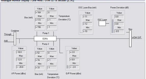
The picture also shows the PMA TX Section’s internal composition - as we are explaining in the following lines.

Added channels and pass-through channels will be treated by the 8:1, 16:1 or 32:1 COMBINER, which produces the signal sent to the EDFA amplifier.

The latter amplifies the signal adding +20dB; as we can see in Figure 3.29 -16 dBm becomes +4 dBm after the EDFA treatment.

The indication shown as “WDM O/P” represents the Multiplexed signal obtained using the traffic coming from the Add/Drop Unit (containing the Combiner) and the signal coming from the Channel Control Unit – and finally adopting the OSC Laser to transmit onto the fiber cable.

Figure 3.30 – RX section @ PMA not connected to the AX4000

As for the RX Section picture shown above (Figure 3.30), we see the “WDM I/P” signal – still to be de-multiplexed.

The DEMUX role is solved by a SPLITTER, which receives the signal coming from the pre-EDFA amplifier. And finally the signals dropped by the splitter are sent onto the needed tributary’s transponder.

(21)

80

Figure 3.31 shows the power values obtained for the 192.80 tributary: from this picture we can easily work out the behavior of the transponder: the client input signal at whatever wavelength, through an opt-electric transformation, pilots the WDM laser.

Up to here the process is indicated in the mentioned picture.

To have a complete idea of what happens later, the WDM laser sends a new optical signal to the Add/Drop Unit, so having access to the TX Line Unit, and to the fiber link through the created multiplexed signal, containing our single WDM laser-generated frequency. Coming back to our 192.80 Analogue Monitoring Window, as we can notice the I/P Power field is -33,4 dBm – thus indicating there’s no client connected, as expected.

Instead the O/P Power values on the transmission lines, and the I/P Power values on the receiving lines seem to be properly measured – it seems that, even with no connected tributary and with no traffic being sent, the TX and RX lines have powers going through the system.

We’ll see if these values match with the ones measured when traffic is sent throughout our PMA.

As for the tributaries which have been configured as a pass-through, and to which there’s nothing connected that can be passed through, we get -54 dBm in the I/P Power field and -18.8 Dbm in the O/P Power field, signaling there’s no optical channel getting through at those frequencies.

TEST #2 – PMA now connected to the AX4000

Connecting the PMA’s tributary #21 (the usual 192.80 frequency) to the AX4000 we’ll get the same TX/RX Section’s Analogue Monitor Windows.

The only different thing we get is the following Figure 3.32 result (regarding the tributary transponder):

the I/P Power field is not -33,4 dBm as above, but we have a new -4.4 value – actually we’re connected to the Traffic Generator & Analyzer, so the PMA notices that, producing an expected power value.

(22)

81 TEST #3 – PMA connected to the AX4000, with traffic on 1 frequency

What we want to verify with this test is the range of values we can get when we generate traffic onto the PMA, comparing the data with the power ranges obtained above – so we’ll be able to know if there are substantial differences and if our Analogue Monitor Display can be useful for analysis.

Let’s send for example 1600 byte periodic IP packets using the AX4000 Traffic Generator, selecting 100% as Max load/fixed length. As we are using a single PMA and the ring is just a very short fiber cable we expect the packet transfer delay to be not so big as value. Actually the situation is just as predicted (Figures 3.33, 3.34).

The delay is about 3.5 usecs. The easiest way to judge this result is having another test on the AX4000 only, so valuating the delay due to the Traffic generator/analyzer – we’ll face this test in the section about the AX4000 analysis. The same kind of packet transfer delay is obtained when we try to send smaller packets such as 64 bytes packets.

Figure 3.33 – Packet Transfer Delay obtained on a single PMA with 1500 byte IP packets

(23)

82

Here below, we just show the results obtained in the Analogue Monitor Display generating traffic (Figures 3.35, 3.36, 3.37).

Figure 3.35 – TX section @ PMA connected to the AX4000 sending traffic

Figure 3.36 – RX section @ PMA connected to the AX4000 sending traffic

(24)

83 3.2.2 ANALOGUE MONITORING ON A POINT-TO-POINT LINK

including two PMA’s – Using only 1 frequency

The following analysis involves two PMA’s connected on the metro-ring from Pisa’s faculty of Engineering to the CNIT block. We’re going to see the most important differences between a single PMA’s power values and this configuration’s obtained results.

Let’s just have a quick look at the configuration adopted:

TEST #1 – POINT-to-POINT LINK with no traffic being sent

Figure 3.38, showing tributary 192.80’s characteristics, can be compared with Figure 3.32. Both pictures consist of the same tributary analyzed with no traffic passing throughout the system: actually the values we get are more or less the same – in particular the one that changes a little is the Client I/P Power with a -4.4 VS -8.3, due to the two different apparatuses we have connected our system to.

(25)

84

Figure 3.38

PMA A1 (Information Engineering Department) – Analogue Monitor Display about Tributary 192.80

In Figure 3.39 we are going to see the same tributary – the 192.80 – in Remote Mode on the A3 PMA (the one at CNIT).

What’s the result of this experience? We get values which are a bit different from the ones obtained on A1 PMA, especially as for the RX West power, which goes down to -21.4 instead of -12.8, and the RX East Power, which decreases not as much.

Figure 3.39

PMA A3 (CNIT) – Analogue Monitor Display about Tributary 192.80

Figure 3.40 is reported here to show the power values for the other frequency that appears on our point-to-point link – the 193.10.

It’s a transponder we have on the A3 PMA only – actually we notice that the client I/P Power appears as -33.4, which is the default value we have noticed where no physical tributary has been connected, and this is the case.

(26)

85

Considering the other parameters, they seem to be as expected as the ones regarding the 192.80 connected transponders, so even with no physical tributaries the 193.10 seems to work properly on its transmitting and receiving lines.

Figure 3.40 - PMA A3 (CNIT) – Analogue Monitor Display about Tributary 193.10 (not available in the A1 PMA)

TEST #2 – POINT-to-POINT LINK

with traffic sent on 1 frequency from a Router Tester

For this test we have connected a Router-tester to the CNIT’s “A3” PMA, sending traffic to the 192.80 Gbit Ethernet transponder – up to our “A1” PMA.

We need to see if there are substantial differences with what we got in the tests above.

Figure 3.41 - PMA A1 (Information Engineering Department) – Analogue Monitor Display about Tributary 192.80

(27)

86

Figure 3.42 - PMA A3 (CNIT) – Analogue Monitor Display about Tributary 192.80

Figure 3.43 - PMA A3 (CNIT) – Analogue Monitor Display about Tributary 193.10 (not available in the PMA A1)

Besides we can valuate the power values we get in this test at the TX / RX lines, to make a comparison with the data obtained for a single PMA with traffic sent onto it by the AX4000 (Figures 3.44 to 3.47).

(28)

87

The power values that can be seen in the Analogue Monitor function will be very interesting to test if there’s something wrong in the specific cards – and we need to highlight that in the tests we’ll see in the next paragraphs it will be more and more obvious how some alarms or problems are strictly connected to the hardware (considering the low-level architecture of an apparatus like the PMA32) and so it’s necessary to have a system with all the cards in a good state.

The PMA32 has been projected to be the main architecture in a metropolitan optical substrate, so its cards are not supposed to be changed or repaired often.

Figure 3.44 – TX LINE WEST

(29)

88

Figure 3.46 – RX LINE WEST

Figure 3.47 – RX LINE EAST

TEST #3 – POINT-to-POINT LINK with traffic sent from the AX4000

This final test has given the following result:

- in the 192.80 transponder the only substantial change is the client I/P Power, due to the AX4000 having a different behavior from the router-tester.

- in the TX/RX section windows there’s no particular changing value, compared to the others obtained in test #2.

(30)

89 3.2.3 CONCLUSIONS ABOUT THE ANALOGUE MONITORING

Client I/P Power (dBm) TX EAST O/P Power (dBm) RX EAST I/P Power (dBm) TX WEST O/P Power (dBm) RX WEST I/P Power (dBm) Client O/P Power Deviation (dB) TRIB. 192.80 @ 1 PMA not connected -33,4 -3,5 -14,1 -4,6 -12,8 -9 TRIB. 192.80 @ 1 PMA connected to AX4000 -4,4 -3,3 -14,1 -4,6 -13 -0,3 TRIB. 192.80 @ 1 PMA connected, with traffic -4,5 -3,8 -13,8 -4,3 -12,8 -0,2 TRIB. 192.80 @ PMA #1 on a Point-2-point Link, no traffic -8,3 -3,3 -13,8 -4,6 -12,8 -0,2 TRIB. 192.80 @ PMA #2 on a Point-2-point Link, no traffic -6,7 -3,9 -14,3 -5,5 -21,4 -0,1 TRIB. 193.10 @ PMA #2 on a Point-2-point Link, unconnected -33,4 -6 -15,9 -4,1 -14,1 -9 TRIB. 192.80 @ PMA #1 on a Point-2-point

Link, with traffic

-8,3 -3,1 -13,5 -4,9 -12,5 -0,2

TRIB. 192.80 @ PMA #2 on a Point-2-point

-8 -4,1 -14,1 -5,5 -21,4 -0,1

TRIB. 193.10 @ PMA #2 on a Point-2-point

-33,4 -6 -15,6 -4,1 -13,8 -9

MINIMUM Value -33,4 -6 -15,9 -5,5 -21,4 -9

MAXIMUM Value -4,4 -3,1 -13,5 -4,1 -12,5 -0,1

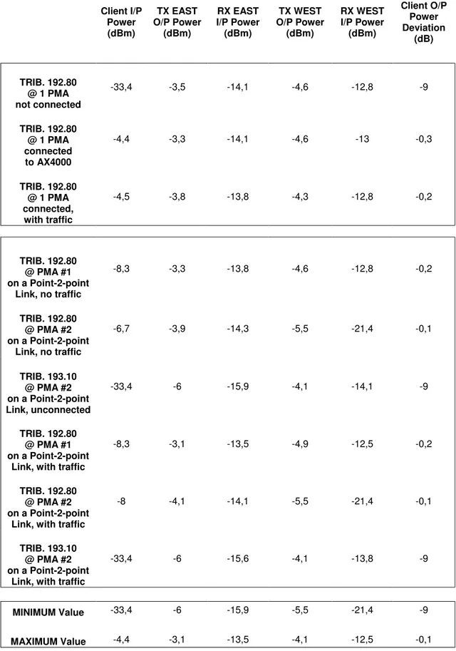
Figure 3.48 – Final Resume of the values obtained for the PMA-32’s transponders with all the tests

(31)

90

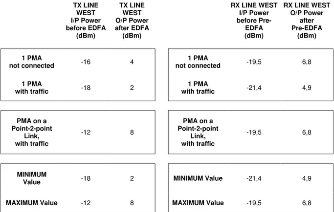
We can have a look at 2 final Figures 3.48 / 49 reporting a resume of all the tests we have used to better analyze the Analogue Monitor Display function in the management software.

Figure 3.49 – Final Resume of the values obtained for the PMA-32’s TX & RX Lines

We finally highlight that the same values of Figure 3.49 have been obtained also for the TX & RX Line East.

The data we have seen in the last experiments seem to be more or less the same as in the single PMA, and it’s presumable that the small difference in some TX section or RX section power values is due to the different interface the PMA’s see when we connect either the AX4000 or the CNIT Router-tester. Same thing for the 192.80 tributary, which seems to have the usual data with the only exception regarding the client I/P power – confirming the meaning of our interpretation.

Resuming what we have done, we can say that the Analogue Monitor Display, apart from indicating the main transmission and reception data, and the way the add/ drop functions are hardware-implemented in the system, doesn’t really show us big differences when traffic is being sent from when no traffic is getting through the PMA/PMA’s.

The only immediate data we get using this software is whether the channels are configured in a good way and if the fiber cables are connected - otherwise we would read a standard -33.4 dBm in the I/P client field. Actually we noticed that many times in the analysis above.

In the next section we’re going to concentrate more on the performance of the PMA’s considering packets delivery, which seems to be more productive at this point.

TX LINE WEST I/P Power before EDFA (dBm) TX LINE WEST O/P Power after EDFA (dBm) RX LINE WEST I/P Power before Pre-EDFA (dBm) RX LINE WEST O/P Power after Pre-EDFA (dBm) 1 PMA not connected -16 4 1 PMA not connected -19,5 6,8 1 PMA with traffic -18 2 1 PMA with traffic -21,4 4,9 PMA on a Point-2-point Link, with traffic -12 8 PMA on a Point-2-point Link, with traffic -19,5 6,8 MINIMUM

Value -18 2 MINIMUM Value -21,4 4,9

(32)

91 3.3 AX4000 as PMA-32 TESTER

3.3.1 BRIEF INTRODUCTION TO THE AX4000

In this chapter we are going to analyze some performance parameters on a single PMA and on an optical fiber topology connecting some PMA’s.

We’ll use a useful Traffic Generator & Analyzer to send and receive simulated traffic: the Spirent AX4000.

Actually we are using Gbit Ethernet optical cards, inserted in the AX interface as the one shown in the picture below.

AX Generator/Analyzer interface

The immediate impact of a user with the Spirent software is shown below: the GUI is useful to configure the testing applications in a simple Windows operative system.

AX4000 GUI – Graphical User Interface

We’ll consider in our tests both the GENERATOR features and the ANALYZER features. The main windows regarding these two components are shown in the following pictures, and the reader can immediately notice the simple approach of this software, which seems to be very user-friendly.

(33)

92

IP Generator IP Analyzer

“What can we do with the AX IP Generator” is the subject of this paragraph; we can: - create up to 8 traffic sources,

- select different priority to the given sources by using the Traffic Prioritizer, - generate errors for tests using the Error Injector feature.

Instead the IP Analyzer gives us the possibility to: - use filters at the rx interface,

- create graphical representations about statistics such as:

Packet Count, Lost Packet Count, Packet rate, % Bandwidth, Min/Max Transfer Delay,

Bit Error Count, Bad Encapsulation Count,

- generate histograms for some statistics such as the Packet Transfer Delay, that we’ll use many times for our analysis,

- capture the received packets having a complete view on the fields they contain.

Let’s also have a look at the window that lets us select the kind of traffic we want for each traffic source:

(34)

93

As for the packet sequence we can choose: The possible traffic distributions are:

-Fixed Length

-

Periodic Packet

-Uniform Distribution

-

Manually Triggered Packet

-Gaussian Distribution

-

Randomly Spaced Packet

-Quad-modal Distribution.

-

Manually Triggered Burst

as shown in the 1st picture below. -

Periodic/Randomly Spaced Burst

-

Markov Modulated Poisson Process

Packet Sequence possibilities Traffic Distribution possibilities

We’ll also select different packet lengths and various %bandwidths during our tests on the PMA-32.

To do this we can define the length in the window shown below:

Datagram Length possibilities

From a practical point of view, we have connected our AX4000 to the PMA-32 using single-mode fiber cables, and single-mode adaptation modules for the Gbit Ethernet interface.

In the following paragraphs the first approach will be with the point-to-point link between 2 PMA’s; the second one will be with particular attention to a single PMA.

(35)

94 3.3.2 SENDING TRAFFIC ON A POINT-TO-POINT LINK

BETWEEN 2 PMA-32 ’s

This experimental analysis will give us a general idea on the way our point-to-point link between two PMA’s works.

For the measures we’ll use the AX4000 Traffic Generator & Analyzer, which is useful for a simple and immediate approach to some measured network parameters.

We have connected the AX4000 to the Pma’s 192.80 tributary – so transmitting with the Generator part onto the 192.80 transponder, which connects us directly to our fiber link, and to the second PMA. In the second PMA’s 192.80 transponder we’ve configured a pass-through – so the signal we’re transmitting with the AX4000 Generator will be immediately received by the AX4000 Analyzer at the end of the ring - without being treated in other ways.

As for the kind of traffic, we’ll use some different situations to control the point-to-point link – exactly using standard packet lengths (as in Figure 3.50) and different bandwidth values on the link.

(36)

95

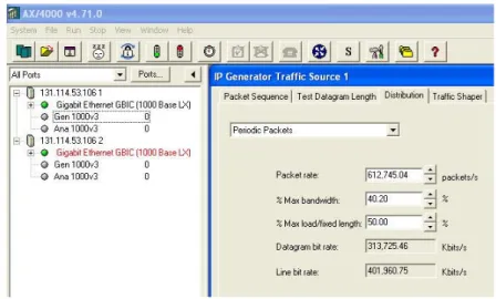
1st APPROACH:

Mode: IP test blocks Distribution: periodic packets

Fixed datagram length: 64 Max. load/fixed length: 50%

First of all we must notice that 50% of the link capability is not exactly in coincidence with 50% bandwidth (but about 40%) for level 2 Ethernet and level 3 IP overhead reasons – so the transmission is supposed to be at full saturation at 80% bandwidth.

This is noticeable in Figure 3.51.

Figure 3.51 – Selection of the desired traffic in the AX4000 Generator

In this test and in the next ones we’ll indicate in every figure the LOST PACKET COUNT in red, the MAXIMUM TRANSFER DELAY in green, and the % BANDWIDTHin blue. In Figure 3.52 there’s the result after selecting 64 byte packets with 50% Max load/fixed length.

(37)

96

2nd APPROACH:

Mode: IP test blocks Distribution: periodic packets

Figure 3.53 – 64 byte packets; 80%

3rd APPROACH: Mode: IP test blocks Distribution: periodic packets

(38)

97

Let’s have a look at the obtained Packet Transfer Delay histograms (Figures 3.55 a b c d), showing in a better way the latency of the packet before being received – which is also the #1 parameter we’re interested in.

In the cases seen until now we notice that the latency of a packet is always between 122 and 123 usecs, quite a big time interval probably due to the 72Km of fiber cables connecting the 2 PMA’s. We will understand the way the ring is influencing the latency later, analyzing the impact of a simple PMA on the packet transfer delay.

As we can see in the pictures below, the dispersion interval around the medium latency value increases when the % bandwidth gets higher.

Figure 3.55 a b c d – Packet transfer delay histograms obtained with increasing % bandwidth values

4th APPROACH: Mode: IP test blocks Distribution: periodic packets

The importance of this particular test consists of considering the 100% bandwidth – which represents the 124% of the real link occupation.

As a matter of fact we’ll notice that, as the real available traffic is the Max load/fixed length parameter’s one, even in this case the graphic will show an 80% only bandwidth, as in

(39)

98

Let’s now start sending 128 byte packets: we’re interested in understanding what changes when we send bigger packets, considering that big packets mean less overhead – Ethernet overhead and IP overhead – on the link.

5th APPROACH: Fixed datagram length: 128 Max. load/fixed length: 50%

(40)

99

6th APPROACH:

Comparing Figure 3.59with Figure 3.54 we can see that increasing the packet length the gap between % Bandwidth and % Max. load/fixed length gets smaller and smaller – as the overhead gets smaller too.

(41)

100

8th APPROACH:

As we can see we’re using 113% this time – to reach 100% bandwidth as before.

But it’s useless to try this Max. load/fixed length value on the way to have a real 100% bandwidth performance, because we’ll get the same result as in approach #7 (Figure 3.59)

Now we’re going to consider 512 as packet length. 9th APPROACH: Fixed datagram length: 512 Max. load/fixed length: 50%

(42)

101

10th APPROACH:

(43)

102

Even in the next approach we expect the bandwidth not to be changed, because we’re going to use 103% - corresponding to our 100% nominal bandwidth.

And last we’re seeing the 1500 byte packets:

13th APPROACH: Fixed datagram length: 1500

Max. load/fixed length: 50%

(44)

103

14th APPROACH:

The consideration we can underline (visible in Figures 3.67 & 3.68) is that with 1500 byte packets we can almost reach 100% bandwidth because the level 2 and 3 overheads do not take too much space on the line – so nominal bandwidth and Max. load/fixed length are more or less the same value.

(45)

104

16th APPROACH:

Another useful information we can add is about the Packet Transfer Delay histogram given by the AX4000 Analyzer. We show in the following Figures 3.69 a-b-c the histograms obtained sending 1500 byte packets, to compare them with the ones we got when analyzing the smallest packet length, which was 64 bytes.

Figures 3.69 a b c – Histograms obtained with 1500 bytes packets – 50%,80%,100% bandwidth

(46)

105

So considering different packet lengths we get a medium packet transfer delay which stands between 122 and 123 microseconds: in the later analyses we could consider a medium 122.8 microseconds.

If we want this result to be very precise for our analysis we have to measure the packet transfer delay due to the AX4000 Generator/Analyzer. We can do this not connecting the PMA to the AX and generating traffic only throughout the AX system.

Sending simulated packets with a length between 64 and 1500 bytes we usually got a medium packet transfer delay of about 0.65 usecs as shown in Figure 3.70.

Figure 3.70 - Packet Transfer Delay due to the AX4000

This result lets us consider the AX4000 as a good apparatus because it doesn’t add any particular delay to the metro-ring delay we want to verify later in this chapter.

More precise tests about the packet transfer delay considering different topologies will be shown in the MULTIPLEXING ON A POINT TO POINT LINK paragraph.

In another test we had at the CNIT block, interfacing 2 PMA’s to each other generating packets with a Router-tester we got a 2.69 usecs delay on the ring, and a 0.70 delay due to the tester, so a single PMA seemed to insert an approximate 1 usec delay.

(47)

106 3.4 SNC PROTECTION

IN THE PMA-32

In the procedures shown in the paragraph about the PMA-32 configuration we have considered the SNC PROTECTION, so we are going to face it in details, because we have to understand the way the PMA-32 works in case of signal fail.

There are two forms of traffic protection provided in the PMA-32:

-

SNC PROTECTION

-

1+1 CLIENT PORT PROTECTION

3.4.1 SNC PROTECTION MECHANISM

The PMA-32 Sub-network Connection Protection (SNCP) mechanism is designed to protect against equipment failure within a PMA-32 network. Equipments such as

SDH/SONET elements will continue to use their own protection schemes with the PMA-32 providing the number of fibers required by those elements.

There are two forms of SNC protection provided in the PMA-32: - INTRA CARD 1+1 SNC PROTECTION

- INTER CARD 1+1 SNC PROTECTION

Let’s talk about the first one, which is the protection type we are more interested in. The same considerations will be useful for the Inter-card protection.

INTRA CARD 1+1 SNC PROTECTION

This form of protection for optical channels within a WDM ring is achieved by means of provisioning Protected Transponder/Tributary Units.

These units effectively split the incoming optical client signal into two identical signals that are subsequently presented to the west and east add/drop units respectively...

Hence the client traffic signal is sent in both directions around the ring, thus providing a diverse route for each client signal through the optical network.

On the Protected Transponder/Tributary Unit in the receive direction, two signals (one from each of the add/drop units) are presented to a selector. The selector chooses the relevant receive channel according to optical channel signal failure conditions or operator commands.

Once activated the Intra Card SNCP, as explained in the section named “HOW TO CREATE A CROSS-CONNECTION USING THE MANAGEMENT SOFTWARE” available in the PMA CONFIGURATION paragraph, one can change some parameters as we are going to explain in the following lines.

We can first of all open the “Amend SNC Protection” window (Figure 3.71), which contains all the configurable modes and commands regarding the working and protection lines.

(48)

107

Figure 3.71 – Amend SNC Protection window

WORKER / PROTECTION / PROTECTION STATE

The “Worker” and “Protection” shown in the picture above are the lines in use at the moment of consulting the Amend Protection window – using for example the “Swap worker/protection” command the indication will change.

Besides the “Protection State” lets us know where the traffic is being sent.

This is going to be very useful for the experimental experiences we have to face in this paragraph, because we can always analyze the link situation using this window.

PROTECTION LOCKOUT

This command causes the traffic to be maintained on the current (worker or protection) channel. This command has a higher priority than locally detected failures and operator switch commands, hence traffic remains on the current channel regardless of any failure indications on this channel.

PROTECTION MODES

There are four modes of operation all of which are operator-configurable: - Dual ended – Revertive

- Dual ended – Non – Revertive - Single ended – Revertive - Single ended – Non – Revertive

Single Ended – Revertive Mode

(49)

108

The preferred channel is denoted as the ‘worker channel’ and the channel used for

protection purposes is denoted as the ‘protection channel’.

- When there are no failure conditions or active operator entered commands, the receive selector selects traffic from the designated worker channel.

- If there is a failure on the worker channel the switching mechanism, under normal circumstances, automatically causes a changeover to select traffic from the protection channel.

Upon recovery of the worker channel, the selector is automatically switched to select this channel in preference to the protection channel (after the expiry of a ‘Wait to Restore’ period).

Single Ended – Non Revertive Mode

This mode of operation is identical to revertive mode except that traffic is not switched back to the worker channel from the protection channel when the former recovers from a failure condition or an operator command is cleared. This prevents the disturbance to traffic which would otherwise occur when the selector is operated.

However, the two channels are still designated ‘worker’ and ‘protection’.

The PMA–32 selects traffic from the designated ‘worker’ channel as a default when first configured for SNC protection or on power-up of the PMA-32.

Dual Ended – Revertive Mode

In this mode traffic is switched automatically to the same (worker or protection) channel at each end of the path. Bits within the Optical Channel _ OH are used to ensure that the PMA’s at each end of the path always switch to the same channel.

In revertive mode (Dual Ended) there is a preferred channel for receiving the optical channel.

The preferred channel is denoted as the ‘worker channel’ and the channel used for protection purposes is denoted as the ‘protection channel’.

As above, when there are no failure conditions or active operator entered commands, the receive selector selects traffic from the designated worker channel. If there is a failure on the worker channel the switching mechanism, under normal circumstances, automatically causes a changeover to select traffic from the protection channel. The bits within the Optical Channel _OH are then used to ensure that the selector at the far end of the path also automatically selects its protection channel.

Upon recovery of the worker channel, the selector is automatically switched to select this channel in preference to the protection channel (after the expiry of a ‘Wait to Restore’ period).

The bits within the Optical Channel _ OH are this time used to ensure that the selector at the far end of the path also automatically selects its worker channel.

Dual Ended – Non Revertive Mode

As in the Revertive Mode (Dual Ended) above, traffic is switched automatically to the same (worker or protection) channel at each end of the path.

Traffic shall not be switched back to the worker channel from the protection channel when the former recovers from a failure condition or an operator command is cleared.

This prevents the disturbance to traffic, which would otherwise occur when the selector is operated, as we already said for the Single Ended case.

(50)

109

Mode Mismatch

When operating in dual ended mode normally both the local and remote ends of the path are configured for the same mode.

In the event that each end is configured differently a ‘mode mismatch’ alarm is raised and the local operating mode is autonomously reconfigured to a single ended mode. The ‘mode mismatch’ alarm is autonomously disabled if the protection channel has failed. The operator is warned that a ‘mode mismatch’ alarm from one end of the channel only is indicative of failures at both ends of a protected channel defeating the dual ended control mechanism.

“WAIT TO RESTORE” OR “DO NOT REVERT”

The PMA–32 enters either ‘Wait to Restore’ or ‘Do Not Revert’ state when the worker channel recovers from a failure.

“Wait To Restore” State

The ‘Wait to Restore’ is entered automatically when traffic is selected from the protection channel (due to a failure of the worker channel) and the worker channel subsequently recovers (revertive mode only).

Entry to the ‘Wait to Restore’ state is inhibited if a higher priority condition exists when the worker channel recovers.

When the ‘Wait to Restore’ state is entered, a timer is set and the condition is deactivated upon expiry of the timer period.

The timer is operator configurable.

Selection of the 0 minute option prevents a protected channel from ever entering the ‘Wait to Restore’ condition (i.e. it will deselect the ‘Wait to Restore’ option). “Do Not Revert” State

The ‘Do not Revert’ state is entered under the same circumstances as ‘Wait to Restore’ except that there is no timer and it remains active until a higher priority condition is received.

‘Do not Revert’ is used in non–revertive mode of operation only.

OPERATOR COMMANDS

The following commands are available for operator control of the traffic selector:

-

Force switch to protection

-

Force switch to worker

-

Manual switch to protection

-

Manual switch to worker

-

Clear

Force Switch To Protection

This command causes traffic to switch to (or be maintained on) the designated protection channel. The command has a higher priority than locally detected failures on the

protection channel and hence traffic remains on the protection channel regardless of any failure indications on this channel.

Force Switch To Worker

This command causes traffic to switch to (or be maintained on) the designated worker channel. This command has a higher priority than locally detected failures on the worker channel and hence traffic remains on the worker channel regardless of any failure indications on this channel.

(51)

110

Manual Switch To Protection

This condition causes traffic to switch to (or be maintained on) the protection channel unless a higher priority switch command is in effect. Note that the manual switch

command has a lower priority than locally detected conditions on the protection channel. Manual Switch To Worker

This command causes traffic to switch to, or be maintained on the designated worker channel unless a higher priority switch state is in effect. Note, in particular, that detected conditions on the worker channel have a higher priority than the manual switch command. Clear

This command clears any operator entered command (except Swap Worker/Protection Designation).

SWAP WORKER/PROTECTION DESIGNATION

This command changes over the current channel designations, for example the west going connection from ‘worker’ to ‘protection’ and the east going connection from ‘protection’

to ‘worker’.

PROTECTION HOLD OFF TIME

If SNCP is used at the same time as other protection schemes operating externally to the PMA, then there may be a need to ensure that the SNCP switches a certain period (Hold Off Time) after the ‘other’ scheme.

A protection status event is not reported until the ‘Hold Off’ timer has expired and hence the selector has operated.

The ‘Hold Off’ timer value is operator configurable.

SIGNAL FAIL / SD DETECTION

Autonomous control of the traffic selector is by means of signal optical channel quality criteria represented by two internally generated flags:

-

Signal Fail (SF)

-

Signal Degrade (SD)

A Signal failure (SF) indication shall be raised if one, or more, of the following criteria are detected:

-

Rx Optical Channel Loss of Signal

-

Rx Optical Channel Loss of Frame

-

Rx Optical Channel Excessive BER

-

Rx Optical Channel Regenerator Loss of Signal

-

Rx Optical Channel FDI

-

Rx Optical Channel Payload Type Identifier Mismatch

-

Rx Optical Channel Payload Type Identifier Unequipped

-

Rx Optical Channel Trace Identifier Mismatch

A Signal Degrade (SD) indication shall be raised if the following condition is detected:

-

Rx Optical Channel Degrade, or Rx Optical Channel Degraded BER, or Disabled.

3.4.2 EXPERIMENTS ON A RING INVOLVING 2 PMA’s

What we need to verify in this section is what happens if a SIGNAL FAIL is detected – and we can simulate this situation un-connecting the TX/RX West/East fiber cables in the core of a PMA situated on the link.

(52)

111

The configuration we’ll use is 2 of the 3 PMA’s we have at the CNIT block (A3 & A2) connected on a ring – which becomes a point-to-point link.

Let’s see the tributaries we have at each PMA-32 (Figures 3.72 & 3.73):

Figure 3.72 – A3 PMA equipment

Figure 3.73 – A2 PMA equipment

In both figures we have highlighted the 193.10 frequency, which is the one we’ll use for this test.

(53)

112

As we can notice in the pictures Intra Card protection has been chosen for both

transponders.

Besides in both PMA’s we see in the above pictures that the 193.10 tributary’s working channel has been configured on the West TX line.

We immediately verify that we can also change this local indication by deleting the cross-connections and creating new ones choosing the East TX line – but the easiest way to do this is through the SWAP WORKER / PROTECTION option.

With this feature, we’ll see EAST instead of West. We have done that only on the A3 PMA, so in the following tests we are going to analyze the system with the A3 Worker starting at the TX East and getting back to the RX East, and the A2 Worker starting at the TX West and getting back to the RX West. So the protection lines will start and stop at the West part of the 1st PMA, and at the East terminal of the 2nd PMA – but we’ll notice more about the topology a little later, when using the Amend SNC protection which is a kind of reminder on the way the ring has been created.

TEST #0 (START LEVEL): RING with NO SIGNAL FAIL

Let’s start by viewing the standard situation when no problem is detected, that is to say we haven’t un-connected any fiber cables on the double ring.

To test the ring we’re using a Router-tester which sends traffic onto the A3 PMA.

The ports we use (shown in Figure 3.74) named as 101.1 and 101.2 have this role in this experiment:

- 99% of 1Gbit is sent from port 101.1 to port 101.2 - that is to say this simulated traffic enters the A3 PMA, hence going through the ring.

- 10% of 1Gbit is sent from port 101.2 to port 101.1 – so this traffic enters the ring through the A2 PMA, our second PMA apparatus.

(54)

113

The Router-Tester picture shown above lets us analyze the TX and RX test packets, the latency and other parameters.

We’ll concentrate on the latency, and on the way the system works when a fail hits the ring, thus forcing the PMA to send traffic on the protection line.

We’ll have in test 0 the following situation in the Amend SNCP window (Figure 3.75):

Figure 3.75 - Amend SNC Protection window when the worker channel is LINE EAST

First of all we notice that the worker is LINE EAST (meaning TX EAST) and the protection is LINE WEST (meaning TX WEST). The protection state field signals that traffic is on worker, so no problem is detected on the link.

Revertive mode has been selected – this means that if there should be a signal fail on the link, if the working line were up again the signal would be immediately resent on the worker.

The protection mode is now seen as SINGLE ENDED – that is to say if there should be failures on a PMA, on the others there wouldn’t be any changes . We’ll explain better this option in the next paragraph.

There’s no lockout that may disturb the process of changing the worker with the protection in case of signal fail.

Finally operator command is “Clear”, that is to say there’s no operator’s forcing switch. “NO REQUEST, TRAFFIC ON WORKER” shows that the link is currently working with no signal fail message.

All the following tests will be done on the A3 PMA.

TEST #1: SIGNAL FAIL on TX WEST

As we know the traffic is being sent on the EAST LINE Worker, with West protection (Figure 3.76).

The simulation is about a fail on the TX WEST terminal.

What we get in the picture above is first of all the Protection State field marked with “SIGNAL FAIL ON PROTECTION – TRAFFIC ON WORKER” – thus meaning that the signal is still being sent on the Worker (that is to say line EAST), while we have simulated a problem on the protection line (west) – actually we have just done that, because we unconnected the West TX fiber cable.

(55)

114

Figure 3.76 – Amend SNC protection window in case of fail on TX WEST

The only thing we have to clarify is that, as we are working on a point-to-point link between two PMA-32’s with a router-tester, even if the physical topology of the ring doesn’t change as for the fiber cables, the logical topology has changed.

In fact in the following tests we’re going to verify that the chosen “Worker” starts from the TX EAST line and comes back to RX EAST terminal, but we’re getting this later.

TEST #2: SIGNAL FAIL on RX EAST

In this case we are attempting to simulate a case of fail on the RX EAST terminal. It creates a “SIGNAL FAIL ON WORKER – TRAFFIC ON PROTECTION” in the

Protection state field, meaning that we have a problem on the working line (actually it has been designated as the East one) and that the protection line is being used for the traffic we cannot send on the main line at the moment (Figure 3.77).

(56)

115

This means that the PMA-32 is working properly letting us use the protection line exactly in the way it has been projected for.

We have the means now to understand better the logical topology of this point-to-point link, which is useful for our analysis. In a topology like this, with the Worker of a PMA on the opposite direction of the Worker on the other PMA, we have the signal going out of the 1st PMA through TX West or East and getting back after the point-to-point link through RX West or East respectively; in our case we get out of the PMA using the TX east and we get back to it using RX east. This freedom to create the topology may create confusion when analyzing a system having more than 2 PMA’s, but it also gives good potentialities to reduce the latency and to decide what paths to select.

Let’s include in the explanation - always talking about the RX EAST signal fail – the case when a NON-Revertive mode has been chosen in the Amend SNC protection preferences. What happens in this case? The protection state will be “Do not revert” and if the fail

should be solved and the RX East reconnected we would not have the traffic back on the line designated as Worker.

Figure 3.78 – No more fail on RX East – NON REVERTIVE mode

(57)

116 TEST #3: SIGNAL FAIL on TX EAST

In this case we have a simulated fail on the TX East unit – we expect it to be another test with the same result as in the RX EAST fail.

Actually Figure 3.80 shows us what we supposed, because “SIGNAL FAIL ON WORKER – TRAFFIC ON PROTECTION” appears in the protection state field – and the traffic is redirected to the protection line, being the Worker out of order.

TX East is just the start part of the east ring, marked as worker, and closing the fiber link on the RX East terminal.

Figure 3.80 - Amend SNC protection window in case of fail on TX East

With the revertive mode flag we are sure that after reconnecting the TX East cable we’ll get in something like 20 seconds or a little more, depending on the processing time due to the PMA-32, a new indication in the protection state: “No Request – Traffic on Worker” as in Figure 3.75.

TEST #4: SIGNAL FAIL on RX WEST

Finally we get “SIGNAL FAIL ON PROTECTION – TRAFFIC ON WORKER” in the RX West failing case (Figure 3.81), so we understand that even in this case, as in the TX WEST one, the protection is not working correctly, so if there were problems on the working line we would not have an alternative path to redirect the traffic to.

After solving the fail, we should have the same indication as in the protection state we see in Figure 3.75.

TEST #5: WORKER-PROTECTION SWAPPING

An interesting potentiality of the PMA-32 is the “Swap Worker/Protection function”, which is useful for example in this case, because we want to see what happens if we redirect the Worker channel traffic onto the protection line, doing the same thing with the protection line traffic.

(58)

117

Figure 3.81 - Amend SNC protection window in case of fail on RX West

The SWAP function is surely easier than trying to manually configure the single transponder cards,as we said at the beginning of this section. Besides we can decide what tributaries to swap and what to leave with the present Worker/Protection

configuration.

In Figure 3.82 we show how to activate the Swap option.

(59)

118 TEST #6: WRONG CONFIGURATION: Pass-through on the A2 PMA

This case seems to be very useful to understand better and better the way the SNC protection works: let’s not change the A3 PMA configuration, while we’re activating a pass-through on the A2 PMA for the 193.10 frequency, thus leaving the signal unchanged when passing through the second PMA.

Not facing an add or drop action at the A2 PMA the protection we have configured at the A3 PMA doesn’t seem to have any correspondence at the other end of the ring.

The latency we measure is 3,36 useconds.

Trying to test the possible signal fail, un-connecting the Worker, we’ll notice that the bandwidth goes down to 0% because there’s no clear configuration for the protection ring (Figure 3.83).

Figure 3.83 – Router-tester analysis when simulating a signal fail on the ring

When trying to reconnect the ring, the signal fail disappears and the bandwidth has the right value again – thus letting the router-tester show the latency values, which haven’t been indicated during the signal fail indication.

(60)

119

Figure 3.84 - Router-tester analysis during the transition between signal fail and ring working again

The conclusion we can add here is that a link like this is not interesting for our analysis, because the SNC protection will not work properly.

Actually in Figure 3.85 we can see the indication “SIGNAL FAIL ON PROTECTION” in the Amend SNC Protection window.