Lecture notes in quantitative methods for economists

(1)

Lecture notes in quantitative methods for economists:

Statistics module

Appunti per il corso di Metodi Quantitativi per Economisti, modulo di Statistica

Antonio D’Ambrosio

Draft 1

Napoli, Ottobre 2020

(2)

(3)

Preface

Questi appunti raccolgono gli argomenti che vengono trattati al corso di Metodi Quantitativi per Economisti nell’ambito del corso di Laurea Magis- trale in Economia e Commercio dell’Universit`a degli Studi di Napoli Federico II.

Non si pretende di fornire agli studenti un materiale migliore rispetto ai tanti eccellenti manuali presenti in letteratura, molti dei quali sono consigliati per lo studio di questo insegnamento. Si esortano anzi gli studenti a far riferi- mento alle fonti consigliate durante il loro percorso di studio. Il proposito `e piuttosto quello di fornire un indice degli argomenti trattati durante il corso, riunirli tutti in un unico corpus e fornire una breve (e non esauriente) guida alla riproduzione degli esempi riportati attraverso il software R.

Questi appunti sono stati volutamente scritti in lingua inglese per una serie di motivi:

la letteratura sul tema `e quasi interamente disponibile in lingua inglese;

gli studenti frequentanti un corso di laurea magistrale devono essere in grado di studiare e approfondire i temi studiati da fonti in lingua inglese;

in virtú della crescente internazionalizzazione delle Università, è sempre più frequente avere in aula studenti stranieri, magari frequentanti il programma Erasmus.

Gli argomenti trattati riguardano il modello di regressione lineare ed una introduzione all’analisi della varianza. Un programma del modulo statistico dell’insegnameto di Metodi Quantitativi per Economisti tarato in questo modo dovrebbe preparare gli studenti allo studio di altre discipline quantitative in ambito sia economico che statistico, quali ad esempio econometria, modelli lineari generalizzati, data mining, analisi multivariata, categorical data analysis, ecc.

Si suppone che gli studenti abbiano frequentato sia un corso di Statistica nel quale si siano affrontati i temi principali dell’inferenza statistica ed una

III

(4)

una introduzione all’algebra delle matrici.

Questi appunti sono dinamici: potranno cambiare di anno in anno, potranno includere nuovi argomenti, potranno escluderne taluni. La loro struttura si modificher`a a seconda delle esigenze didattiche del corso di Lurea, ma soprat- tutto seguendo i commenti degli studenti dai quali mi aspetto, se lo vorranno, consigli e critiche costruttive su come modificare e migliorare l’esposizione degli argomenti proposti.

Anche se l’impostazione di questi appunti `a prevalentemente teorica, sono riportati diversi esempi riproducibili in ambienteR attraverso una operazione di ”copia-e-incolla” delle funzioni utilizzate. Si precisa per`o che lo scopo non

`e quello di imparare ad usare un linguaggio di programmazione: per questo vi sono insegnamenti appositi. Laddove non specificato espressamente, i data set utilizzati, tutti con estensione.rda(l’estensione dei dati di R) sono scar- icabili dal sito http://wpage.unina.it/antdambr/data/MPQE/.

Queste pagine contengono sicuramente errori e imprecisioni: sar`o infinita- mente grato a chi vorr`a segnalarli.

(5)

Chapter 1

Regression model: introduction and assumptions

1.1 Regression analysis: introduction, definitions and notations

Regression analysis is used for explaining or modeling the relationship between a single variableY, called theresponse variable, oroutput variable, or dependent variable, and one or more predictor variables, or input variables, orindependent variables orexplanatory variables, X₁, . . . ,X_p.

The data matrix is assumed to be derived from a random sample ofn observations (xi1, xi2, . . . , xip, yi), i= 1, . . . , nor, equivalently, an n×(p+ 1) data matrix.

When p = 1, the model is called simple regression; when p > 1 the model is called multiple regression or sometimes multivariate regression. It can be the case then there are more than one Y: in this case the model is called multivariate multiple regression.

The response variable must be continuous as well as the explanatory variables can be continuous, discrete or categorical. It is possible to extend the linear regression model to response categorical variables through the Generalized Linear Models (GLM): probably you will study GLM in the future.

Let’s define some notations and definitions.

Letn be the sample size;

Letp denote the number of predictors;

LetY = (Y₁, Y₂, . . . , Y_n)^T be the vector of the dependent variables.

(10)

Let y= (y₁, y₂, . . . , y_n)^T be the vector of the sample extractions from Y.

LetX be the n×(p+ 1) matrix of the predictors.

Let= (₁,₂, . . . ,_n)^T be the vector of the error random variables_i.

Let e = (e₁, e₂, . . . , e_n)^T be the vector of the sample extractions from .

Letβbe the vector of the (p+1) parameters to be estimatedβ₀, β₁, . . . , β_p. The linear regression model is

Y =Xβ+, or, equivalently,

Y =β0+β1x1 +. . .+βpxp +.

1.2 Assumptions of the linear model

The relationship betweenY and the (p+ 1) variables is assumed to be linear.

This relationship cannot be modified because the parameters are assumed fixed. The linear model is:

Yi =β0+β1xi1+β2xi2+. . .+βpxip+i

in which the _i, i = 1, . . . , n are values of the error random variable , mutually independent and identically distributed, E(_i) = 0, var(_i) = σ². In other words, the error random variable has null expectation and has constant variance (homoscedasticity).

The distribution ofis independent of the joint distribution ofX₁, X₂, . . . , X_p, from which it follows thatE[Y|X1, X2, . . . , Xp] =β0+β1X1+β2X2+. . .+βpXp

and var[Y|X₁, X₂, . . . , X_p] =σ².

Finally, the unknown parameters β₀, β₁, , . . . , β_p are constants. The model is linear in the parameters, the predictors do not have to be linear.

Of course, in real problems we deal with sample observations. Once the random sample has been extracted, we have the observed values y sampled fromY. Hence, on the observed sample, we have

y=Xβ+e,

(11)

1.2. Assumptions of the linear model

in which the vectorecontains the sample extractions from. Note that if we know theβ parameters, thane is perfectly identifiable becausee =y−Xβ.

The regression equation in matrix notation is written as:

y=Xβ+e (1.1)

yn×1 =





 y₁ y₂ ... y_n







Xn×(p+1) =







1 x₁₁ . . . x_1,p 1 x₂₁ . . . x_2,p ... ... ... ... 1 x_n1 . . . x_n,p







β_(p+1)×1 =





 β₀ β₁ ... β_p







en×1 =





 e₁ e₂ ... e_n







The X matrix incorporates a column of ones to include the intercept term (now it should be clear the meaning of the notation in which the predictors are said to be p+ 1: p predictors + the intercept). Let’s see the (classical) assumption of the regression model.

Assumption 1: linearity

Linear regression requires the relationship between the independent and dependent variables to be linear. It means that this assumption imposes that

Y=Xβ+ .

Assumption 2: the expectation of the random error term is equal to zero

E[] =





 E[₁]

... E[_n]





=





 0

... 0





.

This assumption implies that E[Y] =Xβ because

E[Y] =E[Xβ+] =E[Xβ] +E[] =Xβ.

The average values of the random variables that generate the observed values of the dependent variable ylie along the regression hyperplane.

3

(12)

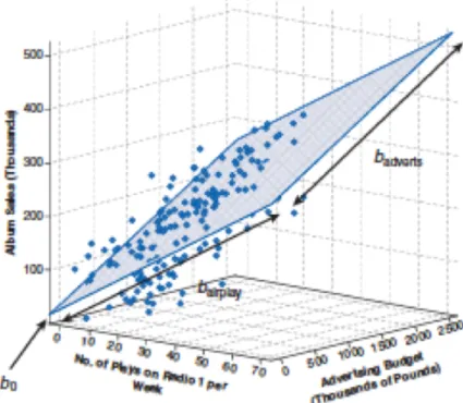
Figure 1.1: Regression hyperplane. the response variable (Album sales) is represented on the vertical axis. On the horizonal axes are represented the two predictors: Advertising budget and Airplay. The dots are the observed values. The regression hyperplane is highlighted in gray with blue countour

Assumption 3: Homoscedasticity and incorrelation between random terms

The variance of each error term is constant and it is equal toσ², furthermore cov(_i,_j) = 0 ∀i6=j.

var[] =E[^T] =σ²I, namely

(13)

1.2. Assumptions of the linear model

var[] = E[^T]−E[]E[^T]

= E[^T]

=







E[₁₁] E[₁₂] . . . E[₁_n] E[21] E[22] . . . E[2n]

... ... . .. ... E[_n₁] E[_n₂] . . . E[_n_n]







=







σ² 0 . . . 0 0 σ² . . . 0 ... ... . .. ...

0 0 . . . σ²





 .

Assumption 4: no information from X can help to understand the nature of

When we say that the nature of the error term cannot be explained by the knowledge of the predictors, we assume that

E[|X] =0

Assumption 5: the X matrix is deterministic, not stochastic Assumption 6: the rank of the X matrix is equal to p+ 1

By saying the X must be a full-rank matrix, it is clear that the sample size n must be less of equal to p+ 1. Moreover, the independent variables X_j, j = 1, . . . , p are supposed to be linearly independent, hence they cannot be expressed as a linear combination of the others. If the linearly indepen- dence of the predictors is not assumed the model is not identifiable.

Assumption 7: the elements of the (p+ 1)1 vector β and the scalar σ are fixed unknown numbers with σ > 0

Suppose to deal with a random sample, starting from the observed y and X the goal is to obtain the estimate βˆof β. The model to be estimated is

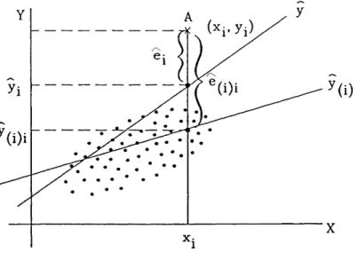
yi =Xiβˆ+ ˆei, i= 1, . . . , n ,

where ˆe_i = y_i −yˆ_i is called residual, with ˆy_i = X_iβ. We can resume theˆ expressed concepts in this way (Piccolo, 2010, chapter XXIII).

5

(14)

Y =Xβ+ ⇒ =Y−Xβ Teoretical model

y=Xβ+e ⇒ e=y−Xβ General model

ˆ

y=X ˆβ ⇒ eˆ=y−X ˆβ Estimated model

Remember: the vectorcontains the error random variablesi; the vector e, given any arbitrary vectorβ, contains the realizations of the random variables _i; the vector eˆcontains the residuals of the model after the estimate of β, that is denoted with β.ˆ

(15)

Chapter 2

Model parameters estimate

2.1 Parameters estimate: ordinary least squares

Lety=Xβ+e be the model. The parameter to be estimated is the vector of the regression coefficients

β =β₀, β₁, . . . , β_p.

Least squares procedure determines the βvector in such a way that the sum of squared errors are minimized:

n

X

i=1

e²_i =

n

X

i=1

(y_i−β₀−β₁x_1i− · · · −β_px_pi)

=

n

X

i=1

(y_i−X_iβ)²

= e^Te

= (y−Xβ)^T(y−Xβ)

We look for β for which f(β) = (y−Xβ)^T (y−Xβ) =min. Let’s expand this product:

f(β) = y^Ty−β^TX^Ty−y^TXβ+β^TX^TXβ

= y^Ty−2β^TX^Ty+β^TX^TXβ

The function β has scalar values, being β a column vector of length p+ 1.

The terms β^TX^Ty and y^TXβ are equal (two equal scalars), then they can

(16)

be summarized with 2β^TX^Ty. The term β^TX^TXβ is a quadratic form in the elements of β. Differentiating with respect to f(β) we have

δf(β)

δβ =−2X^Ty+ 2X^TXβ, and setting to zero

−2X^Ty+ 2X^TXβ= 0,

we obtain as a solution a vectorβˆ such that we obtain the so-called normal equations:

X^TXβˆ =X^Ty.

Let’s give a look to the normal equations. We have

X^TX=







n Pn

i=1x_i1 Pn

i=1x_i2 · · · Pn i=1x_ip Pn

i=1x_i1 Pn

i=1x²_i1 Pn

i=1x_i1x_i2 · · · Pn

i=1x_i1x_ip Pn

i=1x_i2 Pn

i=1x_i1x_i2 Pn

i=1x²_i2 · · · Pn

i=1x_i2x_ip

... ... ... ... ...

Pn

i=1x_ip Pn

i=1x_i1x_ip Pn

i=1x_i2x_ip · · · Pn i=1x²_ip





 .

As it can be seen, X^TX is a (p+ 1)×(p+ 1) symmetric matrix, sometimes calledsum of squares and cross-product matrix. The diagonal elements contain the sum of squares of the elements in each column ofX. The off-diagonal elements contain the cross products between the columns ofX.

The vectorX^Tyis formed by these elements:

X^Ty=





 Pn

i=1y_i Pn

i=1x_i1y_i Pn

i=1x_i2y_i ... Pn

i=1x_ipy_i





 .

Thejth element ofX^Ty contains the product of the vectorsx_j andy, hence the vector X^Ty is a vector of length p+ 1 containing the p+ 1 products between the matrix X and the vector y.

Provided that theX^TX matrix is invertible, the least squares estimate of β is

(17)

2.2. Properties of OLS estimates

βˆ= (X^TX)⁻¹X^Ty.

Of course, the solution βˆdepends on the observed values y, which are ran- domly drawn samples from the random variable Y. Suppose to extract all the possible samples of size n from Y: as the random sample varies, the estimates βˆvary too, being extractions of the Least Squares Estimator B:

B = (X^TX)⁻¹X^TY.

2.2 Properties of OLS estimates

If the assumptions of the linear regression models are verified, the OLS (Or- dinary Least Squares) estimator is said to be a BLUE estimator (BestLinear UnbiasedEstimator). In other words, within the class of all the unbiased linear estimators, the OLS returns the estimator with minimum variance (best).

This statement is formally proved with the Gauss-Markov theorem.

2.2.1 Gauss-Markov theorem

The estimator is linear.

The estimator B can be expressed in a different way:

B = (X^TX)⁻¹X^TY

= (X^TX)⁻¹X^T(Xβ+)

= (X^TX)⁻¹X^TXβ+ (X^TX)⁻¹X^T

= β+ (X^TX)⁻¹X^T

= β+A

= AY,

whereA= (X^TX)⁻¹X^T andAA^T = (X^TX)⁻¹. The estimator is linear becauseB =AY, then it is linear combinations of the random variable Y.

The estimator is unbiased.

The assumption 1 (linearity) implies thatB can be expressed asβ+A (see the point above). Then from assumptions 2 (Average of errors equal to zero), 4 (deterministic X) and 6 (Constant parameters) it follows that

E(B) =β+ (X^TX)⁻¹X^T E() =β 9

(18)

The estimator is the best within the class of linear and unbiased estimators.

The first thing to do is determine the variance ofB. From assumption 3 (Homoscedasticity) we know that E(^T) =σ²I. Hence (by recalling that we can express B=β+ (X^TX)⁻¹X^T)

var(B) = E[(βˆ−β)(βˆ−β)^T]

= E[((X^TX)⁻¹X^T)((X^TX)⁻¹X^T)^T]

= E[(X^TX)⁻¹X^T^TX(X^TX)⁻¹]

= (X^TX)⁻¹X^T E[^T]X(X^TX)⁻¹

= (X^TX)⁻¹X^T(σ²I)X(X^TX)⁻¹

= (σ²I)(X^TX)⁻¹X^TX(X^TX)⁻¹

= σ²(X^TX)⁻¹

Result 1: var(B) = σ²(X^TX)⁻¹.

Suppose that B_o is another linear unbiased estimator for β. As it is a linear estimator, we callCa generic ((p+1)×n) matrix that substitutes A= (X^TX)⁻¹X^T. We defineB_o =CY.

It is assumed that the estimator B_o must be unbiased. By recalling that (first assumption)Y =Xβ+, it must be that

E[Bo] =E[CY] =E[CXβ+C] =β,

which is true if and only ifCX=I.

Let’s introduce the matrix D = C−(X^TX)⁻¹X^T. It allows first to express C=D+ (X^TX)⁻¹X^T, and then to see that

DY=CY−(X^TX)⁻¹X^TY =β_o−β. It immediately follows that

(19)

2.3. Illustrative example, part 1

var(B_o) =σ²

(D+ (X^TX)⁻¹X^T)(D+ (X^TX)⁻¹X^T)^T

=σ²[DD^T +DX(X^TX)⁻¹ + + (X^TX)⁻¹X^TD^T + + (X^TX)⁻¹X^TX(X^TX)⁻¹]

=σ²

(X^TX)⁻¹+DD^T

= var(B) +σ²(DD^T)

Result 2: var(B_o) = var(B) +σ²(DD^T).

By combining the previous results 1 and 2, it can be seen that var(B_o)−var(B) = σ²(DD^T),

which is positive semidefinite matrix (i.e., it has non-negative values on the main diagonal).

It is clear that σ²(DD^T) = 0 if and only if D = 0. It happens only when C= (X^TX)⁻¹X^T producing B_o ≡B.

The conclusion is that, under the assumptions of the linear regression model, the OLS estimator B gives the minimal variance in the class of unbiased and linear estimators. In a few words, the OLS estimator is a BLUE estimator.

2.3 Illustrative example, part 1

2.3.1 A toy example

Computations by hand

As illustrative example, consider first a toy example in which the computations can be made (if you want) by hand. Suppose to have the following data:

11

(20)

y=





 64.05 61.64 68.43 75.85 86.77 51.03 77.38 52.27 51.12 84.13







; X=







16.11 7 14.72 3 16.02 4 15.05 4 16.58 4 15.22 8 13.95 3 14.71 9 15.48 9 13.78 3





 .

We have n = 10, p = 2. The first to do is add a column of one to the X matrix, obtaining

X=







1 16.11 7 1 14.72 3 1 16.02 4 1 15.05 4 1 16.58 4 1 15.22 8 1 13.95 3 1 14.71 9 1 15.48 9 1 13.78 3





 .

Let’s compute the X^TX matrix:

X^TX =





10.00 151.62 54.00 151.62 2306.31 824.17 54.00 824.17 350.00



.

By calling the columns of X const, X₁ and X₂ respectively, we can see that on the diagonal we have exactlyP10

i=1const²_i =n = 10, P10

i=1X_i1² = 2306.31 and P10

i=1X_2i² = 350.00.

On the off-diagonal elements we have the cross-products P10

i=1const_iX_1i = 151.62, P10

i=1constiX2i = 54.00 and P10

i=1X1iX2i = 824.17 (check by your- self).

The determinant of X^TX is equal to 4086.68, the cofactor matrix is

(X^TX)^c=





127946.15 −8560.97 418.94

−8560.97 584.00 −54.36 418.94 −54.36 75.04



, yielding to

(21)

2.4. Sum of squares

(X^TX)⁻¹ =





31.31 −2.09 0.10

−2.09 0.14 −0.01 0.10 −0.01 0.02



.

Now we have to compute the (3×1) vector X^Ty:

X^Ty=





672.67 10191.13 3380.77



.

The regression coefficients are computed in this way:

βˆ=





31.31 −2.09 0.10

−2.09 0.14 −0.01 0.10 −0.01 0.02



×





672.67 10191.13 3380.77



=





57.76 2.24

−4.52





In summary, we have ˆβ₀ = 57.76, ˆβ₁ = 2.24 and ˆβ₂ =−4.52.

2.4 Sum of squares

The results obtained with the least squares allow to separate the vector of observations y in two parts, the fitted values ˆy=Xβˆ and the residualsˆe:

y=Xβˆ+ˆe= ˆy+ˆe Since ˆβ = (X^TX)⁻¹X^Ty, it follows that:

ˆ

y = X ˆβ

= X(X^TX)⁻¹X^Ty

= Hy

The matrix H =X(X^TX)⁻¹X^T is symmetric (H= H^T), idempotent (H× H = H² = H) and is called hat matrix, since it ”puts the hat on the y”, namely provides the vector of the fitted values in the regression of yon X.

The residuals from the fitted models are

ˆe=y−ˆy=y−X ˆβ = (I−H)y.

13

(22)

The sum of squared residuals can be written as ˆe^Tˆe=

n

X

i=1

(y_i−yˆ_i)² = (y−ˆy)^T(y−y)ˆ

= (y−X ˆβ)^T(y−X ˆβ)

= (y^Ty−y^TX ˆβ−βˆ^TX^Ty+βˆ^TX^TX ˆβ)

= (y^Ty−βˆ^TX^Ty)

=y^T(I−H)y

This quantity is called theerror or (residual)sum of squares and is denoted by SSE.

The total sum of squares is equal to

n

X

i=1

(y_i−y)¯ ² =y^Ty−ny¯²

The total sum of squares, denoted by SST, it indicates the total variation in ythat is to be explained by X.

The regression sum of squares is defined as

n

X

i=1

(ˆy_i−y)¯ ² =βˆ^TX^Ty−ny¯² =y^THy−ny¯². It is denoted by SSR.

The ratio of SSR to SST represents the proportion of the total variation in yexplained by the regression model. The quantity

R² = SSR

SST = 1− SSE SST

is called coefficient of multiple determination. It is sensitive to the magni- tudes ofnandpespecially in small samples. In the extreme case ifn= (p+1) the model will fit the data exactly. In any case, R² is a measure that does not decrease when the number of predictors p increases.

In order to give a better measure of goodness of fit, a penalty function can be employed to reflect the number of explanatory variables used. Using this penalty function theadjusted R² is given by

R⁰² = 1−

n−1 n−p−1

(1−R²) = 1− SSE/(n−p−1) SST /(n−1) .

(23)

2.4. Sum of squares

The adjustedR² changes the ratioSSE/SST to the ratio ofSSE/(n−p−1) (an unbiased estimator of σ², as it will be clear later), and SST /(n−1) (an unbiased estimator of σ²_Y, as it should be already known).

2.4.1 Illustrative example, part 2

Let’s compute the sum of squares of the model built for the toy example.

Remember that the estimated regression coefficients were ˆβ₀ = 57.76, ˆβ₁ = 2.24 and ˆβ₂ =−4.52. We then obtain

ˆ

y=Xβˆ =







1 16.11 7 1 14.72 3 1 16.02 4 1 15.05 4 1 16.58 4 1 15.22 8 1 13.95 3 1 14.71 9 1 15.48 9 1 13.78 3







×





57.76 2.24

−4.52



=





 62.15 77.12 75.51 73.33 76.75 55.65 75.41 50.00 51.72 75.03





 .

The residuals are

ˆ

e=y−yˆ =





 64.05 61.64 68.43 75.85 86.77 51.03 77.38 52.27 51.12 84.13







−





 62.15 77.12 75.51 73.33 76.75 55.65 75.41 50.00 51.72 75.03







=







1.89

−15.49

−7.08 2.52 10.02

−4.62 1.97 2.27

−0.60 9.10







We are ready to compute the sum of squares. We have

SSE =

10

X

i=1

ˆ e²_i

= ˆe^Tˆe

= 513.80 15

(24)

In matrix form:

SSE= ˆe^Tˆe

=

1.89 −15.49 −7.08 2.52 10.02 −4.62 1.97 2.27 −0.60 9.10

×





 1.89

−15.49

−7.08 2.52 10.02

−4.62 1.97 2.27

−0.60 9.10







= 513.80

The mean value of y is ¯y= 67.27. The total sum of square is then

SST =

10

X

i=1

(y_i−y)¯ ²

=y^Ty−n¯y²

= 1633.14

In matrix form:

SST=y^Ty−n¯y²

=

64.05 61.64 68.43 75.85 86.77 51.03 77.38 52.27 51.12 84.13

×





 64.05 61.64 68.43 75.85 86.77 51.03 77.38 52.27 51.12 84.13







−10×67.27²

= 1633.14

SSR is then equal toSST −SSE = 1633.14−513.80 = 1119.34. Indeed we haveP10

i=1(ˆyi−y)¯ ² = 1119.34.

We are ready to compute the coefficients of multiple determination:

(25)

2.4. Sum of squares

R² = SSR

SST = 1119.34

1633.14 = 0.69,

R⁰² = 1−SSE/(n−p−1)

SST /(n−1) = 1−513.80/(ntoy−ptoy−1)

1633.14/(ntoy−1) = 0.60.

17

(26)

(27)

Chapter 3

Statistical inference

3.1 A further assumption on the error term

We can add a further assumption to the classical assumptions of the linear regression model: the errors are independent and identically normally distributed with mean0 and variance σ²:

∼ N(0, σ²I).

.

SinceY =Xβ+, and given assumptions 5 (X has full rank) and 7 (vector β and scalar σ are unknown but fixed), it follows that:

var(Y) = var(Xβ+) = var() =σ²I, meaning that

Y ∼ N(Xβ, σ²I).

The assumption of normality of the error term has the consequence that the parameters can be estimate with the maximum likelihood method. The assumption that the covariance matrix ofis diagonal implies that the entries of are mutually independent (as already known). Moreover, they all have a normal distribution with mean 0 and variance σ².

The conditional probability density function of the dependent variable is f(y_i|X) = (2πσ²)^−(1/2)exp

−1 2

(yi−xiβ)² σ²

,

the likelihood function is

(28)

L(β, σ²|y,X) =

n

Y

i=1

(2πσ²)^−(i/2)exp

−1 2

(y_i−x_iβ)² σ²

= (2πσ²)^−(n/2)exp − 1 2σ²

n

X

i=1

(y_i−x_iβ)²

! .

The log-likelihood function is

log(L) =ln(L(β, σ²|y,X))

=−n

2ln(2π)−n

2ln(σ²)− 1 2σ²

n

X

i=1

(y_i−x_iβ)² Remember that Pn

i=1(y_i −x_iβ)² = (y−Xβ)^T(y−Xβ), namely the sum of the squared errors. The maximum likelihood estimator for the regression coefficients is

βˆ = (X^TX)⁻¹X^Ty.

Moreover, the maximum likelihood estimator of the variance is σˆ² = 1

n

X

i=1

(y_i−x_iβ)ˆ ² = 1 nˆe^Tˆe.

For the regression coefficients, the (mathematical) results are the same: the OLS estimators and the ML estimators have the same formulation. For the variance of the error terms, the ML estimate returns the unadjusted sample variance of the residuals ˆe.

Why it is important the distributional assumption? It is necessary to assume a distributional form for the errors to make confidence intervals or perform hypothesis tests. Moreover, ML estimators are BAN estimators:

BestAsymptotically Normal.

Assuming that∼ N(0, σ²I), sincey=Xβ+e we have that y∼ N Xβ, σ²I

.

Then, as linear combinations of normally distributed values are also normal, we find that

B ∼ N β, σ²(X^TX)⁻¹ , namely

βˆ_j ∼ N

β_j, σ²(X^TX)⁻¹_(jj) ,

(29)

3.1. A further assumption on the error term

where with (X^TX)⁻¹_(jj) we indicate the element at the intersection of thej-th row and the j-th column of the matrix (X^TX)⁻¹ (the jthpredictor).

In a few words, if the errors are normally distributed, then also Y and Bare normally distributed.

3.1.1 Statistical inference

As in practical situations the variance is of course unknown, we need to estimate it. After some computations, one can show that

E

n

X

i=1

ˆ e²_i

!

=E ˆe^Tˆe

=σ²(n−p−1).

In order to show this result, remember that we defined the hat matrix as H = X(X^TX)⁻¹X^T. Let’s define now the matrix M=I−H. The matrix M has the following properties:

M=M^T =MM=M^TM.

Moreover, Mhas rank equal to n−p−1, as well as tr(M) =n−p−1. We can write the vector of the random variable residuals ˆE=Y−XBas

Eˆ =Y−XB=Y−X(X^TX)⁻¹X^TY= (I−H)Y=MY.

We are able to express the r.v. residuals through the r.v. error:

Eˆ =MY=M(Xβ+) =MXβ+M=M.

Hence,

E[ ˆE^TE] =ˆ E[(M)^T(M)]

=E[(^TM^TM)]

=E[tr(^TM^TM)]

=σ²tr(M^TM)

=σ²tr(M)

=σ²(n−p−1).

21

(30)

The conclusion is that

s²= ˆe^Tˆe n−p−1 =

Pn i=1ˆe²_i n−p−1 is an unbiased estimator ofσ² because

E[S²] = σ²(n−p−1) n−p−1 =σ².

The model hasn−p−1 degrees of freedom. The square root of s² is named standard error of regression and can be interpreted as the average squared deviation of the dependent variable valuesyaround the regression hyperplan.

3.1.2 Inference for the regression coefficients

Inferences can be made for the individual regression coefficient ˆβ_j to test the null hypothesis H₀ :β_j =β_j^∗ using the statistic

t= ( ˆβ_j −β_j^∗) qs²(X^TX)⁻¹_(jj)

,

which, if the null hypothesis is true, has atdistribution withn−p−1 degrees of freedom. Usually, β_j^∗ = 0.

A 100(1−a)% confidence interval forβ_j can be obtained from the expression βˆ_j ±tα/2,(n−p−1)

q

s²(X^tX)⁻¹_(jj).

Keep in mind that the inferences are conditional on the other explanatory variables being included in the model. The addition of an explanatory variable to the model usually causes the regression coefficients to change.

We will denote ES_β_j as q

s²(X^tX)⁻¹_(jj).

3.1.3 Inference for the overall model

The overall goodness of fit of the model can be evaluated using the F-test (or ANOVA test on the regression). Under the null hypothesis

H₀ :β₁ =β₂ =. . .=β_p = 0, the statistic

(31)

F = (SSR/p)

(SSE/(n−p−1)) = M SR M SE

has aF distribution withpdegrees of freedom in the numerator and (n−p−1) degrees of freedom in the denominator. Usually the statistic for this test is summarized in an ANOVA table as the one shown below:

Source Degrees of freedom

Sum of Squares

Mean Square F

Regression p SSR MSR=SSR/p MSR/MSE

Error (n−p−1) SSE MSE=SSE/(n−p−1)

Total (n−1) SST

3.2 Illustrative example, part 3

Remember the toy example introduced in Chapters 2.3.1 and 2.4.1. We computed the following quantities:

(X^TX)⁻¹ =





31.31 −2.09 0.10

−2.09 0.14 −0.01 0.10 −0.01 0.02



,

βˆ₀ = 57.76; ˆβ₁ = 2.24; ˆβ₂ =−4.52

SST = 1633.14; SSE = 513.80; SSR= 1119.34.

First we can compute the residual variance:

s² = SSE

n−p−1 = 513.80

7 = 73.40, from which we get the standard error of the regression

s=√

s² =√

73.40 = 8.57.

The sample covariance matrix is

23

(32)

s²(X^TX)⁻¹ = 73.40×





31.31 −2.09 0.10

−2.09 0.14 −0.01 0.10 −0.01 0.02





=





2297.99 −153.76 7.52

−153.76 10.49 −0.98 7.52 −0.98 1.35



.

By taking the square root of the diagonal elements of the covariance matrix, we obtain the standard error of each regression coefficients:

ESβ0 =√

2297.99 = 47.94; ESβ1 =√

10.49 = 3.24; ESβ2 =√

1.35 = 1.16 We are ready to compute the t statisticst= ˆβ_j/ES_beta_j:

t_intercept= 57.76

47.94 = 1.20; t_X1 = 2.24

3.24 = 0.69; t_X₂ = −4.52

1.16 =−3.89 We know that the degrees of freedom are (n−p−1) = (10−2−1) = 7, so these ratios are distributed as a Student distribution with 7 degrees of freedom. We perform a two tails test by setting the probability of the type-1 error α = 0.05. The critical value for a t distribution with 7 df is equal to

|2.365|. We can summarize the results in a table as the one displayed below:

Predictor Coefficient Standard error t-ratio Significant?

Intercept 57.76 47.94 1.20 no

X1 2.24 3.24 0.69 no

X2 -4.52 1.16 -3.89 yes

As it can be seen, the intercept as well as the regression coefficient of the X1 variable are not statistically significant.

We also have the necessary information to perform the test on the overall model (F-test). We know that SSE = 513.80, SST = 1633.14 and SSR= 1119.34. Moreovern= 10 andp= 2. We can build the Anova table:

Source Degrees of freedom

Sum of Squares

Mean Square F

Regression p= 2 SSR=1119.34 MSR=1119.34/2 = 559.67 MSR/MSE=7.63 Error (n−p−1) = 7 SSE=513.80 MSE=513.80/7 = 73.40

Total (n−1) = 9 SST=1633.14

(33)

3.3. Predictions

The critical value of a F distribution with 2 degrees of freedom in the numerator and 7 degrees of freedom in the denominator, by setting α = 0.05, is equal to 4.737. Under the null hypothesis we have:

H₀ =β_j = 0 ∀j = 1, . . . , p.

We cannot accept this hypothesis: it means that there is at least one regression coefficient statistically different from zero.

3.3 Prediction, interval predictions and infer- ence for the reduced (nested) model

Prediction

The least squares method leads to estimating the coefficients as:

βˆ= (X^TX)⁻¹X^Ty.

By using the parameter estimations it is possible to write the estimated regression line:

ˆ

y_i = ˆβ₀+ ˆβ₁x_i1+. . .+ ˆβ_px_ip=x_iβ.ˆ

Suppose to have a new observed valuex₀, namely a row vector withpcolumns (the same variables of X). To obtain a prediction ˆy₀ forx₀, we compute

ˆ

y0 = ˆβ0+ ˆβ1x01+. . .+ ˆβpx0p =x0β.ˆ

What is the meaning of ˆy₀? Remember that y_i = ˆy_i+ ˆe_i, hence ˆy₀ =E[y|x₀].

Intervals

Confidence intervals for Y or Yˆ = E[Y], at specific values of X = x₀, are generally calledprediction intervals. First, let’s introduce the variance of ˆy.

By remembering that the hat matrix is idempotent (Chapter 2.4), we obtain var(ˆy) =var(Xβ)ˆ

=var(X(X^TX)⁻¹X^Ty)

= X(X^TX)⁻¹X^T s²

=s²H, 25

(34)

hencevar( ˆy_i) =s²(x_i(X^TX)⁻¹x^T_i ).

When the intervals are computed for E[Y] they are sometimes simply called confidence intervals, and they reflect the uncertainty around the mean predictions.

The intervals for Y are sometimes called just prediction intervals, and give uncertainty around single values.

A prediction interval will be generally much wider than a confidence interval for the same value, reflecting the fact that individuals at X = x0 are distributed around the regression line with variance σ².

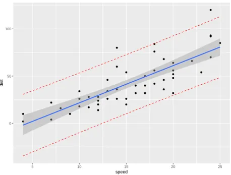
0 50 100

5 10 15 20 25

speed

dist

Figure 3.1: Regression line, confidence interval and prediction interval for a simple regression of the speed of cars (Y) and the distances taken to stop (X). In blue there is the estimated regression line in blue. Confidence interval bands (forE[Y]) are reported in the gray area. Prediction interval bands (for Y) are reported in red. Note that the red bands include the gray area.

The 100(1−α)% confidence interval for E[Y] at X=x0 is given by ˆ

y₀±tα/2;(n−p−1)

q

s²(x₀(X^TX)⁻¹x^T₀)

The 100(1−α)% prediction interval for Y atX=x0 is given by ˆ

y₀±tα/2;(n−p−1)

q

s²(1 +x₀(X^TX)⁻¹x^T₀).

(35)

3.3. Predictions

This result is due to the fact that, as y₀ is unknown, the total variance is s² +var(ˆy₀). Of course, if there is more than one new observation, we must take in account the diagonal elements ofp

s²(1 +X₀(X^TX)⁻¹X^T₀) and ps²(X₀(X^TX)⁻¹X^T₀).

Note that we consider the new individual as a row vector x0 = [1, x₀₁, . . . , x_0p]. For this reason we use the notation X₀(XX)⁻¹X^T₀). In general, we should consider the new observation as x₀ = [1, x₀₁, . . . , x_0p]^T, hence usually the notation is (X^T₀(XX)⁻¹X0).

Inference for the reduced model

Usually in a multiple regression setting there will be at least some X variables that are related to y, hence the F-test of goodness of fit usually results in rejection of H0.

A useful test is one that allows the evaluation of a subset of the explanatory variables relative to a larger set.

Suppose to use a subset of q variables, and test the null hypothesis H₀ :β₁ =β₂, . . . , β_q= 0 with q < p.

The model with all thepexplanatory variables is called thefull model, while the model that holds under H₀ with (p−q) explanatory variables is called the reduced model:

y=β0+β(q+1)+β(q+2)+. . .+βp+e.

If the null hypothesis H0 :β1 =β2, . . . , βq = 0 is true, then the statistic F = (SSR−SSRR)/q

SSE/(n−p−1) = (SSER−SSE)/q SSE/(n−p−1)

has an F distribution with q and (n − p − 1) degrees of freedom. This test is often calledpartial F test. In the above formulation, SSRR and SSER

represent the regression and the residual sum of squares of the reduced model, respectively.

The same statistic can be written in terms of R² and R²_R, where R²_R is the coefficient of multiple determination of the reduced model:

F = (R²−R²_R)/q (1−R²)/(n−p−1).

27

(36)

This procedure helps to make a choice between two nested models estimated on the same data (see, for example Chatterjee & Hadi, 2015). A set of models are said to be nested if they can be obtained from a larger model as special cases. The test for these nested hypotheses involves a comparison of the goodness of fit that is obtained when using the full model, to the goodness of fit that results using the reduced model specified by the null hypothesis. If the reduced model gives as good a fit as the full model, the null hypothesis, which defines the reduced model, is not rejected.

The rationale of the test is as follows:

in the full model there are p+ 1 regression parameters to be estimated. Let us suppose that for the reduced model there are k distinct parameters. We know thatSSR ≥SSR_Rand SSE_R≥SSE because the additional parameters (variables) in the full model cannot increase the residual sum of squares (R² is not decreasing when the number of predictor increases).

The difference SSE_R−SSE represents the increase in the residual sum of squares due to fitting the reduced model. If this difference is large, the reduced model is inadequate, and we tend to reject the null hypothesis. In our notation, we used q to denote the subset of variables of the full model we wish to test their simultaneous equality to zero.

If we denote withkthe number ofparameters estimated in the reduced model (hence, including the intercept), thenq = (p+ 1−k).

The meaning of the partial F test is the following: can y be explained adequately by fewer variables? An important goal in regression analysis is to arrive at adequate descriptions of observed phenomenon in terms of as few meaningful variables as possible. This economy in description has two advantages:

it enables us to isolate the most important variables;

it provides us with a simpler description of the process studied, thereby making it easier to understand the process.

The principle of parsimony is one of the important guiding principles in regression analysis. Probably, you will study many techniques of model selection and variable selection (stepwise regression, best subset selection, etc.) in studying other quantitative disciplines.

(37)

3.4 Illustrative example, part 4

Consider the toy example introduced in section 2.3.1. Suppose to have a new observation x₀ = [15.18, 2]. Remember that

(X^TX)⁻¹ =





31.31 −2.09 0.10

−2.09 0.14 −0.01 0.10 −0.01 0.02



,and ˆβ =





57.76 2.24

−4.52



.

Moreover, from Chapter 2.4.1 we know thatSSE = 513.80, and from Section 3.2 we know that s² = 73.40 and the covariance matrix is





2297.99 −153.76 7.52

−153.76 10.49 −0.98 7.52 −0.98 1.35



.

Hence, we can made the prediction:

ˆ

y₀ =x₀βˆ = ˆβ₀+ ˆβ₁x₀₁+ ˆβ₂x₀₂

=

1 15.18 2

×





57.76 2.24

−4.52





= 57.76 + 2.24×15.18 +−4.52×2

= 82.66

Let’s determine both the confidence interval and the prediction interval. First we set the confidence level to be, say, equal to 95% and determine the quantile of the t distribution withn−p−1 = 7 degrees of freedom that leaves 2.5%

probability on the tails. This value is equal to t_0.025,7 = 2.36. Then we compute the quantity, that we call C,

C=t0.025,7

q

s2(x0(X^TX)⁻¹x^t₀)

= 2.36× v u u ut73.40×





1.00 15.18 2.00

×





2297.99 −153.76 7.52

−153.76 10.49 −0.98 7.52 −0.98 1.35



×



 1.00 15.18 2.00









= 11.35

The confidence interval for ˆY₀ is then

29

(38)

ˆ

y₀ lower bound upper bound

82.66 82.66 - 11.35 = 71.31 82.66 + 11.35 = 94.01

To compute the prediction interval we must computeC in other way:

C=t0.025,7

q

s2(1 + (x0(X^TX)⁻¹x^t₀))

= 2.36× v u u ut73.40×



1 +





1.00 15.18 2.00

×





2297.99 −153.76 7.52

−153.76 10.49 −0.98 7.52 −0.98 1.35



×



 1.00 15.18 2.00













= 23.22

The prediction interval for Y₀ is then ˆ

y₀ lower bound upper bound

82.66 82.66 - 23.22 = 59.44 82.66 + 23.22 = 105.88

As you can see, the prediction interval, for the same point estimate, is wider than the confidence interval.

Inference for the reduced model will be seen in the next chapter.

(39)

Chapter 4

Linear regression: summary example 1

4.1 The R environment

In this chapter we try to practically see what we defined in the previous chapters. All the computations have been made in R environment (R Devel- opment Core Team, 2006). R is a language and environment for statistical computing and graphics. Students can reproduce the reported examples by copying and pasting the reported syntax. For an introduction to R, students can refer to Paradis (2010).

4.2 Financial accounting data

Financial accounting data (Jobson, 1991, p.221) contain a set of financial indicators for 40 companies in UK, as summarized in table 4.2. We assume that the Return of capital employed (RET CAP) depends on all the other variables.

Data can be accessed by downloading the file J tab42.rda from http://

wpage.unina.it/antdambr/data/MPQE/. Once the file has been downloaded in the working directory, the data set can be loaded by typing

> load("Jtab42.rda")

(40)

Variable Definition RETCAP Return of capital employed

WCFTDT Ratio of working capital flow to total debt LOGSALE Log to base 10 of total sales

LOGASST Log to base 10 of total assets CURRAT Current ratio

QUICKRAT Quick ratio

NFATAST Ratio of net fixed assets to total assets FATTOT Gross fixed assets to total assets PAYOUT Payout ratio

WCFTCL Ratio of working capital flow to total current liabilities GEARRAT Gearing ratio (debt-equity ratio)

CAPINT Capital intensity (ratio of total sales to total assets) INVTAST Ratio of total inventories to total assets

Table 4.1: Financial accounting data

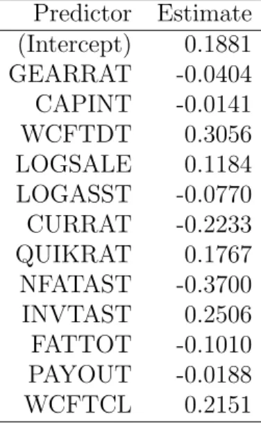
Let’s give a look to the results first. The estimated regression coefficients are Predictor Estimate

(Intercept) 0.1881 GEARRAT -0.0404 CAPINT -0.0141

WCFTDT 0.3056

LOGSALE 0.1184 LOGASST -0.0770 CURRAT -0.2233 QUIKRAT 0.1767 NFATAST -0.3700 INVTAST 0.2506 FATTOT -0.1010 PAYOUT -0.0188

WCFTCL 0.2151

Each β_j should be interpreted as the expected change in y when a unitary change is observed in xj while all other predictors are kept constant.

The intercept is the expected mean value ofy when all x_j = 0.

In this case each coefficient of an explanatory variable measures the impact of that variable on the dependent variable RETCAP, holding the other variables fixed. For example, the impact of an increase in WCFTDT of one unit is a change in RETCAP of 0.3056 units, assuming that the other

(41)