Mathematical Structures in Computer Science

Science

http://journals.cambridge.org/MSC

Additional services for

Mathematical Structures in Computer Science:

Email alerts: Click here Subscriptions: Click here Commercial reprints: Click here Terms of use : Click here

On the reication of semantic linearity

MARCO GABOARDI, LUCA PAOLINI and MAURO PICCOLO

Mathematical Structures in Computer Science / FirstView Article / November 2014, pp 1 - 39 DOI: 10.1017/S0960129514000401, Published online: 10 November 2014

Link to this article: http://journals.cambridge.org/abstract_S0960129514000401

How to cite this article:

MARCO GABOARDI, LUCA PAOLINI and MAURO PICCOLO On the reication of semantic linearity. Mathematical Structures in Computer Science, Available on CJO 2014 doi:10.1017/

S0960129514000401

Request Permissions : Click here

doi:10.1017/S0960129514000401

On the reification of semantic linearity

M A R C O G A B O A R D I^†, L U C A P A O L I N I^‡ and M A U R O P I C C O L O^‡

†School of Computing, University of Dundee, Dundee, DD1 4HN, Scotland, U.K.

‡Dipartimento di Informatica, Universit`a degli Studi di Torino, C.so Svizzera 185, 10149 Torino, Italy Email:paolini@di.unito.it

Received 21 April 2013; revised 19 November 2013

Linearity is a multi-faceted and ubiquitous notion in the analysis and development of programming language concepts. We study linearity in a denotational perspective by picking out programs that correspond to linear functions between domains.

We propose a PCF-like language imposing linear constraints on the use of variable to program only linear functions. To entail a full abstraction result, we introduce some higher-order operators related to exception handling and parallel evaluation. We study several notions of operational equivalence and show them to coincide with our language.

Finally, we present a new operational evaluation of the language that provides the base for a real implementation. It exploits the denotational linearity to provide an efficient evaluation semantics SECD-like, that avoids the use of closures.

1. Introduction

Linearity is a key tool to support a conscious use of resources in programming languages.

A non-exhaustive list of its uses includes garbage collection, memory management and aliasing control, description of digital circuits, process channels and messages management, languages for quantum computations, etc. A survey of several variants of linear type systems proposed in the literature is in Walker (2005). This broad spectrum of applications highlights the fact that linearity is a multi-faceted abstract concept which can be considered in different perspectives. For instance, notions of syntactical linearity can be considered when variables are used once (in suitable senses), e.g. Alves et al. (2007) and Hindley (1989). On the other hand, if redexes cannot be discarded or duplicated during reduction, like in Hindley (1989), then a kind of operational linearity is achieved. This is related to the notion ofsimple term inλ-calculus (Klop 2007), which suggests a kind of linearity on reductions, unrelated from a specific strategy.

Although ideas that can be tracked to linearity have been implicitly used in pro- gramming languages for many years, the introduction of linear logic (Girard 1987) is a redoubtable milestone in this setting. Linear logic arises from a sharp semantic analysis of stable domains where stable functions have been decomposed into linear functions and exponential domain constructors. Such a decomposition is patently reflected in the syntax of linear logic. Moreover, it suggests a new approach to linearity: denotational linearity. In a programming perspective, denotational linearity says that programs (i.e.

closed terms) should correspond via a suitable interpretation to linear function on some specific domains, e.g. the linear models introduced in Bucciarelliet al. (2010), Bucciarelli and Ehrhard (1993), Girard (1987) and Huth (1993). By tackling this correspondence

minutely, some important contributions to the theory of programming can be obtained.

For instance, if the intended domain includes all the computable functions, this analysis provides Turing-complete languages with weak syntactic linear constraints on variables, and new linear operators that, in a higher-type computability perspective (Longley 2000;

Normann 2006), increase the expressivity of linear languages.

Following the denotational linearity approach, we study (recursive) linear functions in thetype theory L of coherence spaces and linear functions introduced by Girard (1987).

An attractive aspect of this type theory is the simplicity of its formulation. We present a language, named SPCF that is fully abstract for this type theory. SPCF can be described as the combination of the following ingredients.

— A core PCF-like language, named core-SPCF, characterized by a constrained man- agement of variables and by an operational semantics based on a careful evaluation of program mixing call-by-name and call-by-value. This core language is Turing complete and can be soundly interpreted inL.

— A higher-order operator, named which?, that corresponds to a primitive form of exception handling.which? permits to obtain besides the result of an evaluation also some information about the way the result is computed.

— A higher-order operator, namedet-or, that permits to explore in parallel different program branches. A distinguished feature ofet-oris that it permits to share some information between the different branches.

The combination of the core language with the two higher-order linear operators which? and et-or is essential to gain a finite definability result (Curien 2007), i.e. the definability of all the finite cliques of the considered linear model. The finite definability result is not only the key ingredient to obtain the full abstraction result, but it is also important to show the programming patterns that the language offers. The importance of the full abstraction comes from the fact that it allows us to reason about program in a compositional way. Moreover, full abstraction allows us also to prove the coincidence of three different definitions of operational equivalence. These definitions make the reasoning simpler on the equivalence between programs by permitting to consider restricted families of contexts.

An interesting remark is that SPCF is neither syntactically linear nor operationally linear in tight sense, albeit its finitary fragment (the set of programs which does not involve recursion) respects some syntactical and operational forms of linearity (see Remark 1).

We present SPCF by means of a self-explanatory operational semantics that, quite inefficiently, requires for some operators an infinite branching search in the evaluation tree. Then, we show that SPCF programs can be evaluated in an efficient way by means of another abstract machine that traces out and records linear information to finitely prune the infinite branching search tree of the evaluation ofSPCF. The latter tracing operational machine is a very concrete by-product of our results, since it tailors on denotationally linear constraints a very efficient evaluation of a Turing-complete

programming language endowed of parallel features and exception-like mechanism, namelySPCF.

The study of the relations between languages and models is a classic theme in denotational semantics (Curien 2007; Ong 1995). The full abstraction for PCF has led to the development of very sophisticated semantics techniques (as Abramsky et al.

(2000) and Hyland and Ong (2000)) and revealed relevant programming principles and operational constructions. In particular, several works have studied how to extend PCF by different operators in order to achieve full abstraction compared to some classical models.

For example, this approach has been followed by Plotkin (1977) for the continuous Scott model, by Berry and Curien (1982) for the sequential algorithms model, by Abramsky and McCusker, (1996) for a particular game model, by Longley (2002) for the strongly stable model and by Paolini (2006) for the stable model. Remark that all higher-type operators introduced in the works above cannot be directly interpreted in the linear model. This is another motivation for our search for new operators.

Many linear languages with different goals have been proposed so far in the literature.

Recently, in the studies of syntactical linearity, Alves et al., (2006; 2007; 2010) have proposed several syntactical linear languages in order to characterize different classes of computable functions. To explore their extension, higher-type semantically-motivated operators, is another interesting open problem.

Two PCF-like languages embedding linearity notions have been proposed in Bierman (2000) and Bierman et al. (2000). These languages are not denotationally linear, in the sense that not all their closed terms are in correspondence with linear functions of a suitable domain. In particular, they cannot be interpreted in the linear model considered here. Despite this fact, the authors of Bierman (2000) and Biermanet al.(2000) give some interesting results on the relations between several forms of operational reasoning, in the context of the linear decomposition. Our results on the coincidence of three operational equivalences can be viewed as further contributions in those topics.

The results we present in this paper extend and complete our previous works: Gaboardi and Paolini (2007), Gaboardi et al. (2011) and Paolini and Piccolo (2008). The core- SPCF language and thewhich? operator were first introduced by Gaboardi and Paolini (2007) and Paolini and Piccolo (2008), respectively. Paolini and Piccolo (2008) proved the language combining these two components, named SPCF, correct for the type theory L. Moreover, they showed a full abstraction result for stable closed terms, i.e. terms not containing free occurrences of a particular kind of variables used for recursion. Gaboardi et al. (2011) extended SPCF by means of the et-or operator obtaining in this way the full abstraction for terms that can contain free occurrences of stable variables. The enhanced tracing operational machine we present in this paper greatly improves the efficiency of tracing operational machine defined in Gaboardi et al.(2011).

1.1. Synopsis

In Section 2, we introduce the core-SPCF language, the linear type theory L and the interpretation. We show that the interpretation is sound and that a full abstraction result holds for stable closed terms. In Section 3, we show that for the core language of

Section 2, a more general full abstraction result does not hold. In Section 4, we introduce the two operators which? and et-or, completing in this way the introduction of SPCF. We provide some programming examples and we prove finite definability and full abstraction for it. In Section 5, we show the coincidence of three operational equivalences.

In Section 6, we give an abstract machine forSPCF that traces the linear use of terms.

This provides the base for an efficient implementation of our language.

2. The core of a linear programming language

As described in the introduction, following the denotational linearity approach, our aim is to design a programming language corresponding to a particular linear type theoryL.

Here we start by presenting a core part of this language, named core-SPCF, then we present the type theoryLand we show how core-SPCF can be soundly interpreted inL and how a limited form of full abstraction can be obtained.

The types of the language are defined as following:

σ, τ ::= ι (natural numbers)

| σ(τ (arrow or function type).

As usual,(associates to the right soσ1(σ2(σ3 is read asσ1((σ2(σ3).

Let Var^σ be a numerable set of variables of type σ. If σ = ι then, let SVar^σ be a numerable set of variables disjoint from Var^σ. Variables in Var^ι are named ground variables. Variables in Var =

σ,τ∈TVar^σ(τ are named linear variables. Variables in SVar =

σ=ιSVar^σ are namedstable variables. Latin lettersx^σ,y^σ,f^σ, . . .denote variables in Var^σ. Moreover,z^σ₀,z^σ₁,z^σ₂, . . .denote stable variables. Last,{ is a wild-card for all the variables.

Definitiona 1. Core-SPCFpre-termsare defined by the following grammar:

M ::= {^τ variable

| 0 zero

| s successor

| p predecessor

| if M M M conditional

| MM application

| λx^σ.M λ-abstraction

| μz^σ.M μ-abstraction

We write n for s(· · ·(s0)· · ·) where s is applied n-times to 0, and we denote N = {0, . . . ,n, . . .} the set of numerals. When the type information is irrelevant, we will omit type labels. We partitioned variables in three main categories: Var^ι, Var,SVar. Other choices are possible, but we preferred this one in order to emphasize their differences.

The two kinds of abstraction act as binders in the standard way, λ-abstraction binds ground and linear variables (however, the first set of variables entails a call-by-value policy and the latter a call-by-name one), while μ-abstraction binds stable ones. Free variables of any kind (FV), free linear variables (FV), free stable variables (SFV), closed

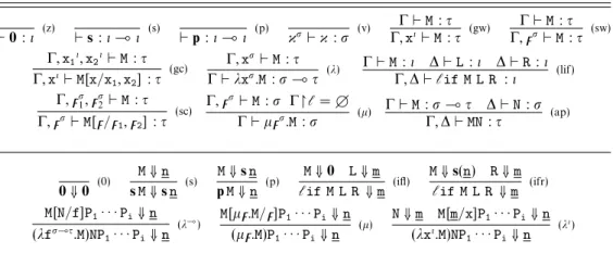
Table 1.(a) Type system and (b) operational semantics.

0:ι ^(z) s:ι(ι ^(s) p:ι(ι ^(p) {^σ{:σ ^(v)

ΓM:τ Γ,x^ιM:τ ^(gw)

ΓM:τ Γ,z^σM:τ ^(sw) Γ,x₁^ι,x₂^ιM:τ

Γ,x^ιM[x/x1,x2] :τ ^(gc)

Γ,x^σM:τ Γλx^σ.M:σ(τ ^(λ)

ΓM:ι ΔL:ι ΔR:ι Γ,Δif M L R :ι ^(lif) Γ,z^σ1,z^σ2 M:τ

Γ,z^σM[z/z1,z2] :τ ^(sc)

Γ,z^σM:σ Γ=6 Γμz^σ.M:σ ^(μ)

ΓM:σ(τ ΔN:σ Γ,ΔMN:τ ^(ap)

0⇓0 ⁽⁰⁾

M⇓n sM⇓sn ^(s)

M⇓sn pM⇓n ^(p)

M⇓0 L⇓m if M L R ⇓m ^(ifl)

M⇓s(n) R⇓m if M L R ⇓m ^(ifr) M[N/f]P1· · ·P_i⇓n

(λf^σ(τ.M)NP1· · ·P_i⇓n ^(λ

() M[μz.M/z]P1· · ·P_i⇓n (μz.M)P1· · ·P_i⇓n ^(μ)

N⇓m M[m/x]P1· · ·P_i⇓n (λx^ι.M)NP1· · ·P_i⇓n ^(λ

ι)

and open terms are defined as expected. M[N/{] denotes the capture-free substitution of all free occurrences of{inMbyN. As usual application associates to the left, i.e.MN1. . .Nk

abbreviates (. . .((MN₁)N₂). . .Nk) and we routinely omit parenthesis as we safely can.

Core-SPCFterms are pre-terms that are well typed. We consider typing judgments of the shape Γ M:σ where M is a pre-term,σ is a linear type and Γ is abasis, that is a finite list of variables in Var∪SVar, where each variable appears at most once. We denote ΓS(resp Γι, Γ) the restriction of the basis Γ containing only variables inSVar (resp.

in Var^ι, Var). We denote Γ,Δ, Γ∪Δ and Γ∩Δ the disjoint union, the union and the intersection of two basis respectively. We writeM^σ to signify that there is a basis Γ such that ΓM:σ.

Definitiona 2. The pre-terms typable by using the type system in Table 1(a) are theterms of core-SPCF.

We remark that the type system contains weakening and contraction rules only for ground and stable variables (viz. (gw), (sw), (gc) and (sc)), while linear variables are managed by means of linear-typing rules (the ruleifis additive). Therefore, it is easy to check that the following rules are derivable rules in our system.

Γ1M:σ(τ Γ2N:σ Γ1∩Γ2=6. Γ1∪Γ2 M N:σ

Γ₀M:ι Γ₁P:ι Γ₂ Q:ι Γ₁= Γ₂ Γ₀∩Γ₁=6. Γ0∪Γ1∪Γ2if M P Q :ι

A closed term of ground type is called program andPdenotes the set of all programs.

Definitiona 3. Theevaluation relation ⇓between programs of core-SPCF and numerals is the smallest relation inductively satisfying the rules of Table 1(b). For any program M, if there exists a numeralnsuch thatM⇓nthen we say thatMconverges and we writeM⇓. Otherwise, we say that itdiverges and we writeM⇑.

We remark that the evaluation is carried out in a call-by-name fashion by the rule λ⁽, and in a call-by-value fashion by the rule λ^ι. Patently all terms appearing in the evaluation rules are well typed. To be more precise, in the ruleλ⁽, we are assuming that τ=σ₁(. . .(σ_i(ιwhereσ_k is the type ofPk. Moreover, note that the evaluation of the programp0diverges.

Remark 1. Note that the finitary fragment of SPCF (i.e. the language obtained by avoiding stable variables and μ-abstractions) contains terms like λf^ι(ι.if 5(f 0) (f 1) andλf^ι(ι(ιx^ι.fxxwhich are not syntactically linear. Moreover,SPCF is not operationally linear because in the following term

(λf^ι(ι.if 5(f 0) (f 1))((λx^ι.λy^ι.y)5) the redex (λx^ι.λy^ι.y)5is duplicated during the evaluation.

We name some terms. LetΩ^ι :::===p0 and inductively, if σ₀=μ₁( . . .(μ_m (ι for somem∈N, then

Ω^{σ0(...(σn(ι}:::===λx^σ₀⁰. . .x^σ_nⁿ.if(Ω^{σ1(...(σn(ι}x^σ₁¹. . .x^σ_nⁿ)(x₀Ω^μ1. . .Ω^μm)(x₀Ω^μ1. . .Ω^μm).

If σ = ι then it is possible to define Ω^σ as μz^σ.z and, still, to satisfy the Lemma 1.

Nevertheless, the crucial use ofΩ^σ is to define the approximants, i.e. terms approximating μ-abstraction that avoids the use of (additional)μ-abstractions. In this way, we can prove the Lemma 5 by adapting the Tait technique used in Plotkin (1977). By using Ω^σ, it is possible to define approximants of a term having shapeμz.M^σ as follows,

μ⁰z.M^σ:::===Ω^σ, μⁿ⁺¹z.M^σ:::===M[μⁿz.M/z].

It is easy to check that theμ-abstractions inμⁿz.M^σ are strictly less than that inμz.M^σ. Lemma 1. Let M^σ₀⁰, . . . ,M^σ_m^m be a sequence of closed terms (m>0).

1.Ω^{σ0(...(σm(ι}M0. . . Mmis a program andΩ^{σ0(...(σm(ι}M0. . .Mm⇑. 2. Let (μz.P^σ)M0. . .Mmbe a program.

(μz.P^σ)M₀. . .Mm⇓n if and only if (μ^k+1z.P^σ)M₀. . .Mm⇓n, for somek∈N.

Proof. (1) The proof can be done by induction on m. (2) Both implications can be proved by induction on derivations proving the hypothesis.

2.1. Pairing

In the following sections, we need pairing and projections operators on natural numbers.

This can be defined as follows. If m, n∈Nthen< m, n >= 2^m(2n+ 1)−1 is our pairing function. Projections fromz∈Ncan be defined by functions

pi1(z) = min

x6z[(∃y)₆z(z=< x, y >)] ; pi2(z) = min

y6z[(∃x)₆z(z=< x, y >)].

Such functions induce a bijection, details can be found either, in p.41, p.73 of Cutland (1980) or in p.47 of Davis and Weyuker (1983). The reader can easily verify that

Sum=μz.λx^ιy^ι.if x y(z(px) (sy)) Prod≡μz.λx^ιy^ι.if x 0(Sum y(z(px)y)) Exp2≡μz.λx^ι.if x 1(Prod 2(z(px)))

respectively define the addition, the multiplication and the exponentiation of base 2.

Hence, the above function< , >is defined by the program

−,− ≡λx^ιy^ι.p

Prod(((Exp2 x)))(((s(Prod 2 y)))) .

Clearly, our pairing-program is total and correct i.e.n,m ⇓<n,m>for all numeralsn,m.

So, we will writeM⇓ n,m, for someM, has a shorthand for∃k, M⇓kandn,m ⇓k.

The definition of the termsπππ₁ andπππ₂ corresponding to projection (i.e. which are such thatπππ1 n,m ⇓nandπππ2 n,m ⇓m) turns out to be an easy exercise and it is left to the reader. Again, we writeM⇓πππ_in(i∈[1,2]) to mean∃k,M⇓kandπππ_in⇓k.

2.2. Operational equivalence

There is a notion of program equivalence which programmers understand well: two program fragments are equivalent if they can always beinterchangedwithout affecting the visible or observable outcome of the computation.

The set ofσ-context Ctxσ is defined as:

C[^σ] ::= [^σ]|{^τ |0|s|p|if C[^σ]C[^σ]C[^σ]|(C[^σ]C[^σ])|(λx^σ.C[^σ])|μz.C[^σ].

C[N^σ] denotes the result obtained by replacing all the occurrences of [^σ] in the contextC[^σ] by the termN^σ and by allowing the capture of its free variables.

Definitiona 4 (standard operational equivalence). LetM^σ,N^σ be terms.

1.M/σNwhenever, for all C[^σ] s.t.C[M],C[N]∈P, ifC[M]⇓nthenC[N]⇓n.

2.M≈σNif and only ifM/σNandN/σM.

The above definition is standard, however, we introduce an alternative equivalence definition that will allow to study the formal relationship between the two binders we introduced.

Definitiona 5 (fix-point operational equivalence). LetM^σ,N^σ be such that SFV(M),SFV(N)⊆ {z^σ₁¹, . . . ,z^σ_nⁿ}.

1.M.σNwhenever, for all P^σ₁¹, . . .P^σ_nⁿ, for allC[^σ] s.t.

C[M[P₁/z1, . . . ,Pn/zn]],C[N[P₁/z1, . . . ,Pn/zn]] ∈ P if C[M[P₁/z1, . . . ,Pn/zn]] ⇓ n then C[N[P1/z1, . . . ,Pn/zn]]⇓n.

2.M∼σNif and only ifM.σNandN.σM.

It is easy to verify that .σ is a preorder and ∼σ is an equivalence. Note that the comparison between the fix-point operational equivalence and the standard one is not immediate, since there is no obvious way to implement substitution of a stable variable with an arbitrary term. This issue will be discussed in detail in Section 6.

2.3. Coherence spaces

We are interested in the least full subcategory L of coherence spaces, including the flat domain of natural numbers and the coherence spaces of linear functions between domains in the category itself. Coherence spaces are a simple framework for Berry’s stable functions (Berry 1978), developed by Girard (1987). This section does not aim to provide an exhaustive presentation of these arguments, it just aims to make the paper self-contained. More details can be found in Girard (1986, 1987) and Girardet al.(1989).

Acoherence space X is a pair |X|, X, where |X| is a set of tokens called the web of X and X is a reflexive and symmetric relation between tokens of |X| called the coherence relationon X. Thestrict incoherence_X is the complementary relation ofX; theincoherence _X is the union of relations_X and =; the strict coherence _X is the complementary relation of _X. A clique x of X is a subset of |X| containing pairwise coherent tokens. The set of cliques ofX is denotedCl(X), while the set of finite cliques is denotedClfin(X). Two cliquesx, y∈Cl(X) arecompatible whenx∪y∈Cl(X).

IfX is a coherence space thenCl(X) form a cpo (indeed, a Scott-domain) with respect to the set-theoretical inclusion. In particular,

— 6∈Cl(X) is the bottom element and{a} ∈Cl(X), for each a∈ |X|,

— ify⊆xandx∈Cl(X) theny ∈Cl(X),

— ifD⊆Cl(X) is directed then

D∈Cl(X),

— the set of compact elements isCl_fin(X).

Definitiona 6. LetX andY be coherence spaces.

1. Thelinear implicationX (Y is the coherence space having|X(Y|=|X| × |Y|as web, while (a, b)ΠX(Y (a, b) iffaΞX a impliesbΠY b.

2. Alinear morphismbetweenX andY is an element ofCl(X (Y).

3. Thetensor productX⊗Y is the coherence space having |X⊗Y|=|X| × |Y|as web, while (a, b)Ξ_X⊗Y (a, b) ifaΞXaandbΞY b.

We denote with LinCoh the category whose objects are coherence spaces and whose morphisms are linear morphisms between coherence spaces. (LinCoh,⊗,1,() is a sym- metric monoidal closed category, where1is the coherence space having a singleton set as web.

Definitiona 7. Let X, Y be two coherence spaces. A function f : Cl(X) → Cl(Y) is continuouswhenever, it is monotone and it commutes with the union of directed sets of cliques. A continuous functionf :Cl(X)→Cl(Y) isstablewhen∀x, x∈Cl(X), xand x compatible impliesf(x∩x) =f(x)∩f(x). A functionf :Cl(X)→Cl(Y) islinearwhen it is stable (so, continuous),f(6) =6and for allx, x∈Cl(X), ifx andx are compatible thenf(x∪x) =f(x)∪f(x).

Linear morphisms are in bijection with linear functions between cliques.

Thetrace of a linear functionf:Cl(X)→Cl(Y) isTr(f) ={(a, b)|a∈ |X|, b∈f({a})}.

Givent∈Cl(X (Y) andx∈Cl(X), let us define the map F(t) :Cl(X)→Cl(Y) as F(t)(x) ={b∈ |Y| | ∃a∈x,(a, b)∈t}. (1)

Proposition 1.

1. Iff :Cl(X)→Cl(Y) is a linear function thenTr(f)∈Cl(X(Y).

2. Ift∈Cl(X (Y) thenF(t) :Cl(X)→Cl(Y) is a linear function.

3.Tr(F(t)) =t, for allt:Cl(X(Y).

4.F(Tr(f)) =f, for allf :Cl(X)→Cl(Y).

The basis of our model is the countable flat domain. LetNdenotes the space of natural numbers, namely (|N|, N) such that |N|:::===N(the latter is the set of natural numbers) andm Nnif and only ifm=n, for allm, n∈ |N|.

Definitiona 8 (linear model). The linear model L is the type structure generated by the coherence spaceNand the arrow(.

To provide the interpretation of the recursion in core-SPCF, we discuss the fix-point operator on coherence domain. More precisely, ifX is a coherence space then we look for fixX : (Cl(X)→Cl(X))→Cl(X) such thatfixX(f) =f(fixX(f)) for all stable functions f :Cl(X) →Cl(X). Given any coherence spaces X, Y, we remind that the set of stable functions between Cl(X) and Cl(Y) together with stable ordering^† form a Scott domain.

Thus we define a family of maps^‡ fixⁿ_X : (Cl(X) → Cl(X)) → Cl(X) by induction on n∈N:

fix⁰_X =–f:Cl(X)→Cl(X).6 fixⁿ⁺¹_X =–f :Cl(X)→Cl(X).f(fixⁿ_X(f)).

By using Knaster–Tarski fix point theorem, we can definefixX=

nfixⁿ_X. In the sequel, we will omit the subscriptX onfixX when it is clear from the context or uninteresting.

Proposition 2. Let X be a coherence space and letf :Cl(X)→Cl(X),g:Cl(X)→Cl(N) be two stable functions and let p∈N. Ifg(fix(f)) ={p}, then there is k ∈Nsuch that g(fix^k(f)) ={p}.

We stress the fact that fix is a stable function which is not linear. We use fix in a restricted way, it is applied only to stable endo-functions inL, and it gives back traces of linear functions. The Kleisli category on the finite-clique comonadLinCoh! is equivalent to the category of coherence spaces and stable functions. This category is Cartesian closed and it admits a least fix point operator, which corresponds to the above defined fix.

2.4. Linear interpretation

We define a standard interpretation (Plotkin 1977) such that ι =N and σ ( τ= σ ( τ. An environment ρ ∈ Env is a total function mapping a variable x^σ in a token a∈ |σ| and a stable variable z^σ in a finite cliquex∈Clfin(σ). We remark that

†Letf, g:Cl(X)→Cl(Y) two stable functions. Thestable orderingfgis defined as∀x, y∈Cl(X),x⊆y impliesf(x) =f(y)∩g(x).

‡LetAandBbe two sets, letxbe an element ofAand letE(x) be an expression that may containxand corresponding to an element ofB.–x:A.E(x) is the function fromAtoBmapping any elementx∈Ainto the elementE(x)∈B, that is the functionf:A→Bsuch thatf(x) =E(x). In p. 49 of Gunter (1992), the notationx→E(x) is used with the same meaning of–x.E(x).

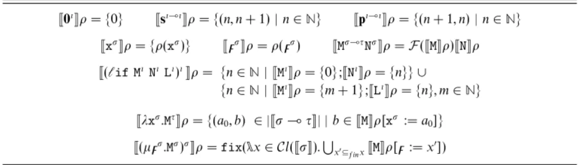
Table 2.Linear interpretation map.

0^ιρ={0} s^ι(ιρ={(n, n+ 1)|n∈N} p^ι(ιρ={(n+ 1, n)|n∈N}

x^σρ={ρ(x^σ)} z^σρ=ρ(z^σ) M^σ(τN^σρ=F(Mρ)Nρ (if M^ιN^ι L^ι)^ιρ= {n∈N|M^ιρ={0};N^ιρ={n}} ∪

{n∈N|M^ιρ={m+ 1};L^ιρ={n}, m∈N}

λx^σ.M^τρ={(a0, b) ∈ |σ(τ| |b∈Mρ[x^σ:=a0]}

(μz^σ.M^σ)^σρ=fix(–x∈Cl(σ).

x⊆finxMρ[z:=x])

the interpretation of x^ι cannot be associated to an empty cliques, so it is subjected to restrictions (see cases 4 and 5 of Lemma 2). The set of environments is denoted by Env.

Leta be a sequence of tokens of a coherence space, letx be a sequence of non-stable variables of the same length ofa;ρ[x:=a] is the environment such thatρ[x:=a](x) =ai

in case x is the ith element ofx, otherwise ρ[x:=a](x) = ρ(x). Ifx is a sequence of finite cliques andzis a sequence of stable variables of the same length then ρ[z:=x] is defined likewise. We will writex⊆finy whenx⊆y withxfinite.

Definitiona 9. Let M^σ,N^σ and ρ ∈Env. The linear interpretation M^σ: Env→Cl(σ) is defined in Table 2 usingF as defined inEquation 1and fixwhich is the least fix point operator.

Looking at the interpretation, we justify the introduction of stable variables. Those variables are used in order to program continuous (w.r.t. stable order) non-strict functions from a linear coherence space L to itself, so their fix-points will be always an element of L. Notice that, syntactically, a stable variable will be used without linear constraints.

We do not permit to λ-abstract stable variables, we use them only in order to obtain fix-points. Permitting the λ-abstraction of stable variable would produce terms defining non-linear functions, which is against our wishes.

Two terms M^σ and N^σ are denotationally equivalent if and only if M^σρ = N^σρ for every ρ. The interpretation of closed terms is invariant with respect to environments, thus in such cases the environment can be omitted. Next lemmas are standard. The basic properties of aλ-model are recalled in Lemma 2.

Lemma 2. Let M^σ,N^τandρ, ρ∈Env.

1. Ifρ(z)⊆ρ(z) for eachz∈SFV(M), thenMρ⊆Mρ. 2. IfM^σ[N/z^τ]∈SPCF thenM^σ[N/z^τ]ρ=

x⊆fin^NρMρ[z^τ:=x].

3. IfM^σ[N/x^τ]∈SPCF withτ=ιthenM^σ[N/x^τ]ρ=

a∈^NρMρ[x:=a].

4. IfM^σ[n/x^ι]∈SPCF thenM^σ[n/x^τ]ρ=Mρ[x:=n].

5.(λx^ι.M)n=M[n/x^ι]. 6.(λf^σ.M)N=M[N/f^σ].

7.if 0 L R=Landif n+1 L R=R.

8.μz^σ.M=M[μz^σ.M/z^σ].

9. Ifσ=τ,C[^σ]∈Ctxσ,C[M],C[N]∈PandMρ=NρthenC[M]=C[N].

Proof. (1)–(4) follow by induction on the structure of M^σ. The proofs of (5)–(8) follow by definition of interpretation and by points (2), (3) and (4). The proof of (9) follows by induction on the structure ofC[^σ].

As usual, an approximation theorem for finite fixpoint semantics holds.

Lemma 3.

1.μ^kz.Mρ=fix^k(–x∈Cl(σ).

x⊆finxMρ[z:=x]).

2.μz.M^σρ=

n∈Nμⁿz.M^σρ, for allσ∈T.

Proof. (1) Obvious. (2) Sinceμⁿ⁺¹z.M^σρ=M^σρ[z:=μⁿz.M^σρ], the proof is easy.

Theorem 1. IfM⇓nthenM=n.

Proof. By induction on the derivation of M⇓ n. Lemma 2 is crucial to deal with the various inductive steps.

2.5. Adequacy and correctness

The denotational semantics is said to beadequatewhenM=nandM⇓nare logically equivalent for any programMand numeraln. We straightforward adapt a proof of Plotkin (1977) for Scott-domains, based on a computability argument in Tait style.

Definitiona 10. The ‘computability predicate’ is defined by the following cases.

— Case FV(M^σ) =6.

– Subcaseσ=ι. Comp(M^ι) if and only if∀n, M=nimpliesM⇓n.

– Subcaseσ =μ(τ. Comp(M^μ(τ) if and only if Comp(M^μ(τN^μ) for each closedN^μ such that Comp(N^μ).

— Case FV(M^σ) ={{^τ₁¹, . . . ,{^τnⁿ}, for somen>1.

Comp(M^σ) if and only if Comp(M[N1/{1, . . . ,Nn/{n]) for each closedN^τ_iⁱ s.t. Comp(N^τ_iⁱ).

Lemma 4 states a standard equivalent formulation of computability predicate.

Lemma 4. Let M^{τ1(···(τm(ι} and FV(M) ={{^μ1¹, . . . ,{^μnⁿ}^{(n, m}∈N). Comp(M) if and only if M[N1/{1, . . . ,Nn/{n]P₁. . .Pm=n implies M[N₁/{1, . . . ,Nn/{n]P₁. . .Pm⇓nfor each closed N^μ_iⁱ andP^τ_j^j such that Comp(Ni) and Comp(Pj) wherei6n, j6m.

We remark that we consider substitution to all kinds of free variables.

Lemma 5. IfM^σ is a term of core-SPCF then Comp(M^σ).

Proof. By induction on the shape ofM. We detail the most interesting cases.

— M={. Letσ =τ1 (· · ·(τm (ι, where m∈N. Let P^σ and N^τ_iⁱ for 16i 6m be closed terms such that Comp(P^σ) and Comp(N^τ_iⁱ). By definition, Comp(P^σ) implies that, ifPN1· · ·Nm=nthenPN1· · ·Nm⇓n, by definition of the computability predicate.

— M=NP. AssumeN^τ(σ andP^τ for typesσ andτ. By induction hypothesis Comp(N^τ(σ) and Comp(P^τ) and the proof follows by definition of the computability predicate.

— M=λx.Q. Assume x^μ and Q^τ for types μ and τ. Let FV(M) = {{^μ₁¹, . . . ,{^μ_k^k} fork >0 and τ= τ₁ ( · · · (τ_h (ι, where h >0. Let N^μ₁¹, . . . ,N^μ_k^k,P^μ₀,P^τ₁¹, . . . ,P^τ_h^h be closed terms such that Comp(N_i) and Comp(P_j) for 16i 6k and 06j 6 h respectively.

Thus Comp(Q^τ[P0/x][N1/{1, . . . ,Nk/{k]P1. . .Ph), since Comp(Q^τ) holds by induction hypothesis.

Consider the case μ = ι and (λx^μ.Q^τ)[N1/{1, . . . ,Nk/{k]P0. . .Ph = n.

Clearly,Q^τ[P₀/x][N₁/{1, . . . ,Nk/{k]P₁. . .Ph=nby Lemma 2 point (6). Thus Q^τ[P0/x][N1/{1, . . . ,Nk/{k]P1. . .Ph⇓nby induction hypothesis. Therefore,

(λx^μ.Q^τ)[N1/{1, . . . ,Nk/{k]P0. . .Ph⇓n by the evaluation rule (λ⁽).

Now, suppose μ=ι and (λx^μ.Q^τ)[N₁/{1, . . . ,Nk/{k]P₀. . .Ph=n. Since linear func- tions are strict, we must haveP0=mfor some m. But Comp(P^μ₀) by induction and P0 =m imply P0 ⇓ m. HenceQ^τ[m/x][N₁/{1, . . . ,Nk/{k]P₁. . .Ph =n by Lemma 2 point (5). Q^τ[m/x][N1/{1, . . . ,Nk/{k]P1. . .Ph ⇓ n by induction hypothesis. The proof follows by applying the evaluation rule (λ^ι).

— M =if M1M2M3. Assume FV(M) = {{^σ₁¹, . . . ,{^σ_nⁿ} and let P^σ₁¹, . . .P^σ_nⁿ be closed terms such that Comp(P_i) for all i. Suppose that M[P1/{1, . . . ,Pn/{n] = m. Then, by interpretation, one of the following cases holds:

– M1[P₁/{1, . . . ,Pn/{n]=0andM2[P₁/{1, . . . ,Pn/{n]=m, – M1[P₁/{1, . . . ,Pn/{n]=k+1andM3[P₁/{1, . . . ,Pn/{n]=m.

In the first case, we have M1[P₁/{1, . . . ,Pn/{n] ⇓ 0 and M2[P₁/{1, . . . ,Pn/{n] ⇓ m by inductive hypothesis; thus we conclude by the evaluation rule (ifl). For the other case, we conclude again by using inductive hypothesis and the evaluation rule (ifr).

— M=μz.N, so the typing constraints implyM^σ,N^σ for the same typeσ =ι. Let FV(M) = {{^μ₁¹, . . . ,{^μ_k^k} for k >0 and σ =τ₁ ( · · · (τ_h (ι, where h > 0. Assume h > 1 and, N^μ₁¹, . . . ,N^μ_k^k, P^τ₁¹, . . . ,P^τ_h^h be closed terms such that Comp(N_i) and Comp(P_j) for 16i6k and 16j6h respectively. Let(μz.N^σ[N1/{1, . . . ,Nk/{k])P1. . .Ph=n. By Proposition 2, there isk such that

F fix^k

–x∈Cl(σ).

x⊆finx

M[N/{]ρ[z:=x]

(P1ρ). . .(Phρ) =n.

Hence (μz.N^σ[N₁/{1, . . . ,Nk/{k])P₁. . .Ph = (μ^kz.N^σ[N₁/{1, . . . ,Nk/{k])P₁. . .Ph for some k ∈N, by Lemma 3. Thus, μ^kz.N^σ[Q/v₁, . . . ,Q/v_m]P₁. . .Ph ⇓n, by the previous points of this lemma. The proof follows by Lemma 1.

Corollary 1 (adequacy). For all M∈P, for alln, Mρ=nρif and only ifM⇓n.

As usual the adequacy implies the correctness, i.e. the denotational equivalence implies the operational one. Note that correctness implies that our terms are strict in all arguments, for all orders.

Theorem 2 (correctness). Let M^σ,N^σ be terms of core-SPCF. If M_ρ = N_ρ, for each ρ∈Env, thenM≈^σN.

Proof. Let C[^σ] such thatC[M],C[N]∈P. If C[M]⇓nfor some valuen, thenC[M]=n by Theorem 1. Since C[N] = C[M] = n by Lemma 2, C[N] ⇓ n by adequacy. By definition of standard operational equivalence, the proof is done.

We can reuse the same argument to prove the correctness for the fix-point operational equivalence (Definition 5).

Proposition 3. LetM^σ,N^σ∈core-SPCF. IfM_ρ=N_ρ, for each ρ∈Env, thenM∼^σN.

Proof. Suppose SFV(M),SFV(N)⊆ {z^τ1¹, . . . ,z^τ_nⁿ}. LetP^τ₁¹, . . . ,P^τ_nⁿ be closed terms and let C[^σ] be a context such thatC[M[P1/z1, . . . ,Pn/zn]],C[N[P1/z1, . . . ,Pn/zn]]∈P.

If C[M[P₁/z1, . . . ,Pn/zn]] ⇓ n then C[M[P1/z1, . . . ,Pn/zn]] = n by Theorem 1; but C[N[P1/z1, . . . ,Pn/zn]]=nby hypothesis, thusC[N[P1/z1, . . . ,Pn/zn]]⇓nby adequacy.

By definition of fix-point operational equivalence the proof is done.

2.6. Token definability and stable closed full abstraction

Core-SPCF is sufficient to define all tokens (belonging to coherence spaces) of L. First, we introduce some abbreviations that are useful in order to simplify the rest of the paper.

We use (M and N) to abbreviate (if M(if N 0 1)1). The equivalence among numerals, denoted .

= used in infix notation, is encoded as μz^ι(ι(ι.λx^ι.λy^ι.if x(if y 0 1)

if y 1(z(px)(py)) .

We can define an encoding−:|σ| →Nfrom tokens of the coherence space σto natural numbers as:

— n=nifσ=ι;

— (a₁, a₂)=<a₁,a₂>ifσ=τ₁(τ₂.

This encoding provides an enumeration of tokens in L. We define two indexed families of terms, namely Sgl^σ_n :σ and Chk^(σ)_n :σ (ι, by mutual induction. The first is a term of type σhaving thenth token (ofσ) as interpretation. The latter is a term that checks whether thenth token (ofσ) is included in the interpretation of its argument.

Definitiona 11. The terms Sgl^σ_n :σ and Chk^(σ)_n :σ (ιare defined by mutual induction on σ. If σ = ι, Sgl^ι_n = n and Chk^(ι)_n = λy^ι.if(n .

=y)0 Ω^ι. If σ = σ1 ( σ2 where σ₂=τ₁(· · · (τ_k(ιfor some k>0, thenSgl^σ_n is

λf^σ1λg^τ₁¹. . . λg^τ_k^k.if(Chk^(σ_pi1¹_(n)⁾ f)(Sgl^σ_pi²_2(n)g1. . .gk)(Ω^σ2g1. . .gk) and Chk^(σ)_n isλf^σ.if(Chk^(σ_pi2²_(n)⁾ (f Sgl^(σ_pi1¹_(n)⁾ ))0Ω^ι.

In Chk^(σ)_n , we use (σ) as a short forσ (ι. For sake of readability, sometimes we will abuse the notation by writing Sgl^σ_n and Chk^(σ)_n to meaning, respectively Sgl^σ_n and Chk^(σ)_n wherenis the number denoted by the numeraln. As an instance, ifn=n1,n2then the

termSgl^ι(ι_n is operationally equivalent to the termλx^ι.if(x .

=n₁)n₂ Ω^ι, while the term Chk^(ι_n^(ι) is operationally equivalent to the termλf^ι(ι.if(f n₁ .

=n2)0 Ω^ι. Lemma 6. Let us fix a typeσ. Ifa∈ |σ|andn=athen,

1.Sgl^(σ)_n ρ={a};

2. ifChk^(σ)_n Nρ=0ρthena∈Nρ.

Proof. The proof is done by mutual induction onσ.

The case σ = ι is immediate. Let us develop the case σ = σ₁ ( σ₂.To prove (1), let σ2=τ1 (· · · (τk(ιfor somek>0.

Sgl^(σ)_n ρ =

⎧⎪

⎨

⎪⎩(a1, a2)

Chk^(σ_pi1¹_n⁾ fρ[f:={a₁}] ={0}, a2= (b1, . . . , bk, m),

m∈Sgl^(σ_pi2²_n⁾g₁. . . g_kρ[g:=b]

⎫⎪

⎬

⎪⎭

=

⎧⎨

⎩(a1, a2)

a1=pi1(n), a₂= (b₁, . . . , b_k, m),

m∈Sgl^(σ_pi2²_x⁾ g1. . . gkρ[g:=b]

⎫⎬

⎭

=

(a₁, a₂)

a1=pi1n, a2=pi2n

={(a₁, a₂)|n=<a₁,a₂>}

where the first row follows by definition of interpretation, the second row follows by applying mutual induction on type σ1, the third row follows by applying the inductive hypothesis on typeσ₂.

To prove (2) suppose Chk^(σ)_n Nρ = 0ρ and let a = (a1, a2), then by definition of interpretation, (Chk^(σ_pi2²_n⁾(N(Sgl^(σ_pi1¹_n⁾)))ρ = {0}. By inductive hypothesis, this implies that a2 ∈N(Sgl^(σ_pi1¹_n⁾)ρ. By mutual induction and by definition of interpretation, we have that a₂∈F(Nρ)({a₁}). This implies (a₁, a₂)∈Mρby definition of F.

Lemma 7.

1. Comp(Sgl^(σ)_n ).

2. LetN^σ be a closed term such that Comp(N). IfChk^(σ)_n N=0 thenChk^(σ)_n N⇓0.

Proof. The proof is immediate by Lemma 5.

It is easy to build a program taking in input the numeral n and giving back Sgl^(σ)_n . Instead, it is not possible to extend Chk^(σ)_n to a decision program, i.e. a (total) program deciding the membership of the token encoded bynto the interpretation of the considered argument (already a totalChk^(ι)_n should imply the definability of the halting program, by Lemma 7).

Theorem 3 (token definability).

Ifu∈ |σ|then there exists a closedM^σ∈core-SPCF such thatM={u}. Proof. Letn=u, soM=Sgl^σ_n is our term, by Lemma 6.