On the Model Based Interpretation of Filters and
the Reliability of Trend- Cycle Estimaes
Tommaso Proietti
CEIS Tor Vergata - Research Paper Series, Vol.
28, No. 84, May 2006
This paper can be downloaded without charge from the Social Science Research Network Electronic Paper Collection:
CEIS Tor Vergata
R
ESEARCH
P
APER
S
ERIES
On the Model Based Interpretation of Filters
and the Reliability of Trend-Cycle Estimates
Tommaso Proietti
∗Universit`a di Roma “Tor Vergata”
Abstract
The paper explores and illustrates some of the typical trade-offs which arise in designing filters for the measurement of trends and cycles in economic time series, focusing, in particular, on the fundamental trade-off between the reliability of the estimates and the magnitude of the revisions as new observations become available.
This assessment is available through a novel model based approach, according to which an important class of highpass and bandpass filters, encompassing the Hodrick-Prescott filter, are adapted to the particular time series under investigation. Via a suitable decomposition of the innovation process, it is shown that any linear time series with ARIMA representation can be broken down into orthogonal trend and cycle components, for which the class of filters is optimal.
The main results then follow from Wiener-Kolmogorov signal extraction the-ory, whereas exact finite sample inferences are provided by the Kalman filter and smoother for the relevant state space representation of the decomposition.
Keywords: Signal Extraction, Revisions, Kalman filter and Smoother, Bandpass
filters.
∗Address for Correspondence: Dipartimento S.E.F. e ME.Q., Via Columbia 2, 00133 Roma, Italy.
E-mail: [email protected]. The paper was presented at the American Statistical Association 2004 Joint Statistical Meetings, Toronto, 8-12 August 2004, at the Econometric Seminars of Ente Luigi Einaudi, Rome, Dec. 2004, and at the Faculty of Economics and Politics, University of Cambridge, March 2005. I am grateful to Estela Bee Dagum, Gianluca Cubadda, Riccardo Cristadoro, and Giovanni Veronese for their comments. Financial support from Ministero dell’Istruzione, dell’Universit`a e della Ricerca, Prot. n. 2002135473, is gratefully acknowledged.
1
Introduction
The separation of the trend from the cycle is a major issue in the analysis of the dynamic behaviour of macroeconomic variables, such as output, unemployment and inflation. Re-cent contributions, and in particular Orphanides and van Norden (2002), have focussed on the issue of the uncertainty with which signals are estimated in macroeconomics: for instance, given the relevance that measures of the output gap are assigned for the conduct of monetary policy, the econometric profession should provide a clear assessment of the reliability of such measures, including, inter alia, the evaluation of features that are re-lated to the properties of the signal extraction filter, such as the final estimation error and the process of revision.
When the signals are estimated within a parametric approach, as in Harvey and J¨ager (1993), this assessment is a natural by product of the modelling effort. Often, however, those measures are provided by the application of ad hoc filters that select certain features of the series without entertaining a model of the series dynamics; in other occurrences, which are the ones considered in this paper, the filter has a genuine model based interpre-tation, but the the underlying model is clearly misspecified for the series under investiga-tion. In all these occurrences it may not be immediately clear how the reliability of the corresponding signals should be evaluated.
This is the case for the Hodrick-Prescott filter (Hodrick and Prescott (1997), HP hence-forth): the underlying local linear trend model, that decomposes the series into uncorre-lated components represented by an integrated random walk trend plus pure white noise (see section 2 below), is usually inadequate for macroeconomic time series such as real gross domestic product. If the signal to noise ratio were estimated, rather than fixed, ex-perience suggests that its value would result so large to render the trend indistinguishable
from the series; furthermore, the usual residual based diagnostics would definitively speak out against the maintained model.
The objective of this paper is to assess two important aspects of the uncertainty of the trend-cycle estimates arising from a class of filters, considered in Pollock (2000) and G´omez (2001), and nesting popular filters such as HP and rational square wave filters: the final estimation mean square error (MSE) and the magnitude of the revision of the estimates at the end of the sample, as new observations become available.
This assessment is allowed for by the fact that the filters admit an interpretation within a model based framework: extending the approach initiated by G´omez (2001) and Kaiser and Maravall (2001), we show that it is possible to define a trend-cycle decomposition of any ARIMA process via a suitable orthogonal decomposition of the innovations. The approach is immediately generalised to bandpass filters.
The trends and cycles emerging from the decomposition are artificial, as they do not necessarily correspond to a mechanism that has generated the data; nevertheless, the decomposition furnishes the theoretical underpinning for framing the filters within the general theory of linear estimation. This assumes that the filters have autonomous jus-tification, eg. as bandpass filters, an interpretation that we review in the course of the discussion.
Within the model-based framework, the class of filters yields the Wiener-Kolmogorov optimal filters of the components, given the availability of a doubly infinite sample. How-ever, although the impulse responses for the central sample points are invariant, the MSE of the smoothed estimates depends on the time series model for the series. The paper provides an upper bound for it and discusses its dependance upon the filter design pa-rameters. Moreover, the filtered estimates and the MSE of the components depend on the properties of the series under investigation, in that they vary according to the ARIMA
process considered.
In sum, the model based framework allows correct inferences on the reliability of the estimates of trends and cycles, and the paper discusses how the estimation MSE depends on both the features of series (for instance, the order of integration), and the parameters that regulate the design of the filter, discussing also the the role of smoothness priors.
The paper is organised as follows: section 2 introduces the class of filters that we con-centrate upon, presenting the local trend model for which it is optimal and discussing the role of the main parameters. The frequency domain arguments which enforce the inter-pretation of as bandpass filters is also reviewed. Section 3 sets up the decomposition of any ARIMA process into trends and cycles that yield the same filters as the minimum mean square estimators of the components for a doubly infinite sample. In finite samples inferences are provided by the Kalman filter and smoother for the state space represen-tation of the decomposition, which is given in the appendix. In section 4 we derive an upper bound for the MSE of the final estimate and discuss how it depends on features of the series, namely the order of integration, and the design parameters of the filter. Sec-tion 5 discusses further aspects of the uncertainty of the signal estimates. It presents an empirical example, referring to the U.S. real gross domestic product, a well known case study in the application of the HP filter, illustrating how the estimates of the cycle depend on the time series model adapted to the series, how the uncertainty is understated by the MSE outputted by the Kalman filter and smoother for the misspecified local linear trend model at the basis of the HP filter, and finally how the uncertainty depends on the cutoff frequency, and thus on the bandpass nature of the filter. The revision issue is addressed when the true model is ARIMA(1,1,0) and illustrate the fundamental trade-off between the reliability and the extent of the revision process. Section 6 deals with the model based interpretation of bandpass filters and the design of an optimal filter. In section 7 some
conclusions are drawn.
2
A class of trend-cycle filters
The class of filters considered in this paper arises from the application of the Wiener-Kolmogorov (WK) optimal signal extraction theory to the signal plus noise, or local trend, model: yt = µt+ ψt, t = 1, 2, . . . , T, ∆mµ t = (1 + L)nζt, ζt∼ NID(0, σζ2), ψt ∼ NID(0, λσ2ζ), E(ζt, ψt−j) = 0, ∀j, (1)
where µtis the signal, or trend, component, ψtis the noise, ∆ is the difference operator, ∆ = 1 − L and L is the lag operator such that Ljy
t= yt−j for integer j.
The (pseudo) autocovariance generating functions (ACGF) of the components and the series are: gµ(L) = |1 + L|2n |1 − L|2mσ 2 ζ, gψ(L) = λσ2ζ, gy(L) = gµ(L) + gψ(L),
where |1 + L|2 = (1 + L)(1 + L−1) and |1 − L|2 = (1 − L)(1 − L−1). Assuming a doubly infinite sample, the minimum mean square estimators (MMSE) of the components are respectively ˜µt = wµ(L)ytand ˜ψt = yt− ˜µt = wψ(L)yt, where wµ(L) = gµ(L)/gy(L)
and wψ(L) = gψ(L)/gy(L); see Whittle (1983). Hence, the WK filters can be written:
wµ(L) = |1 + L|2n |1 + L|2n+ λ|1 − L|2m, wψ(L) = λ|1 − L|2m |1 + L|2n+ λ|1 − L|2m = 1 − wµ(L). (2)
The above trend filter can be equivalently derived by solving the following penalised least square (PLS) problem:
min µt PLS = X t [(1 + L)n(y t− µt)]2+ λ X t (∆mµ t)2,
as can be shown by direct differentiation. Also, after a transformation and with a change of sign, the PLS above coincides with the kernel of the joint Gaussian density of the observations and the trend, when yt is generated according to (1). The connection with
the signal-noise ratio makes clear that the Lagrange multiplier, λ, measures the variability of the noise component relative to that of the trend, and regulates the smoothness of the long-term component.
Using Whittle’s result (1983, page 58), the ACGF of the final estimation error, et =
µt− ˜µt= −(ψt− ˜ψt), is equal to ge(L) = gµ(L)gψ(L) gy(L) = λ|1 + L| 2n |1 + L|2n+ λ|1 − L|2mσ 2 ζ
The estimators ˜µt, ˜ψt, are also known as smoothed or final estimators. From the
oper-ational standpoint, given a time series yt, available at times t = 1, 2, . . . , T , the MMSE
estimates of the components using information up to and including time t + l, denoted
˜
µt|t+l and ˜ψt|t+l, along with their mean square errors, are computed by the Kalman filter
and the associated smoothing algorithms for the model (1), see Harvey (1989). For l = 0 the estimators are also known as filtered or real time estimators. The treatment of initial conditions in the presence of nonstationarity is dealt with in de Jong (1991), Ansley and Kohn (1985) and Koopman (1997), and de Jong (1989) presents various smoothing algo-rithms; the connection with the WK signal extraction theory is discussed in Burridge and
The class of filters depends on the order of integration of the trend (m, which regulates its flexibility), on the order of the unit root at the Nyquist frequency (n, which cœteris
paribus regulates the smoothness of ∆mµt), and λ, which measures the relative variance
of the noise component. The filter proposed by Hodrick and Prescott (1997), enjoying large popularity in economics, arises for the combination m = 2, n = 0, λ = 1600 for quarterly data. G´omez (2001) consider two types of Butterworth filters for which n = 0 or
m = n. Rational square wave trend-cycle filters have been introduced by Pollock (2000)
using 5 ideal conditions (phase-neutrality, complementarity, symmetry, high- and lowpass conditions); as Pollock shows, they constitute the optimal filters for the decomposition (1) with the noise replaced by the process ψt = ∆n−mκt; our framework thus encompasses
rational square wave filters with n = m, which is perhaps the most interesting case, as it postulates a stationary and invertible representation for ψt. Finally, the multiresolution
Haar scaling and wavelet filters (see Percival and Walden (1999)) occur for m = n =
1, λ = 1, in which case the trend filter and the cycle filter are both finite impulse response
filters: wµ(L) = 0.25L−1+ 0.5L + 0.25L−1, wψ(L) = −0.25L−1+ 0.5L − 0.25L−1.
The trend filter can also be characterised as a lowpass filter whose cutoff frequency depends on the three parameters. Frequency domain arguments can be advocated for designing the parameters so as to select the fluctuations that are in a specified periodicity range. This interpretation is already attested in Ng and Young (1990).
In particular, let wµ(ω) denote the Fourier transform of the trend filter (2), wµ(ω) =
wµ(e−ıω), ω ∈ [0, π]; as the latter is real and positive, it is coincident with the gain of the
filter. The gain measures the amplification of the frequency components of the original process to obtain the corresponding components of the filtered series. That of the trend is a monotonically decreasing with λ, it is unit at the zero frequency and it is zero at the Nyquist frequency if n is greater than zero. The trend filter will preserve to a great extent
those fluctuations at frequencies for which the gain is greater than 1/2 and reduce to a given extent those for which the gain is below 1/2. This simple argument justifies the definition of a lowpass filter with cutoff frequency ωcif the gain halves at that frequency;
see G´omez (2001), section 1.
Solving the equation wµ(ωc) = 1/2, the parameter λ is expressed as a function of the
cutoff frequency and the orders m and n:
λ = 2n−m " (1 + cos ωc)n (1 − cos ωc)m # . (3)
In the light of this relationship, f (m, n, ωc) will denote the trend filter corresponding to
the orders m and n and the cutoff ωc.
Figure 1 displays the gains of various trend filters for m, n = 1, 2, 3 and two cutoff frequency, the first corresponding to ωc= π/20 (a period of 10 years of quarterly
obser-vations) and π/2. The upper panels illustrate that for low cutoff frequency ωc= π/20, the
gain is invariant to the values of n, whereas this is not the case for higher frequencies. The lower panels consider the effects of increasing the parameter m, given the others. Sharper gains are obtained with more appreciable differences at π/2. Notice that f (1, 1, π/2) cor-responds to the gain of the Haar scaling filter (λ = 1) and that f (2, 0, π/20) is close to the HP filter for quarterly observations, as the smoothness parameter corresponding to this cutoff frequency is λ = 1649. As m and n increase the gain gets closer to the ideal lowpass filter, with unit gain for ω ≤ ωcand zero for ω > ωc.
3
Model based interpretation: embedding the trend-cycle
decomposition
Economic time series only rarely admit the representation (1); nevertheless, applications of the class of filters (2) is widespread, as the popularity of the HP filter testifies; the bandpass nature could provide a justification for their use (see G´omez (2001)). However, when the available series yt cannot be modelled as (1) it is not immediately clear how
trends and cycles should be defined and how inferences on them should be made. In particular, the Kalman filter and the associated smoothing algorithms for the model (1) no longer provide the MMSE estimators of the components nor their MSE.
In this section we propose an embedding strategy that defines artificial trend and cycli-cal components whose optimal signal extraction filters are provided by (2) when a doubly infinite sample is available, and that rely on the Kalman filter and smoother associated to an appropriately specified state space model for the computation of the MMSE of the components and their MSE in real time. As a result, the optimal filter varies with the properties of the series under investigation.
This approach was initiated by G´omez (2001) and Kaiser and Maravall (2001). In the present section we provide a novel derivation of the model based interpretation of the filters (2) based on the decomposition of the innovation process into ARMA components with noninvertible roots and common stationary AR polynomial.
Let ytdenote a univariate time with ARIMA(p, d, q) representation, that we write
φ(L)(∆dy
t− c) = θ(L)ξt, ξt∼ NID(0, σ2),
sta-tionary roots, ∆ = 1 − L and θ(L) = 1 + θ1L + · · · + θqLq is invertible. The (pseudo)
autocovariance generating function of ytis
gy(L) =
|θ(L)|2
|1 − L|2d|φ(L)|2σ 2,
where |θ(L)| = θ(L)θ(L−1), and |φ(L)| = φ(L)φ(L−1).
Let us now introduce the following decomposition of the white noise disturbance ξt:
ξt =
(1 + L)nζ
t+ (1 − L)mκt
ϕ(L) , (4)
where ζt and κt are two mutually and serially independent Gaussian disturbances, ζt ∼
NID(0, σ2), κt ∼ NID(0, λσ2), and
|ϕ(L)|2 = ϕ(L)ϕ(L−1) = |1 + L|2n+ λ|1 − L|2m. (5)
We refer to (5) as the spectral factorisation of the lag polynomial on the right hand side; the existence of the polynomial ϕ(L) = ϕ0+ ϕ1L + · · · + ϕq∗Lq
∗
, of degree q∗ = max(m, n), is guaranteed by the fact that the Fourier transform of the rhs is never zero over the entire frequency range; see Sayed and Kailath (2001).
In the light of (4)-(5), the series can be decomposed into orthogonal trend and cyclical components: yt = µt+ ψt, φ(L)ϕ(L)(∆dµ t− c) = (1 + L)nθ(L)ζt, ζt∼ NID(0, σ2) φ(L)ϕ(L)ψt = ∆m−dθ(L)κt, κt∼ NID(0, λσ2) (6)
such that the trend has the same order of integration as the series (regardless of m) and the cycle is stationary provided that m ≥ d. An interesting case arises for m = d + n, for which the trend and the cycle have the same number of unit roots in the MA representa-tion, at the π and zero frequency, respectively.
The decomposition is an artifact, as it does not necessarily correspond to a characteris-tic of the phenomenon under investigation (if it does the components would be estimated with the minimum MSE among all alternative decompositions); nevertheless, nothing pre-vents that artificial components are introduced and measured with the intent of selecting some fluctuations of interest.
The ACGFs of the components are respectively:
gµ(L) = wµ(L)gy(L), gψ(L) = wψ(L)gy(L), (7)
Obviously, gy(L) = gµ(L) + gψ(L). Given the availability of a doubly infinite sample,
the optimal signal extraction filters are obtained from the ratio of the ACGFs of the com-ponents to that of yt. Thus, ˜µt = wµ(L)yt and ˜ψt = wψ(L)yt, with impulse response
function given by (2), are the WK estimators of the components.
This simple argument shows that the signal extraction filter for the central data points will continue to be represented by (2), regardless of the properties of yt, but this is the
only feature that is invariant to those properties. The MSE of the smoothed components, as a matter of fact, depends on the ACGF of yt as will be shown in the next section.
Furthermore, the estimators ˜µt+l|t, ˜ψt+l|l, and the corresponding MSEs will be provided
by the Kalman filter and smoother (if l ≤ 0) associated to the model (6), whose state space representation is presented in the appendix.
4
An upper bound for the estimation error variance
We can apply general principles and in particular Whittle’s formula for obtaining the ACGF of the components’ estimation error, et = ψt− ˜ψt = −(µt− ˜µt):
ge(L) = gµ(L)gψ(L) gy(L) = wµ(L)wψ(L)gy(L) = λ|1 − L|2m|1 + L|2n |ϕ(L)|4 gy(L). (8)
Let us denote gx(L) the ACGF of the stationary process xt = ∆dyt and consider the
factorisation:
ge(L) =
λ|1 − L|2(m−d)|1 + L|2n
|ϕ(L)|4 gx(L) ≡ v(L)gx(L).
Applying the Cauchy-Schwartz inequality, the estimation mean square error has an upper bound that can be broken down as follows:
MSE(et) = 1 π Z π 0 ge(ω)dω ≤ 1 π ·Z π 0 v(ω) 2dω ¸1/2·Z π 0 gx(ω) 2dω ¸1/2 .
The last factor depends on the ACGF of the stationary representation of the process and it is invariant to the trend-cycle filter; the first factor, on the other hand, depends solely on the properties of the filter and the true order of integration d.
We now consider how different values of m, n and ωc affect the uncertainty of the
estimated components components, distinguishing three cases, according as to whether the series is stationary (d = 0) or integrated up to the second order, d = 1, 2. Figure (2) displays the logarithm ofR v(ω)2dω versus the cutoff frequency used in the determination of the smoothing parameter according to formula (3).
are estimated with lower uncertainty. Moreover, for a given ωc, the upper bound decreases
as m and n increase: this important feature holds also in the nonstationary case; however, the sensitivity to these parameters decreases quite rapidly, as can be seen from the second and third panels as we move from m = 2 to m > 2. For nonstationary series, d = 1, 2, the upper bound decreases monotonically with the cutoff frequency, ωc. This implies that
components defined using a lower cutoff, i.e. estimating a longer run (smoother) trend, are estimated with greater uncertainty. As ωc→ 0, λ → ∞, as it is clear from (3) and the
decomposition (4) yields a deterministic trend represented by a polynomial in t.
5
Uncertainty and revisions
The previous section discussed how the nature of the filter affects the upper bound of the components MSE. We turn now to two case studies that illustrate how the reliability of the trend-cycle estimates depends on the cutoff frequency and the other parameters that regulate the flexibility and the smoothness of the filter, and the extent of the revision process1.
5.1
The decomposition of U.S. GDP
Our first illustration deals with the popular HP filter (m = 2, n = 0, λ = 1600) adapted to the logarithm of the U.S. quarterly real gross domestic product (GDP, sample period 1947.q1-2003.q3). We consider three ARIMA models, with parameter estimates pre-sented below, along with the Akaike and Bayesian information criteria (AIC and BIC, respectively), and the Ljung-Box portmanteau autocorrelation test with 8 lags (p-value in
1The computations in the paper were performed using the programming language Ox by Doornik (2001), and the library of state space functions SsfPackby Koopman, Shephard and Doornik (1999). The ARIMA models were estimated using E-views
parenthesis): the first is a simple random walk with drift, the second is an ARIMA(1,1,0) selected on the grounds of parsimony, and the third is the model adapted by Morley, Nel-son and Zivot (2002), which provides a smaller AIC, but a larger BIC. The Ljung-Box statistic clearly points out that the RW model is misspecified.
Random walk [AIC = -6.09, BIC = -6.07, Q(8) = 33.13(0.00)]
∆yt = 0.0092 +ξt, ξt ∼ NID(0, 0.01722)
(0.0010)
ARIMA(1,1,0) [AIC = -6.18, BIC = -6.14, Q(8) = 8.98(0.25)]
(1− 0.3260 L)∆yt = 0.0092 +ξt, ξt∼ NID(0, 0.01092)
(0.0833) (0.0014)
ARIMA(2,1,2) [AIC = -6.20, BIC = -6.10, Q(8) = 2.12(0.71)]
(1− 1.4432 L+ 0.8527 L2)∆y
t = 0.0092 +(1− 1.2240 L+ 0.6914 L2)ξt
(0.0853) (0.0753) (0.0011) (0.1124) (0.0938)
ξt∼ NID(0, 0.01062)
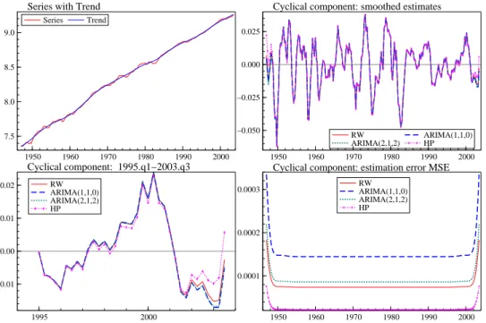
We consider now the trend-cycle decomposition with cutoff frequency ωc = 0.16
cor-responding to a period of about 10 years (39.7 quarters) and λ = 1600; each ARIMA model implies a different representation for the components; estimates of the latter, com-puted by the Kalman filter and smoother for the corresponding state space model, are displayed in figure 3, where the trend component refers to the ARIMA(2,1,2) model. The HP cyclical component is also displayed in the second and the third panel, which
presents ˜ψt|T for the last years in the sample, in order to appreciate better the differences
among the estimates. The HP cycle is the MMSLE of the cycle under the IMA(2,2) model
∆2y
t = (1 − 1.7771L + 0.7994L2)ξt, which would not be selected for the series under
investigation, being manifestly misspecified.
As figure 3 shows the HP estimates at the end of the sample differ from those that would be obtained from the model based decompositions. The optimal filter varies with the times series model for yt; however, the estimates for the ARIMA(1,1,0) and ARIMA(2,1,2)
are indistinguishable, and those for the RW model are quite close. Differences arise with respect to the estimation MSE, plotted in the last panel. That arising from the HP filter is a clear underestimation of the MSE that would arise from models that provide a better representation of the series. We notice also that the latter is quite sensitive to the model selected, being greater for the ARIMA(1,1,0) model.
Leaving the other parameters unchanged (m = 2 and n = 0), we next consider the model-based filter that arise for the cutoff frequency equal to 1.26, corresponding to a period of 5 quarters and λ = 0.52.
This filter has been adopted by Artis, Marcellino and Proietti (2004) in order to extract a lowpass component reducing the amplitude of those fluctuations with periodicity less than the minimum cycle duration (one year and a quarter), which is employed used to date the peaks and troughs of the business cycle; as a matter of fact, in dating the business cycle, we should abstract from those high frequency movements that cannot qualify as cyclical because they are too short lived.
The estimates of the components and the estimation error MSE are presented in figure 4. Given the properties of the series under investigation (the high frequency components of ∆ythave little amplitude), the estimates of the highpass component do not vary with
difference pertains the MSE, which in turn is very small and close to zero. This reflects the fact that for an integrated series, components with high cutoff frequency are estimated with greater reliability.
The example fosters the conclusions that long run trends are estimated less reliably than short run ones. We notice in closing that both cyclical components are affected by a change in volatility, as documented in Stock and Watson (2002).
5.2
The ARIMA(1,1,0) case
The magnitude of the revision process is assessed comparing the final estimation error MSE with the real time one.
Since the MSE of the filtered and smoothed estimates is identical for the two com-ponents (recalling µt− ˜µt|t = ˜ψt|t− ψt), let us concentrate on the cycle and denote the
variance of the real time and final estimates respectively by Var(ψt|Yt) and Var(ψt|Y∞),
where Yt is the semi-infinite sample {. . . , yt−1, yt} and Yt∞ is the doubly-infinite
sam-ple {. . . , yt−1, yt, yt+1, . . .}. The variance of the filtered estimates admits the following
decomposition:
Var(ψt|Yt) = Var(ψt|Y∞) + VR,
where VR= E[( ˜ψt− ˜ψt|t)2] is the revision error variance. Thus the ratio
R = Var(ψt|Yt))
Var(ψt|Y∞)
= 1 + VR
Var(ψt|Y∞)
, (9)
measures the relative importance of the revision process; R moves away from unity, which is the reference value that would be achieved were the components fully estimated in real time, as the variance of the revisions increases relative to the real time estimation error
The ratio (9) clearly depends on the ARIMA model for yt; in this paper we limit the
analysis of its behaviour to the fairly realistic and representative case when the series fol-lows the ARIMA(1,1,0) process (1 − φL)(∆yt− c) = ξt. If φ is positive, the dynamics of ∆ytare dominated by low frequency components and viceversa; we mention that similar results hold for the ARIMA(0,1,1) process. Figure 5 displays the values of R against the cutoff frequency for different combinations of the pair m, n. Both the numerator and the denominator are evaluated by the steady state Kalman filter and smoother for the state space representation given in the appendix.
The main evidence can be summarised as follows:
• For a given φ, ωcand m = 1, 2, increasing n enhances the relative magnitude of the
revision process.
• In the RW case (φ = 0) we have the interesting property that choosing n = m
makes R invariant to the cutoff frequency.
• For given φ, ωc and n, the magnitude of the revision process increases with m.
Hence the choice of a more flexible trend results cœteris paribus in larger revisions.
• Long run trends (ωcis low) are subject to comparatively smaller revisions if ∆ytis
dominated by low frequencies fluctuations (φ > 0).
6
The Model Based Interpretation of Bandpass Filters
A popular approach to the measurement of the business cycle entails selecting all the fluctuations with a specified range of periodicities, namely those ranging from one and a half to eight years. If s denotes the number of observations in a year, the fluctuations with
periodicity between 1.5s observations (e.g. 6 quarters, or 18 months) and 8s observations (e.g. 32 quarters or 96 months) are included.
Given the two cutoff frequencies, ω1c = 2π/(8s) and ω2c = 2π/(1.5s), the ideal
bandpass filter has unit gain inside inside the interval [ω1c, ω2c] and zero outside.
This approach has been popularized by Baxter and King (1999), who propose a 3s-terms approximation to the ideal filter; Christiano and Fitzgerald (2003) investigated the problem of finding the optimal linear approximation of the ideal filter, given a particular parametric model. They end up suggesting that for macroeconomic time series the filter derived assuming a random walk model for ytis suitable.
In this section we consider bandpass filters constructed from the principle of decom-posing the lowpass component in (6). Let us consider fixed values of m and n and two cutoff frequencies, ω1c and ω2c > ω1c, with corresponding values of the smoothness
pa-rameter λ1and λ2, determined according to (3). Obviously λ1 > λ2.
The trend-cycle decomposition corresponding to the triple m, n, λ2 (or, equivalently,
m, n, ω2c), is as in (6): yt = µ2t+ ψ2t, ∆dµ 2t = c +(1+L) n ϕ2(L) θ(L) φ(L)ζ2t, ζ2t ∼ NID(0, σ2) ψ2t = (1−L) m ϕ2(L) θ(L) ∆dφ(L)κ2t, κ2t∼ NID(0, λ2σ2) (10) with |ϕ2(L)|2 = |1 + L|2n+ λ2|1 − L|2m.
We can similarly define the trend-cycle decomposition corresponding to the triple
m, n, λ1 (or, equivalently, m, n, ω1c), yt = µ1t + ψ1t. As λ1 > λ2 this decomposition
features a lower cutoff frequency, ω1, thereby yielding a smoother trend. The components
µ1tand ψ1tare defined as in (10), with ϕ1(L), ζ1t ∼ NID(0, σ2) and κ1t ∼ NID(0, λ1σ2)
|1 + L|2n+ λ
1|1 − L|2m.
The lowpass component µ2t can in turn be decomposed using the orthogonal
decom-position of the disturbance ζ2t:
ζ2t = ϕ2(L) ϕ1(L) ζ1t+ (1 − L)m ϕ1(L) κ1t (11) with ζ1t∼ NID(0, σ2), κ1t ∼ NID ³ 0, (λ1− λ2)σ2 ´ , E(ζ1jκ1t) = 0, ∀j, t.
Under this setting, the ACGF of both sides of (11) is constant and equal to σ2.
Replacing (11) into (10) and writing µ2t = µ1t+ ψ1t∗, enables ytto be decomposed in
three components, representing the lowpass, bandpass and highpass components, respec-tively. yt = µ1t+ ψ∗1t+ ψ2t, ∆dµ 1t = c +(1+L) n ϕ1(L) θ(L) φ(L)ζ1t, ζ1t∼ NID(0, σ2) ψ∗ 1t = (1+L) n(1−L)m ϕ1(L)ϕ2(L) θ(L) ∆dφ(L)κ1t, κ1t ∼ NID (0, (λ1− λ2)σ2)) (12)
and ψ2tis the highpass component of the decomposition (10).
The decomposition can be cast in state space form and the components estimated using the Kalman filter; the latter automatically projects the bandpass filter onto the available sample, without the need to resort to forecast extensions or analytic derivation of the weights, and also provides the reliability measures, conditional on the ARIMA model for the series and its parameters.
As far as US GDP is concerned, figure (6) displays the smoothed estimates of the bandpass component, E(ψ1t∗|YT), conditional on the estimated ARIMA(1,1,0) model, and
Es-sentially, the bandpass cycle is a smoothed version of the latter, devoid of high frequency fluctuations. The last panel shows that the bandpass is characterised by a higher estima-tion error variance in the central porestima-tion of the sample with respect to the highpass, but the situation is reversed at the extremes of the sample. We shall return to this issue shortly.
Given the availability of a doubly infinite sample, the Wiener-Kolmogorov estimator of the bandpass component is
˜ ψ∗ 1t = wψ∗ 1(L)yt, wψ∗1(L) = |1 + L|2n|1 − L|2m |ϕ1(L)|2|ϕ2(L)|2 (λ1 − λ2).
The gain of the filter for two combinations is plotted in the first panel of figure 6, which reports also that of the BK filter for comparison.
There are two interesting things to notice: first, denoting by wµi(L) and wψi(L), i =
1, 2, the WK filters for extraction of µit and ψit, respectively, (11) implies wψ∗
1(L) =
wµ2(L) − wµ1(L) = wψ1(L) − wψ2(L), and thus the bandpass filter is obtained as the
contrast between two lowpass or highpass filters defined at different cutoffs. The second implication of (11) is that wψ∗
1(L) = wψ1(L)wµ2(L)(λ2 − λ1)/λ1, which
enables the interpretation of the historical bandpass filter as a cascade filter, such that the highpass filter defined at the cutoff ω2c is applied to the estimate of the lowpass (trend)
component defined at the cutoff ω1c, rescaled by the factor (λ2− λ1)/λ1.
We now turn our attention to the comparison of the final estimation error variances con-cerning the bandpass and highpass components, ψ∗1tand ψ1t. Using the standard
Wiener-Kolmogorov expressions for these variances, it is immediate to determine the following bounds for the efficiency of the bandpass estimates:
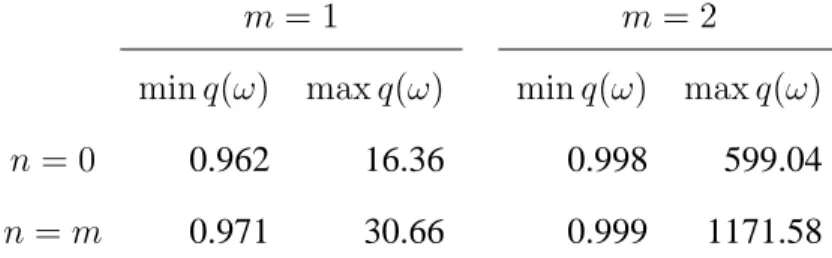
min q(ω) ≤ Var(ψ∗1t|Y∞) Var(ψ1t|Y∞) = Rπ 0 ge1(ω)q(ω)dω Rπ 0 ge1(ω)dω ≤ max q(ω)
where ge1(ω) is the spectral generating function of the final estimation error ψ1t− ˜ψ1t, see
section 4, and q(ω) is the Fourier transform of
q(L) = λ1− λ2 λ1 Ã |ϕ1(L)ϕ2(L)|2− (λ1− λ2)|1 + L|2n|1 − L|2m |ϕ2(L)|4 ! .
For the leading case of interest, that is ω1c = 2π/(8s) and ω2c= 2π/(1.5s), the minima
and maxima arising for some values of m and n are reported in the table below:
m = 1 m = 2
min q(ω) max q(ω) min q(ω) max q(ω)
n = 0 0.962 16.36 0.998 599.04
n = m 0.971 30.66 0.999 1171.58
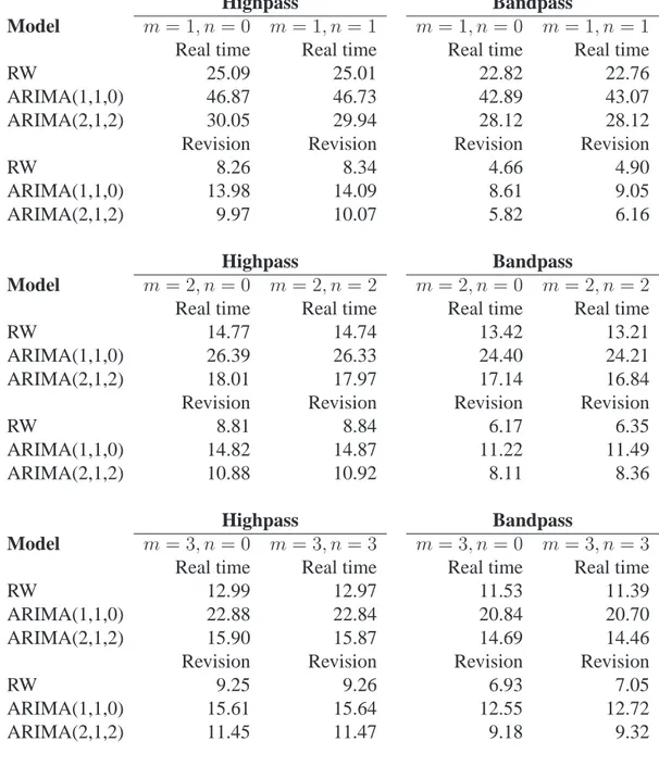
These bounds entail that the variance ratio is likely to be greater than one, so it can be concluded that the final estimation error uncertainty is greater for the bandpass estimates. As far as the trade-off between the estimation error reliability and revisions is con-cerned, there is no sharp theoretical result available, since it is specific to the ARIMA model for the series. Therefore, we illustrate the main findings with respect to US GDP. Table 1 reports the real time estimation error variance and revision error variance for high-pass and bandhigh-pass cyclical components extracted from US GDP, using 3 ARIMA models and the usual cutoffs ω1c = π/16 and ω2c = π/3
The trade-off is essentially the same for the bandpass component as that for the high-pass one: the estimation error variance of the real time (and the historical - given in the table by the difference between the real time and revision error variance) estimates de-creases with m, n, but the variance of the revision inde-creases. Thus the usual trade-off has to be faced. The choice of m, n which for given cutoffs minimises the variance of the revisions also maximises the size of the estimation error.
It might be though that for the design of the bandpass filter, involving the choice of the parameters m and n given the cutoffs, one should adopt the criterion of minimising the real time error variance Var(ψ1t∗|Yt), the latter representing a compromise of two elements of reliability, namely the sum of Var(ψ1t∗|Y∞) and VR; this is illusory, however, as the variance of the theoretical component ψ∗1talso varies with m and n.
It is clear from the table that both Var(ψ∗1t|Yt) and Var(ψ1t|Yt) decreases
monotoni-cally with both m and n; the computations can be extended for higher values of the two parameters, confirming that these quantities decrease at an ever smaller rate, until the computations break down due to numerical instability.
The table also highlights a reduction in both the real time and revision error variance as we move from the highpass to the bandpass; however, the latter is more substantial so that the final estimation error variance increases (this is reflected also in the last panel of figure 6).
As a consequence, it cannot be concluded that the bandpass is preferable to the high-pass component.
7
Conclusions
The paper has focused on a class of trend-cycle filters that is optimal for a particular local trend model and that depends on the order of integration of the trend (trend flexibility), on the order of the unit root at the Nyquist frequency (trend smoothness), and the relative variance of the cyclical component. The trend filter can be characterised as a lowpass filter whose cutoff frequency depends on the three parameters.
By embedding the trend-cycle decomposition within the ARIMA time series model for a univariate time series we provide a model-based framework that enables inferences on
the unobserved components to be conducted by means of the Kalman filter and smoother associated to the relevant state space model. The components select certain features of the series and in this respect they represent an artificial construct. Nevertheless, the model-based interpretation allows to formalise the discussion on the relevant issue of the uncer-tainty by which certain signals or components are estimated.
In particular, it has been shown that for the type of nonstationary time series usually encountered in macroeconomics more stable components and long run trends and cycles, characterised by lower cutoff frequencies are estimated with less reliability. Moreover, in designing the filter the analyst faces some trade-offs. The purpose of this paper was that of illustrating them. In particular, if on the hand increasing the flexibility of the trend and its smoothness via the introduction on noninvertible MA features for a given cutoff frequency enhances the reliability of the signal, in real time the signal will be subject to larger revisions.
Smoothness priors have their costs, as the quest for smooth signals results in larger revisions and greater discrepancies between real time and final estimates. This ties in well with the intuition that, the smoother the trend, the more observations are needed before the estimate settles down to its final value, and thus the greater the amount of revision involved.
Finally, the bandpass component provides a cleaner signal with respect to the highpass cycle; nevertheless, it is not necessarily superior in terms of its reliability, since it is characterised by an higher final estimation error variance.
References
Ansley, C.F., Kohn, R., 1985. Estimation, filtering and smoothing in state space models with incompletely specified initial conditions. The Annals of Statistics, 13, 1286-1316.
Artis, M., Marcellino, M., Proietti, T., 2004. Dating Business Cycles: a Methodological Contribution with an Application to the Euro Area. Oxford Bulletin of Economics and
Statistics, 66, 537–574.
Baxter, M., King, R.G., 1999. Measuring Business Cycles: Approximate Band-Pass Fil-ters for Economic Time Series. The Review of Economics and Statistics, 81, 575–593.
Burridge, P., Wallis, K.F., 1988. Prediction theory for autoregressive-moving average pro-cesses. Econometric Reviews, 7, 65–9.
Christiano, L.J., Fitzgerald, T.J., 2003. The band pass filter. International Economic
Re-view, 44, 435–465.
de Jong, P., 1989. Smoothing and interpolation with the state space model. Journal of the
American Statistical Association, 84, 1085–1088.
de Jong, P., 1991. The diffuse Kalman filter. Annals of Statistics, 19, 1073–83.
Doornik, J.A., 2001. Ox. An Object-Oriented Matrix Programming Language. Timber-lake Consultants Press, London.
G´omez, V., 2001, The Use of Butterworth Filters for Trend and Cycle Estimation in Eco-nomic Time Series. Journal of Business and EcoEco-nomic Statistics, 19, 365–373.
Hodrick J.R. and Prescott E.C., 1997. Postwar U.S. business cycles: an empirical investi-gation, Journal of Money, Credit and Banking, 29, 1–16.
Harvey, A.C., 1989. Forecasting, Structural Time Series and the Kalman Filter, Cam-bridge University Press, CamCam-bridge.
Harvey, A.C., and J¨ager, A., 1993. Detrending, stylized facts and the business cycle.
Journal of Applied Econometrics, 8, 231-247.
Kaiser, R. Maravall A., 2001. Measuring Business Cycles in Economic Time Series, Lec-ture Notes in Statistics, 154, Springer-Verlag, New York.
Koopman, S.J., 1997. Exact initial Kalman filter and smoother for non-stationary time series models. Journal of the American Statistical Association 92: 1630–8.
Koopman, S.J., Shephard, N., Doornik, J.A., 1999. Statistical algorithms for models in state space using SsfPack 2.2. Econometrics Journal, 2, 113–66.
Ng, C.N., Young P.C., 1990, Recursive estimation and forecasting of non-stationary time series. Journal of Forecasting, 9, 173-204.
Morley, J.C., Nelson, C.R., Zivot, E., 2002. Why are Beveridge-Nelson and Unobserved-Component Decompositions of GDP So Different? Review of Economics and Statistics, 85, 235–243.
Orphanides, A., van Norden, S., 2002. The Unreliability of Output Gap Estimates in Real Time. Review of Economics and Statistics, 84, 569–583.
Percival, D.B., and Walden, A.T., 1999. Wavelet Methods for Time Series Analysis, Cam-bridge Series in Statistical and Probabilistic Mathematics, CamCam-bridge University Press.
Pollock, D.S.G., 2000. Trend Estimation and De-trending via Rational Square-wave Fil-ters. Journal of Econometrics, 99, 317–334.
Sayed, A.H., and Kailath, T., 2001. A Survey of Spectral Factorization Methods.
Numer-ical Linear Algebra with Applications, 8, 467–496.
Stock J.H., and Watson, M., 2002. Has the business cycle Changed and Why? NBER
Working Paper No. w9127.
Whittle P., 1983. Prediction and Regulation by Linear Least Squares Methods, Second edition. Basil Blackwell, Oxford.
Table 1: Real time estimation error variance and revision error variance (multiplied by 105) for highpass and bandpass cyclical components extracted from US GDP, using 3
ARIMA models.
Highpass Bandpass
Model m = 1, n = 0 m = 1, n = 1 m = 1, n = 0 m = 1, n = 1
Real time Real time Real time Real time
RW 25.09 25.01 22.82 22.76
ARIMA(1,1,0) 46.87 46.73 42.89 43.07
ARIMA(2,1,2) 30.05 29.94 28.12 28.12
Revision Revision Revision Revision
RW 8.26 8.34 4.66 4.90
ARIMA(1,1,0) 13.98 14.09 8.61 9.05
ARIMA(2,1,2) 9.97 10.07 5.82 6.16
Highpass Bandpass
Model m = 2, n = 0 m = 2, n = 2 m = 2, n = 0 m = 2, n = 2
Real time Real time Real time Real time
RW 14.77 14.74 13.42 13.21
ARIMA(1,1,0) 26.39 26.33 24.40 24.21
ARIMA(2,1,2) 18.01 17.97 17.14 16.84
Revision Revision Revision Revision
RW 8.81 8.84 6.17 6.35
ARIMA(1,1,0) 14.82 14.87 11.22 11.49
ARIMA(2,1,2) 10.88 10.92 8.11 8.36
Highpass Bandpass
Model m = 3, n = 0 m = 3, n = 3 m = 3, n = 0 m = 3, n = 3
Real time Real time Real time Real time
RW 12.99 12.97 11.53 11.39
ARIMA(1,1,0) 22.88 22.84 20.84 20.70
ARIMA(2,1,2) 15.90 15.87 14.69 14.46
Revision Revision Revision Revision
RW 9.25 9.26 6.93 7.05
ARIMA(1,1,0) 15.61 15.64 12.55 12.72
A
State space representation
The spectral factorisation ϕ(L)ϕ(L−1) = a0+ a1(L + L−1) + · · · + ak
³ Lk+ L−k´, k = max(m, n) with aj = I(j ≤ n) 2n n + j + I(j ≤ m) 2m m + j ,
where I(·) is the indicator function, taking value 1 if the argument is true and 0 otherwise, can be achieved via the Riccati equation method presented in Sayed and Kailath (2001).
Let now φ(L)∗ denote the AR polynomial φ(L)∗ = φ(L)ϕ−10 ϕ(L) = 1 − φ∗1L −
· · · − φp+q∗Lp+q ∗
, common to the representation of the trend and the cycle in (6), and let
θµ(L) = (1 + L)nθ(L), the MA polynomial of the trend component. Further, define the
orders qµ = max(p + q∗, n + q + 1), qψ = max(p + q∗, q + 1).
The state space representation of (6) consists of the measurement equation yt = z0αt,
with z0 =hz0 µ, z0ψ i , αt= [α0µ,t, α0ψ,t]0, z0µ= [i0d+1, 00qµ], z 0 ψ = [1, 00qψ];
and the transition equation αt+1 = Tαt+ c + R²twith ²t= ϕ−1/20 [ηt, κt]0,
T = diag(Tµ, Tψ), c = [cz0µ, 00]0, R = diag(θµ, θψ), Tµ = A B 0 T∗µ ,
where A is a d × d upper triangular matrix with elements aij = 1, j ≥ i, and aij = 0, B is d × qµ matrix with zero elements except for the first column, which contains unit
elements, B = [id, 0], and T∗ µ= φ∗µ Iqµ−1 00 , Tψ = φ∗ψ Iqψ−1 00 , θµ= [1, θµ,1, θµ,2, . . . , θµ,qµ]0, θψ = [1, θψ,1, θψ,2, . . . , θψ,qψ]0, φ ∗ µ= [φ∗µ,1, φ∗µ,2, . . . , φ∗µ,qµ] 0, φ∗ψ = [φ∗ ψ,1, φ∗ψ,2, . . . , φ∗ψ,qψ]
0. The nonzero AR coefficients in φ∗
µ and φ∗ψ are the
coeffi-cients of φ(L)∗, the nonzero MA coefficients in θµare those of the polynomial θµ(L), and
0.0 0.5 1.0 1.5 2.0 2.5 3.0 0.25 0.50 0.75 1.00 f(1,0, π /20) f(1,0, π /2) f(1,1, π /20) f(1,1, π /2) 0.0 0.5 1.0 1.5 2.0 2.5 3.0 0.25 0.50 0.75 1.00 f(2,0, π /20) f(2,0, π /2) f(2,2, π /20) f(2,2, π /2) 0.0 0.5 1.0 1.5 2.0 2.5 3.0 0.25 0.50 0.75 1.00 f(1,0, π /20) f(3,0, π /20) f(2,0, π /2) f(2,0, π /20) f(1,0, π /2) f(3,0, π /2) 0.0 0.5 1.0 1.5 2.0 2.5 3.0 0.25 0.50 0.75 1.00 f(1,1, π /20) f(3,3, π /20) f(2,2, π /2) f(2,2, π /20) f(1,1, π /2) f(3,3, π /2) Figure 1: Gain function of v arious trend filters f (m, n, ωc ).
0 1 2 3 −12 −10 −8 −6 −4 −2
d
=0
d
=0
ω c ln ∫ v( ω ) 2 d ω f(1,0, ω c ) f(2,0, ω c ) f(2,2, ω c ) f(1,1, ω c ) f(2,1, ω c ) f(3,0, ω c ) 0 1 2 3 −10 −5 0 5 10 15d
=1
d
=1
ω c f(1,0, ω c ) f(2,0, ω c ) f(2,2, ωc ) f(1,1, ω c ) f(2,1, ω c ) f(3,0, ωc ) 0 1 2 3 −20 −10 0 10 20 30 40d
=2
ω c f(2,0, ω c ) f(2,2, ω c ) f(3,3, ωc ) f(2,1, ω c ) f(3,0, ω c ) f(4,0, ωc ) Figure 2: Plot of ln Rπ 0 v( ω ) 2 dω v ersus the cutof f frequenc y ωc .1950 1960 1970 1980 1990 2000 7.5
8.0 8.5 9.0
Series with Trend
Series Trend 1950 1960 1970 1980 1990 2000 −0.050 −0.025 0.000 0.025
Cyclical component: smoothed estimates
RW ARIMA(2,1,2) ARIMA(1,1,0) HP 1995 2000 −0.01 0.00 0.01 0.02 Cyclical component: 1995.q1−2003.q3 RW ARIMA(1,1,0) ARIMA(2,1,2) HP 1950 1960 1970 1980 1990 2000 0.0001 0.0002 0.0003
Cyclical component: estimation error MSE
RW ARIMA(1,1,0) ARIMA(2,1,2) HP
Figure 3: U.S. Gross Domestic Product, 1947.q1 - 2003.q3. Trend cycle decomposition with m = 2, n = 0 and 2π/ωc= 39.7 (λ = 1600) corresponding to the HP filter
1950 1960 1970 1980 1990 2000
7.5 8.0 8.5 9.0
Series with Trend
Series Trend 1950 1960 1970 1980 1990 2000 −0.010 −0.005 0.000 0.005
Cyclical component: smoothed estimates
RW ARIMA(1,1,0) ARIMA(2,1,2) HP 1995 2000 −0.002 0.000 0.002 Cyclical component: 1995.q1−2003.q3 RW ARIMA(2,1,2) ARIMA(1,1,0) HP 1950 1960 1970 1980 1990 2000 0.000010 0.000015 0.000020
Cyclical component: estimation error MSE
RW ARIMA(1,1,0) ARIMA(2,1,2) HP
Figure 4: U.S. Gross Domestic Product, 1947.q1 - 2003.q3. Trend cycle decomposition with m = 2, n = 0 and 2π/ω = 5 quarters (λ = 0.52)
0.0 0.5 1.0 1.5 2.0 2.5 3.0 1.25 1.50 1.75 2.00
m
=1,
n
=0
φ =0.9 φ=0.5 φ=0.0 φ=− 0.5 φ = − 0.9 0.0 0.5 1.0 1.5 2.0 2.5 3.0 1.25 1.50 1.75 2.00m
=1,
n
=1
φ =0.9 φ=− 0.5 φ =0.5 φ = − 0.9 φ =0.0 0.0 0.5 1.0 1.5 2.0 2.5 3.0 1.5 2.0 2.5 3.0 3.5m
=2,
n
=0
φ =0.9 φ=0.5 φ=0 φ=− 0.5 φ = − 0.9 0.0 0.5 1.0 1.5 2.0 2.5 3.0 1.5 2.0 2.5 3.0 3.5m
=2,
n
=2
φ =0.9 φ=0.0 φ=− 0.9 φ =0.5 φ=− 0.5 Figure 5: V ariance ratio of filtered and smoothed estimation errors for the ARIMA(1,1,0) model ∆ yt = φ ∆ yt− 1 + ξt v ersus cutof f frequenc y ωc for dif ferent v alues of m, n .0.0 0.5 1.0 1.5 2.0 2.5 3.0 0.25 0.50 0.75 1.00 Gain
Baxter and King Ideal Bandpass
m = n = 6 HP bandpass ( m =2, n =0) 1950 1960 1970 1980 1990 2000 −0.025 0.000 0.025
US GDP Baxter and King cycle and Bandpass comp.
Baxter King Bandpass
1950 1960 1970 1980 1990 2000 −0.050 −0.025 0.000 0.025
US GDP Bandpass and Highpass components
Bandpass Highpass 1950 1960 1970 1980 1990 2000
Estimation error variance
Bandpass Highpass 6: U.S. Gross Domestic Product, 1947.q1 -2003.q3. Bandpass and highpass components with m = 2, n = 0 and f frequencies ω1c = 2π /32 and ω2c = 2π /6