Essays on economics and demography

Testo completo

(1)UNIVERSITÀ DEGLI STUDI DI ROMA "TOR VERGATA" FACOLTA' DI ECONOMIA DOTTORATO DI RICERCA IN ECONOMIA INTERNAZIONALE. XXII. CICLO DEL CORSO DI DOTTORATO. Essays on Economics and Demography. Tilman Tacke. A.A. 2008/2009 Docente Guida/Tutor: Prof. Robert J. Waldmann Coordinatore: Prof. Giancarlo Marini.

(2) Essays on Economics and Demography Updated version of a doctoral thesis presented by. Tilman Tacke to the Department of Economics Università degli Studi di Roma "Tor Vergata" Supervisor: Prof. Robert J. Waldmann. June 2009. 1.

(3) Contents 1 Infant Mortality and Relative Income. 6. 1.1. Introduction . . . . . . . . . . . . . . . . . . . . . . . . . . . . . .. 7. 1.2. Income Distribution and Health . . . . . . . . . . . . . . . . . . .. 11. 1.2.1. Speci…cation . . . . . . . . . . . . . . . . . . . . . . . . .. 13. 1.2.2. Data . . . . . . . . . . . . . . . . . . . . . . . . . . . . . .. 15. Results . . . . . . . . . . . . . . . . . . . . . . . . . . . . . . . . .. 18. 1.3.1. OLS Regressions . . . . . . . . . . . . . . . . . . . . . . .. 18. 1.3.2. Robustness of Regression Estimates . . . . . . . . . . . .. 19. Possible Explanations . . . . . . . . . . . . . . . . . . . . . . . .. 24. 1.4.1. Relative Deprivation . . . . . . . . . . . . . . . . . . . . .. 27. 1.4.2. Public Policy . . . . . . . . . . . . . . . . . . . . . . . . .. 29. 1.3. 1.4. 1.5. Conclusion. . . . . . . . . . . . . . . . . . . . . . . . . . . . . . .. 2 The Relative E¢ ciency of Public and Private Health Care. 33 38. 2.1. Introduction . . . . . . . . . . . . . . . . . . . . . . . . . . . . . .. 39. 2.2. Methods and Empirical Results . . . . . . . . . . . . . . . . . . .. 40. 2.2.1. Estimating health care e¢ ciency . . . . . . . . . . . . . .. 40. 2.2.2. Basic results . . . . . . . . . . . . . . . . . . . . . . . . .. 42. 2.2.3. Interpretation . . . . . . . . . . . . . . . . . . . . . . . . .. 50. 2.3. Conclusion. . . . . . . . . . . . . . . . . . . . . . . . . . . . . . .. 60. 2.4. Appendix . . . . . . . . . . . . . . . . . . . . . . . . . . . . . . .. 63. 2.4.1. Data . . . . . . . . . . . . . . . . . . . . . . . . . . . . . .. 63. 2.4.2. Additional regression table . . . . . . . . . . . . . . . . .. 66. 2.

(4) Abstract Di¤erences in demographics between countries and over time are caused by many political, economic and cultural circumstances. This research analyzes two of these circumstances and their possible in‡uence on infant mortality. The infant mortality rate varies internationally between 3 and more than 150 deaths per thousand live births. Di¤erences in per capita income explain these variations to a large extent. Chapter one and two discuss how the distribution of per capita income and the source of health care expenditure, both independent from their absolute levels, might help to explain di¤erences in mortality between countries with the same level of per capita GDP. Chapter 1 indicates the relevancy of the share of national income concentrated among a country’s richest 20% for health outcomes of the lowest three quintiles of the income distribution independent of their personal absolute income. A comparison of 93 countries suggests that the income distance between an individual and the people the individual directly observes at work or in the neighborhood might not be the only form of relative deprivation, but that the distance to the wealthy might matter as well. The results are not caused by the distribution of absolute income: previous research has shown that the level of GDP per capita is the single most important determinant of health outcomes (see Prichett and Summers, 1996), which our results con…rm. The chapter discusses possible explanations for the link between income distribution and health outcomes. Suggestions for two explanations are found: public disinvestment in human capital in countries where income is unequally distributed and relative deprivation, i.e. social comparison resulting in stress, risk taking behavior, or unwise consumption expenditure. Chapter 2 investigates the relative e¢ ciency of public and private health care spending in reducing infant and child mortality using cross-national data for 163 countries. The analysis shows that an increase in public funds is both, signi…cantly correlated with lower mortality rates and signi…cantly more e¢ cient in reducing mortality than private health care expenditure. The results indicate that an increase in private health care expenditure might even be associated with higher, not lower, mortality. Although some of the estimated di¤erence in the e¢ ciency of public and private health care expenditure can be explained by geographies and socioeconomic factors, chapter 1 concludes that the indications for such di¤erence are robust.. 3.

(5) Given the comments from the PhD committee, both chapters will be subject to changes.. The author will be pleased to send on request (email to. tacke@economia.uniroma2.it) the most recent version of the chapters.. 4.

(6) Acknowledgements I am deeply grateful for the support and encouragement provided by my supervisor, Professor Robert J. Waldmann. His guidance and constructive suggestions have shaped my thesis for the better in many ways. It is probably di¢ cult to …nd another supervisor as instructive and at the same time entertaining as him, still less one who is available for gmail-chats about added-variable plots on Sunday afternoon. I would also like to thank my thesis committee Prof. Giovanni Andrea Cornia, Prof. Andrea Brandolini, and Prof. Giovanni Vecchi for their excellent comments during and after my …nale examination. I am sure that these comments will help to substantially improve the quality of my work. During the doctorate I was fortunate to …nd myself within an extremely encouraging environment. I want to thank the coordinator of the Ph.D. Programme, Professor Giancarlo Marini, for his support and advice. I am particularly grateful to him and Professor Pasquale Scaramozzino for providing me the opportunity to gain teaching experience from early on, and to Dott.ssa Michela Carnevali for giving me a great deal of help in my everyday life at Tor Vergata. I would also like to acknowledge Dott. Piergiuseppe Cossu’s help throughout the three years of the Ph.D. Programme, but especially at the …nal stage of my dissertation. I would like to show my gratitude to all the teaching sta¤ of the Department of Economics and Institutions as well as to Aldo Christian, Daniele, Oege, Gianluca, Melody and my other colleagues at the University of Rome. I would also like to thank my friends Frank, Maxim, and Khaled for providing me feedback to some of my papers and life in general. Finally, it is my pleasure to thank those who I enjoy the most spending my time with, my parents Uta and Maurus, my brothers Moritz, Leo, and Fritz, my sister Clara, and my girlfriend Laura.. 5.

(7) Chapter 1. Infant Mortality and Relative Income Do health outcomes depend on relative income as well as on an individual’s absolute level of income? We use infant mortality as a health status indicator and …nd a signi…cant and positive link between infant mortality and income inequality using cross-national data for 93 countries. Holding constant the income of each of the three poorest quintiles of a country’s population, we …nd that an increase in the income of the upper 20% of the income distribution is associated with higher, not lower infant mortality. Our results are robust and not just caused by the concave relationship between income and health. The estimates imply a decrease in infant mortality by 1.5 percent for a one percentage point decrease in the income share of the richest quintile. The overall results are sensitive to public policy: public health care expenditure, educational outcomes, and access to basic sanitation and safe water can explain the inequality-health relationship. Our …ndings support the hypothesis of public disinvestment in human capital in countries with high income inequality. However, we are not able to determine whether public policy is a confounder or mediator of the relationship between income distribution and health. Relative deprivation caused by the income distance between an individual and the individual’s reference group is another possible explanation for a direct e¤ect from income inequality to health. Our results suggest two sorts of reference groups: an individual’s social peer group, visible at work or in the neighborhood, and the wealthy.. 6.

(8) 1.1. Introduction. Is income inequality associated with bad health outcomes? If so, what causes the relationship between distribution of income and health? This paper presents some new empirical evidence related to both questions. Even given the income of each of the three lowest income quintiles, we …nd a statistically signi…cant association of higher income inequality and worse health outcomes. Our …ndings support the relative income hypothesis, which asserts that the association between inequality and poor health outcome is not just due to absolute poverty. The results suggest that a one percentage point decrease in the income share of the highest quintile of the income distribution ("the rich") would be associated with a decrease in infant mortality by 1.5 percent. Given an estimated annual infant mortality of 5.86 million in the 93 countries covered (2000), the one percentage point reduction in the income share of the rich would prevent nearly 90,000 infant deaths each year. This estimated e¤ect does not require an increase in the absolute income of the poor as a result of income redistribution. We …nd evidence for public disinvestment in human capital in countries with high income inequality. The estimated link between inequality and health outcomes is sensitive to public health care expenditure, education outcomes and access to safe water and basic sanitation, but we have no ability to determine which are independent causes and which transmission channels. A further possible explanation for the income inequality-health relationship is relative deprivation: the distance in income between an individual and its reference group might a¤ect personal health outcomes. Most existing literature de…nes the neighborhood ("keeping up with the Joneses") as the reference group: low relative income compared to the local peer group may cause social stress and increase the probability of taking health risks such as smoking and alcohol consumption. We …nd suggestive evidence of an e¤ect of relative deprivation between similar social classes. However, our analysis indicates that the neighborhood might not be the only reference group that matters for health outcomes. We …nd a relative deprivation e¤ect also if we de…ne the top end of the income distribution as the reference group: controlling for the income of the poor, infant mortality is higher where the income distance between the poor and the rich is greater. Relative deprivation due to income distance to the rich may matter for health not because of stress or health risk taking, but if the non-rich try to emulate the consumption behavior of the rich by allocating a larger share of consumption from non visible goods (such as health care) to status goods. A direct e¤ect of income inequality on health outcomes is due to individuals’ absolute level of income (absolute income hypothesis). Suppose two countries 7.

(9) with identical average income per capita but di¤erences in income distribution. For a concave relationship between health and income - additional income has a smaller e¤ect on the health of rich people than on the health of poor people - we expect the unequal country to have worse average health outcomes. In addition to the absolute income hypothesis, the relative income hypothesis has been formulated to describe a further e¤ect of income distribution on health outcomes: the health of an individual might not only depend on the individual’s absolute income, but also on income compared to others in the same country. There are various theoretical rationales for the relative income hypothesis (for a discussion see Kawachi and Kennedy, 1999): income inequality may a¤ect health outcomes through (a) public disinvestment in human capital in countries with high income inequality, (b) reduced social cohesion, or (c) negative e¤ects of social comparison ("relative deprivation") such as increased stress, risk taking behavior, or unwise consumption. Also the link between inequality and health might not be due to a casual e¤ect of inequality on infant mortality, but due to omitted variable bias. The idea that relative poverty can cause absolute mortality is not new. It was noted by Adam Smith in The Wealth of Nations (1776). Smith argues that "necessaries" include "whatever the custom of the country renders it indecent for credible people to be without" and that such custom a¤ects the level of absolute poverty at which the population is stable due to insu¢ cient "ability of the inferior ranks of people to bring up families". A large body of literature analyzes the relationship between income distribution and health outcomes with controversial results (for a comprehensive review of existing literature see Wilkinson and Pickett (2006)). Wilkinson (1992) shows an association between high infant mortality and high income inequality for industrialized countries both in levels and over time. Waldmann (1992) uses data for 57 countries in the 1960s and 1970s and derives similar results. Marmot and Bobak (2000) show higher mortality rates as income inequality increases in Eastern Europe and the former Soviet Union. De Volgi et al. (2005) …nd support for a link between higher income inequality and lower life expectancy in Italy (1995-2000) and in 21 industrialized countries (2001). Some research …nds statistically signi…cant and adverse associations of income inequality and infant mortality that become statistically insigni…cant when controls are added: Judge et al.’s (1998) association does not remain statistically signi…cant when they control for female labor participation, Lynch et al.’s (2001) …ndings are largely driven by the United States. Other studies fail to …nd a statistically signi…cant relationship between income distribution and health outcomes: Gerdtham and. 8.

(10) Johannesson (2004) cannot …nd a statistically negative e¤ect from income inequality on infant mortality within Swedish counties or municipalities; Mellor and Milyo (2001, 2002) …nd no support for Wilkinson’s (1992) results; Wildman et al. (2003) replicate Waldmann’s (1992) model with more recent data, but are not able to achieve similar results. Two general patterns can be observed when comparing results from existing research: …rst, the aggregation level of the reference group matters, positive …ndings are usually found when income inequality is measured in larger areas (e.g. Mellor and Milyo, 2002; Soobader et al., 1999; Wilkinson and Pickett, 2006); second, the relationship between health and income distribution in international comparisons was temporarily lost during the decade after the mid-1980s (e.g. Mellor and Milyo, 2001; Wildman et al., 2003; Wilkinson and Pickett, 2006). Time-series analysis seems therefore di¢ cult: if the relationship between health and income distribution disappeared in the mid-1980s, we cannot describe this relationship with a constant coe¢ cient. Furthermore, a within estimator of the relationship between health and income inequality within countries over time would require assumptions concerning a time-lag between changes in the distribution of income and their possible e¤ects on health outcomes. To anticipate problems related to time-series analysis and low levels of aggregation we investigate the link between income distribution and health outcomes using an international cross-section analysis. Existing research questions the robustness and reliability of …ndings concerning the relative income hypothesis from international cross-section analysis mainly for two reasons: data quality and the aggregation problems. The comparability of international data describing income distributions is limited due to varying de…nitions of inequality and measurement problems (see Atkinson and Brandolini (2001) for a discussion of pitfalls in the use of income distribution data). Gravelle (1998) and Wildman et al. (2003) discuss the aggregation problem in aggregated level studies of the relative income hypothesis: when aggregated data is used, it is di¢ cult to distinguish between the absolute and the relative income hypotheses. The concave relationship between health and income could cause such aggregation problem. If the bene…t of one additional Dollar spent on health care is higher for the poor (e.g. spent for vaccination) than for the rich (e.g. spent for whitening of teeth), we would expect average health of a society to be lower in a more unequal country not because of adverse e¤ects of a lower relative income, but because of a lower absolute income of the poor. Many aggregate cross-section studies are subject to such aggregation problems (Wildman et al., 2003). Some authors suggest not using aggregated. 9.

(11) data for studies of income distribution and population health, but favor microdata instead. While this approach de…nitely solves the aggregation problem, it inevitably restricts the reference groups, which can be considered. If one uses micro data on health outcomes to study relative deprivation, it is necessary that reference group income is di¤erent for di¤erent families in the same micro data set. Wilkinson (1997) argues that health outcomes in deprived neighborhoods are poorer not because of the inequality within their neighborhoods, but compared to other neighborhoods. Such e¤ects might not be visible in studies of micro-data. Waldmann (1992) and Wildman et al. (2003) address the aggregation problem by using the income level of the poorest quintile and the income of the population between the twentieth and the ninety-…fth percentile to allow for the e¤ect of absolute income on health; they then test the relative income hypothesis by using the income share of the rich. Relative deprivation has been discussed as a possible explanation for the link between income inequality and health outcomes. The relative deprivation hypothesis assumes that the income distance between an individual and his or her reference group a¤ects the individual’s health. Reference groups are usually de…ned by individual characteristics and geographic coverage: Eibner and Evans (2005) for example de…ne the reference group as a combination of the state of residence, age, race, and education. Soobadera and LeClere (1999) investigate di¤erent levels of geographic aggregation of the reference group and …nd independent e¤ects of inequality on health at higher levels of aggregation. Deaton (2001) shows that mortality depends on income inequality within and between states. Runciman (1966) proposes two types of reference groups: individuals in the same neighborhood/social class and individuals serving as role models from higher social classes. Current literature focuses on relative deprivation between individuals from similar social classes resulting in health a¤ecting stress or risk taking behavior. Little attention has so far been given to the rich as a reference group for the non-rich and relative deprivation leading to unwise consumption. A further explanation for the health-inequality relationship is public investment in human capital. The idea is that countries with higher income inequality might spend less on public education or public health care. A reason for lower public investment might be that high income inequality leads to a divergence of the interest of the rich and the non-rich, with the rich trying to lobby for lower taxes and public services (Kawachi and Kennedy, 1999). Wilkinson and Pickett (2006) point to the di¢ culty to determine whether public investments are pathways or confounders of the relationship between income inequality and health outcomes.. 10.

(12) Given the contradictory results of earlier research and concerns regarding their design and data quality it seems worthwhile to reinvestigate the relationship between income distribution and infant mortality. The paper is divided into 5 sections. The section following the introduction discusses data, speci…cation, and estimation technique. The third section presents the results of the estimation and their robustness concerning subsample stability and choice of speci…cation. The fourth section discusses alternative justi…cations of the relationship between income distribution and health outcomes. The paper closes with a concluding section.. 1.2. Income Distribution and Health. Income is the single most important determinant of a country’s health status. People live longer and infant mortality is lower in rich countries than in poor countries (Prichett and Summers, 1996). The health-wealth relationship does not only hold among countries, but also within countries. While the income of a country increases over time, the health status improves accordingly, and at a moment in time wealthier people are healthier than their poorer fellow citizens (Deaton, 2003). Income distribution within a country might in‡uence average health outcomes in two ways: (a) the relationship between health and income is concave: an increase in income has a larger e¤ect on health among poor people than among rich people. The literature has referred to e¤ects of absolute income on health outcomes as the absolute income hypothesis; (b) holding constant an individual’s income, a more unequal distribution of income might reduce health because of, among many possible explanations, unwise expenditure or social stress. E¤ects of the relative income position on health outcomes have been described by the relative income hypothesis. In this chapter we discuss both hypotheses, starting with the e¤ect of income distribution via absolute levels of income. Table 1.1 shows Gini coe¢ cients as a proxy for income distribution, infant mortality as a health status indicator, and GDP per capita in purchasing power parity (PPP) for 125 countries in 1999-2003. Averages for the 25 countries with the highest Gini coe¢ cient are displayed at the left hand side, for the lowest Gini coe¢ cients at the right hand side. The table illustrates the association between higher infant mortality and both lower per capita income and higher income inequality. The most unequal countries are at the same time on average the poorest (average GDP per capita of $4,486) and have the highest infant mortality with 61 deaths per 1,000 live births. Infant mortality falls and av-. 11.

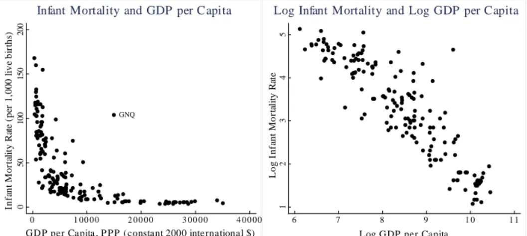
(13) erage income increases monotonically with more equal income distribution to 21 deaths per 1,000 live births and an average GDP per capita of $14,522 in countries with the lowest income inequality. Table 1.1: Infant Mortality and Per Capita Income, by Income Distribution Quintiles (1999-2003). Gini Infant Mortality Per Capita Income. Most unequal 25 countries. Second 25. Third 25. Fourth 25. Most equal 25 countries. 56 61 4,486. 46 59 4,490. 39 55 5,751. 34 29 12,005. 29 21 14,522. Notes: Infant mortality, per capita income ($, in PPP), and gini coe¢ cients are from World Bank’s World Development Indicators 2005.. The left graph in Figure 1.1 shows the concave relationship between income and health in an international comparison of 162 countries (mortality and income data for 1999-2003): infant mortality in countries with income per capita levels of $2,000 is on average 75 deaths per 1,000 live births; infant mortality decreases to (on average) approximately 12 deaths for income levels around $10,000; countries with an average income per capita around $25,000 have an infant mortality of on average 4 deaths per 1,000 live births. I.e., while infant mortality decreases on average by 8 deaths for a $1,000 increase in income in countries with a GDP per capita between $2,000 and $10,000, it decreases by 0.5 deaths for the same income increase in countries with a GDP per capita between $10,000 and $25,000. The right graph shows that the log of infant mortality of a country appears to be a linear function of the log of per capita GDP (in PPP) for the same country. We therefore use a log-log speci…cation in regressions of real income on infant mortality. In addition to an association of richer countries with better health outcomes, the absolute income hypothesis (Wildman et al., 2003) postulates, controlling for average income, a lower infant mortality in countries with low income inequality. To test the relationship between income distribution and infant mortality, we use di¤erent measures of average income as determinants of infant mortality. Using income distribution by quintiles we …nd that the explanatory power of average GDP per capita of the whole population is signi…cantly lower than the explanatory power of the average GDP per capita of the bottom 80% of the income distribution or of the lowest 60% of the income distribution. The highest explanatory power is associated with the third quintile: the median. 12.

(14) income seems to be more relevant for health outcomes then the average income. Table 1.2 shows these results based on income distribution and infant mortality data for 93 countries.1 ln(GDPq2. q4 ). denotes the log of the average GDP of the. second, plus the third, plus the forth quintile of the income distribution. These results support the use of median income (in Table 1.2 represented by the average income of the third quintile ln(GDPq3 )) as a proxy for social welfare. The regression of ln(GDPq3 ) yields the highest signi…cance and R2 in explaining international di¤erences in infant mortality.. 1.2.1. Speci…cation. This paper tries to overcome the aggregation problem and disentangle the relative from the absolute income hypothesis by using income data by quintiles. The advantage of using income per quintiles as opposed to average income of the whole population is that regression estimates for income per quintile capture the relationship between absolute income and infant mortality: infant mortality is expected to be higher in more unequal countries because the absolute income of the poor is lower. To isolate relative income e¤ects from absolute income e¤ects we introduce a measure of income distance between lower and upper quintiles. Holding constant the income of each of the three lower quintiles, the absolute income hypothesis predicts lower infant mortality for a larger distance between the income of lower and upper quintiles (as the larger income distance represents generalized Lorenz dominance). On the contrary, the relative income hypothesis would predict higher infant mortality associated with a larger income distance (as the larger income distance represents higher income inequality). Our empirical strategy to test the relative income hypothesis is very simple: we specify multivariate regressions that try to explain the level of infant mortality in 93 countries using the log of per capita GDP for each of the lower three quintiles and an explanatory variable. Inc representing the relative di¤erence. between the income of quintile i and quintile j.. ln(inf ant mortality) =. 1. +. ln(per capita GDPq1 ) + 3. 2. ln(per capita GDPq3 ) +. ln(per capita GDPq2 ) 4. Incqi;qj (1.1). Infant mortality is the number of deaths in the …rst year of life per thousand live births. We calculate. Inc as the di¤erence in income between two quintiles. relative to the income of the higher income quintile. E.g., for i = 1 and j = 4, 1 The. reduced sample size is due to the lack of data on income distribution by quintiles for. some countries.. 13.

(15) Figure 1.1: Infant Mortality and GDP per Capita (left), Log Infant Mortality and Log GDP per Capita (right). 4 3 1. 50. 100. GNQ. 2. Log Infant Mortality Rate. 150. 5. 200. Log Infant Mortality and Log GDP per Capita. 0. Infant Mortality Rate (per 1,000 live births). Infant Mortality and GDP per Capita. 0. 1 00 00. 2 00 00. 3 00 00. 4 00 00. 6. 7. GDP per Capita , P PP (constant 2000 international $). 8. 9. 10. 11. Log GDP per Capita. Table 1.2: Infant Mortality and Per Capita Income, OLS Estimates (1999-2005) ln(GDPq1. q5 ). ln(GDPq1. q4 ). ln(GDPq1. q3 ). ln(GDPq2. q4 ). (I). -0.87 (-22.37). (II). (III). (IV). -0.85 (-24.98) -0.83 (-24.96) -0.85 (-25.06). ln(GDPq3 ) Constant R2 N. (V). 10.58 (32.05) 0.84 93. 13.73 (32.61) 0.87 93. 13.13 (33.04) 0.87 93. 13.70 (32.74) 0.87 93. -0.85 (-25.10) 12.67 (33.61) 0.87 93. Dependent variable: log infant mortality; t-statistics in parentheses.. 14.

(16) Incq1;q4 denotes the di¤erence in income between the lowest quintile (q1) and the fourth quintile (q4) Incq1;q4 =. q4. q1 q4. (1.2). where q1 is the income share held by the bottom 20% of the income distribution. A value of. Incq1;q4 =. 2 3;. for example, indicates that the di¤erence between. the average income of a person in the lowest quintile and an average person in the fourth quintile amounts to 4. 2 3. of the average income of the wealthier people.. is not only an indicator for the validity of the relative income hypothesis,. but also for the absolute income hypothesis in upper quintiles. A positive. 4. is. evidence for the relative income hypothesis: the higher the distance between the average income levels of two quintiles, the higher the infant mortality. The other coe¢ cients should be positive. However, due to high multicollinearity between the …rst three variables, the estimates of their standard errors are large, so. 4. is the only coe¢ cient of interest. Our speci…cation allows to investigate the reference group that might matter for relative deprivation. Relative deprivation between individuals in similar social classes would be indicated by a positive and statistically signi…cant. 4. when we compare the income share of a quintile. with the share of the next higher income quintile (e.g. q3 with q4). Relative deprivation resulting from a comparison with the rich can be analyzed by using distant quintiles (e.g. q2 and q5) of the income distribution. We use further speci…cations to evaluate the relative income hypothesis. Similar to Waldmann (1992), we evaluate the relationship between infant mortality and the real income of the highest quintile or the income share of the highest quintile. The use of the real income of the highest quintile is problematic due to collinearity between the real incomes across quintiles.. 1.2.2. Data. To estimate equation (1.1) we collect data on 93 countries for the years 1999 to 2005.2 The aggregate population of these 93 countries is 87% of the world 2 The. countries included in the data set are: Albania, Armenia, Austria, Azerbaijan,. Bangladesh, Belarus, Belgium, Benin, Bolivia, Bosnia and Herzegovina, Brazil, Bulgaria, Burkina Faso, Cambodia, Cameroon, Canada, Chile, China, Colombia, Cote d’Ivoire, Croatia, Ecuador, Egypt, El Salvador, Estonia, Ethiopia, Finland, Georgia, Germany, Ghana, Guatemala, Guinea, Guyana, Haiti, Honduras, Hungary, India, Indonesia, Iran, Ireland, Israel, Italy, Jamaica, Jordan, Kazakhstan, Kyrgyz Republic, Lao PDR, Latvia, Lithuania, Luxembourg, Macedonia, Madagascar, Malawi, Mali, Mauritania, Mexico, Mongolia, Morocco, Mozambique, Nepal, Netherlands, Nicaragua, Nigeria, Norway, Pakistan, Panama, Paraguay, Philippines, Poland, Romania, Russian Federation, Senegal, Slovak Republic, Slovenia, South. 15.

(17) population. In the following we describe the construction of our data-set. The starting point is the UNU/WIDER World Income Inequality Database (WIID), version WIID2c (downloaded the 31st of July 2008). Compared to other secondary data-sets on income distribution the WIID o¤ers the advantage of including information about the coverage (area, population, ages), the de…nitions of income (consumption, expenditure, gross income, net income etc.), the income sharing unit (households, family, person etc.), the unit of analysis (indicating weighting of data with person or household weight), the equivalence scale used for weighting, and an assessment of data quality. Atkinson and Brandolini (2001) discuss problems of quality and consistency in income distribution data within and across countries. They demonstrate the dependency of regression estimates on the choice of income distribution data. To limit consistency and quality problems we select income distribution data by quintiles (in some cases calculated using data by deciles) only in case the whole population is covered across all age classes and including rural and urban areas (the WIID2c labels these speci…cations as "All" for the criteria area coverage (AreaCovr), population coverage (PopCovr), and age coverage (AgeCovrse)). We restrict the data to surveys that assign per capita household income to each member of the household (i.e. "Household" as the income sharing units (IncSharU), "Person" as the unit of analysis (UofAnala), and "Household per capita" as the equivalence scale (Equivsc)). To obtain a su¢ ciently large sample of countries we cannot restrict ourselves to one de…nition of income only. Observations include the distribution of consumption/expenditure, as well as of disposable income, disposable monetary income, and income without speci…cation of the treatment of taxes (from the Socio-Economic Database for Latin America and the Caribbean). In case there is more than one observation per country that satis…es our criteria, we prefer observations with a high quality ranking (WIID ranks the data quality from 1 to 3). Within a quality class we prefer consumption/expenditure data over disposable income data, and disposable income data over income data without speci…cation of tax treatment. For multiple observations of a country within a quality and de…nition class we try to collect data for the year 2000, in case there are no estimates for 2000, we use the estimate for the closest year to 2000 in the range 1999-2005. Out of the 93 observations, 56 use expenditure/consumption as the de…nition of income, 22 disposable income, 9 disposable monetary income, and 6 income without speciAfrica, Spain, Sri Lanka, Swaziland, Sweden, Tajikistan, Tanzania, Thailand, Tunisia, Turkey, Uganda, Ukraine, United Kingdom, United States, Uzbekistan, Venezuela, Vietnam, Yemen, and Zambia.. 16.

(18) …cation of the treatment of taxes. There are 39 observations of the year 2000, 12 for 1999, 20 for 2001, 9 for 2002, 8 for 2003, 3 for 2004, and 2 for 2005 in the data-set. To account for di¤erences in the income de…nition we introduce dummy variables. One dummy variable is constructed for each income de…nition. A shortcoming of the introduction of simple dummy variables for income de…nitions (e.g. the consumption dummy has the value of 1 for income distribution data based on consumption, otherwise a value 0) is that there is a selection bias: e.g. if all African countries use the same de…nition of income in their income distribution statistics, the dummy variable captures at the same time …xed e¤ects of di¤erences in the income de…nition and a …xed continent e¤ect for Africa. To overcome the selection bias, Deininger and Squire (1996) construct dummy variables comparing Gini coe¢ cients with di¤erent income de…nitions for the same country. Unfortunately only 20 out of the 93 countries in our data set provided income distribution data by quintiles (or deciles) with di¤erent de…nitions of income for the same year. We thus have to use simple dummy variables to account for de…nitional di¤erences: "Exp." for income distributions based on consumption/expenditure, "M. Inc." for disposable monetary income, and "NS Inc." income without speci…cation. Controlling for income de…nitions leads to substantial adjustments of our regression estimates, the dummy variable for data based on distribution of consumption/expenditure is always statistically signi…cant and positive. All regression estimates shown in this paper are therefore obtained using income de…nition dummy variables. Including a dummy variable for the year of the observation has almost no e¤ect on the estimates (changes of the point estimate are <2%, of its statistical signi…cance <1%). We therefore do not include a dummy for the year of the observation in our regressions. We use infant mortality as an indicator of health status as it is available for a large number of countries, and as it avoids potential problems of reverse causation associated with the relationship between adult health and income distribution (bad health outcomes cause income inequality). Unfortunately, de…nitions of infant mortality vary internationally; the comparability of infant mortality data is therefore limited. We therefore use child mortality (number of infants dying before reaching …ve years of age per 1,000 live births in a given year) as an additional variable. Our data for infant/child mortality and GDP per capita (in PPP, constant 2000 international $) is primarily provided by the World Bank’s World Development Indicators 2005 (CD version). Figures for infant mortality reported by the World Bank are often based on interpolations,. 17.

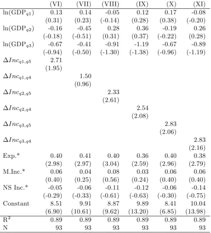
(19) extrapolations, or comparisons with other countries. However, the estimations are found to be reasonably accurate for cross-national comparisons at a point in time (Prichett and Summers, 1996). One observation of infant mortality (Canada) is taken from the Globalization–Health Nexus Database (Version 1). We use other variables as controls: public and private health care expenditure as a share of GDP, access to basic sanitation and safe water, and the ratio of total female enrollment in primary school to the female population of the age group are taken from the World Bank’s World Development Indicators 2005; obesity data (BMI>=30 kg/m2 , age group: 15-100 years) is provided by the World Health Organization for 2005; female literacy is taken from the UNESCO Institute for Statistics’Literacy and Adult Education Statistics Programme, if not available - which is the case for some OECD countries - from the CIA World Factbook 2007; female smoking prevalence (prevalence of current tobacco use among female adults (>=15 years) in 2005) is provided by the World Health Organization; HIV prevalence is taken from the World Bank’s World Development Indicators 2005, if not available from the UNAIDS’"2008 Report on the Global Aids Epidemic" (2001 estimates).. 1.3. Results. This section reports …rst the results of ordinary least squares (OLS) regressions corresponding to equation (1.1). We then discuss the robustness of the results concerning subsample stability and model speci…cation.. 1.3.1. OLS Regressions. Table 1.3 shows the results of estimating equation (1.1). The regression estimates support the validity of the relative income hypothesis as all (i.e. the coe¢ cients on. 4. coe¢ cients. Incqi;qj ) are positive and most of them statistically. signi…cant: holding constant the income of each of the lower three quintiles, a higher income of the upper two quintiles is associated with higher infant mortality. Note that the estimates for the income quintiles in Table 1.3 are imprecise due to multicollinearity as GDP per capita is a common factor used in the calculation of ln(GDPq1 ), ln(GDPq2 ), and ln(GDPq3 ). Multicollinearity does not bias coe¢ cient estimates, but causes large standard errors.3 3 We. calculate the variance in‡ation factor (VIF) to analyze potential problems arising from. multicollinearity. A large VIF indicates that it is di¢ cult to distinguish between the e¤ects of collinear variables. For a VIF of 10 or above, the estimated signi…cance of a variable is not trustworthy (Neter et al., 1996). In all regressions multicollinearity is a serious problem. 18.

(20) The average value of. Incq2;q5 in our sample is 75.5%: the average income. in the second poorest quintile of the population is therefore less than 25% of the average income in the riches income quintile. The results in (VIII) suggest that infant mortality increases with income inequality described by. Incq2;q5 with. semi-elasticity of 2.33 (t-statistic of 2.61). Holding the income share of the second poorest quintile constant at 10.8%, a one percentage point drop in the income share of the richest quintile from 46.5% to 45.5% would imply a decreased infant mortality of 1.5% in a country at the sample mean.4 If the same relationship were true for all countries in our sample, a one percentage point decline in the income share of the richest quintile in all 93 countries would avert annually nearly 90,000 deaths.5 This decrease would be due to e¤ects as postulated by the relative income hypothesis, not because of an increase in the absolute income of the lower quintiles. The other columns of Table 1.3 show that we …nd similar relationships between infant mortality and income distribution if we use the distance between either the highest or second highest quintile and any of the lower three quintiles. In the following we will use the distance between the second and the highest quintile of the income distribution as it achieves the statistically most stable results.. 1.3.2. Robustness of Regression Estimates. In this section we investigate the robustness of the results reported in Table 1.3 concerning the stability of our estimates with respect to in‡uential observations and model speci…cation. Controlling for outlying observations or leverage points and using di¤erent model speci…cations does not change our initial …nding: given the income of each of the three lower quintiles of the income distribution, an increase in the income of the higher quintiles is statistically signi…cantly associated with higher infant mortality. Regression estimates are sensitive to in‡uential observations, which can be divided into outliers and leverage points. Outliers are observations with large residuals: the value of the dependent variable is unusual given the values of its predictor variables; leverage points are observation with an extreme value on a among ln(GDP q1 ), ln(GDP q2 ), and ln(GDP q3 ) with VIFs always above 100. However, the collinearity between our measures of income distance and the other variables is low. All but one VIF (the VIF of the estimate for. 4. Incq1;q4 in regression (VII) equals 13.9, this might be the reason why. in (VII) is statistically not signi…cant) of our income distance measures are. below the critical threshold of 10. This implies that the signi…cance of the variables testing the relative income hypothesis is not overly sensitive to the inclusion of the other variables. 4 Note that the one percentage point decrease in the income share of the wealthiest quintile results in a decrease in Incq2;q5 from 75.5% to 74.9%. 5 The 93 countries reported 5.86 million child deaths in 2000.. 19.

(21) Table 1.3: Infant Mortality, Per Capita Income, and Income Distance, OLS Estimates (1999-2005) ln(GDPq1 ) ln(GDPq2 ) ln(GDPq3 ) Incq1;q5. (VI) 0.13 (0.31) -0.16 (-0.18) -0.67 (-0.94) 2.71 (1.95). (VII) 0.14 (0.23) -0.45 (-0.51) -0.41 (-0.50). (VIII) -0.05 (-0.14) 0.28 (0.31) -0.91 (-1.30). (IX) 0.12 (0.28) 0.36 (0.37) -1.19 (-1.38). (X) 0.17 (0.38) -0.19 (-0.22) -0.67 (-0.96). 1.50 (0.96). Incq1;q4. 2.33 (2.61). Incq2;q5. 2.54 (2.08). Incq2;q4. 2.83 (2.06). Incq3;q5 Incq3;q4 Exp.* M.Inc.* NS Inc.* Constant R2 N. (XI) -0.08 (-0.20) 0.26 (0.28) -0.89 (-1.19). 0.40 (2.98) 0.06 (0.40) -0.05 (-0.29) 8.51 (6.90) 0.89 93. 0.41 (2.97) 0.04 (0.25) -0.06 (-0.33) 9.91 (10.61) 0.89 93. 0.40 (3.04) 0.08 (0.56) -0.11 (-0.61) 8.87 (9.62) 0.89 93. 0.36 (2.59) 0.03 (0.24) -0.12 (-0.63) 9.89 (13.20) 0.89 93. 0.40 (2.96) 0.06 (0.40) -0.06 (-0.30) 8.41 (6.85) 0.89 93. 2.83 (2.16) 0.38 (2.79) 0.06 (0.40) -0.14 (-0.75) 10.04 (13.98) 0.89 93. Dependent variable: log infant mortality; t-statistics in parentheses. *Dummy variables for income distribution de…nitions.. 20.

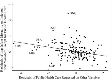
(22) predictor variable, i.e. leverage is a measure of how far an independent variable deviates from its mean. Figure 1.2 shows a partial scatter of infant mortality against the income distance between the second lowest and the highest income quintile. The residuals from a regression of the log of infant mortality on all explanatory variables except the income distance are plotted on the vertical axis, the residuals from a regression of the log of the income distance on all other variables are plotted on the horizontal axis. The slope of the line corresponds to the estimates of. 4. = 2:33 in regression (VIII) in Table 1.3. We de…ne an. outlier as an observation with a studentized residual, a type of standardized residual, exceeding +2 or -2.6 Two outlying observations are evident: Thailand (THA) with a studentized residual of -2.8 and Chile (CHL) with a studentized residual of -2.7. Further outlying observations include Swaziland (SWZ; studentized residual 2.3), Vietnam (VNM; -2.3), Spain (ESP; -2.1), Guinea (GIN; 2.1), Pakistan (PAK; 2.1), and Luxembourg (LUX; 2.0). The coe¢ cient on the income distance in regressions not including all eight outlying observations is 3.37 (compared to 2.61 in regressions including all observations) with a tstatistic of 4.56 (all observations: 2.61). By calculation of leverage values we can identify in‡uential observations. The following observations have leverage values exceeding (2k+2)/n, with k the number of independent variables: Brazil (BRA; leverage value of 0.20), Colombia (COL; 0.17), Haiti (HTI; 0.19), Honduras (HND; 019), Macedonia (MKD; 0.27), Netherlands (NLD; 0.18), Panama (PAN; 0.21), and Paraguay (PRY, 0.19). Excluding these observations we obtain a coe¢ cient on the income distance of 2.26 with a t-statistic of 2.39. Cook’s D can be used to detect in‡uential observations in general as it is a¤ected by large residuals and/or large leverage. Values exceeding 4/n indicate such in‡uential observations: Chile (CHL; 0.13), Thailand (THA; 0.09), Spain (ESP; 0.06), South Africa (ZAF 0.06), and Luxembourg (LUX; 0.05). Excluding these observations, the estimated coe¢ cient on the income distance becomes 3.18 with a t-statistic of 3.77. We use dummy variables for the countries identi…ed as in‡uential observations (using Cook’s D). If we include dummy variables for Chile, Thailand, Spain, South Africa, and Luxembourg into regression (VIII) all but South Africa and Luxembourg are statistically signi…cant: Thailand (t-statistic of -3.07), Chile (-2.86), Spain (-2.26), Luxembourg (1.96), and South Africa (1.37). For the rest of our analysis we therefore include dummy variables for Chile, Spain, 6A. studentized residual is calculated by division of a residual by its estimated standard. deviation. A studentized residual of +2 indicates that the observed value of an observation is 2 standard deviations above prediction.. 21.

(23) Figure 1.2: Partial Scatter of Infant Mortality against Income Distance between. Residual of Log Infant Mortality on Independent Variables Except for Income Distance -1 -.5 0 .5 1. Second Lowest and Highest Income Quintile. GIN PAK KAZ. MKD BIH. LUX. SWZ ZAF MEX. AZE IND CMR EGY TUR GUY USA LAO MLI CIV IRN IRL HT RUS I HUN BRA KHM GHAMAR BGD BFA MOZ MRT BEN ARM SVK NGA AUT IDN BEL GTSEN M NLD NOR UGA DEUGBR ZMB CAN TUN SLV UZB ETH VENCOL ROM MNG PRY BOL SVN LVA NIC FIN ISR HNDIT AJAM PHL POL EST MWI JOR BGR CHN ALB TJKPAN LTU UKR SWE MDG KGZ LKA TZA YEM ECUGEO BLR ESP HRV VNM THA. NPL. CHL. -.1 -.05 0 .05 .1 Residual of Income Distance Regressed on Other Variables. and Thailand, the exclusion leads to a larger and statistically more signi…cant relationship between infant mortality and income distribution: the estimated coe¢ cient on the income distance increases from 2.33 to 3.40, the t-statistic from 2.61 to 4.05 (see regression (XII) in Table 1.4).7 We investigate the general model speci…cation of equation (1). The set of explanatory variables in regression (XII) in Table 1.4 accounts for 92% of the variability in infant mortality between 93 countries. A computed F(10,81)=98.54 provides evidence that our basic set of predictor variables accounts for a statistically signi…cant amount of the variability in the model (p-value for > F = 0.000). The Shapiro-Wilk W test is designed to investigate whether errors are normally distributed. The computed W is 0.995, the p-value of 0.980 indicates that the assumption of normally distributed residuals cannot be rejected. In addition, a Cook-Weisberg test for heteroscedasticity (Cook and Weisberg, 1983) did not reject the null hypothesis of constant variance at any conventional signi…cance 7 Another. way to limit the in‡uence of outlying observations and leverage points on re-. gression estimates is to use robust regressions. Robust regressions con…rm our …ndings: the estimated coe¢ cient on the income distance is 2.93 with a t-statistic of 3.24.. 22.

(24) level (chi-square 2.04 with p-value of 0.154). The association between higher infant mortality and higher income inequality is not due to the chosen speci…cation (1.1). Table 1.4 shows the positive coe¢ cients on the income share of the highest quintile in regression (XIII) and on the log of real income of the highest quintile in regression (XIV). The results are statistically signi…cant with t-statistics of 3.90 and 3.92. Regressions (XV) and (XVI) include the log of real income of the fourth quintile, the association of higher infant mortality with higher income inequality remains statistically signi…cant. Regression (XVIII) has both a similar setup and similar …ndings to Waldmann (1992). Wildman et al. (2003) re-examine Waldmann’s investigations. One of Wildman et al.’s regressions is identical to regression (XVIII) but they …nd no statistically signi…cant partial correlation between the income share of the highest quintile and infant mortality. Note that the log of the aggregate real per capita income of the second, third, and fourth quintile (ln(GDPq2. q4 )). in regressions (XVII) and (XVIII) captures the association of. higher real absolute income and lower infant mortality, i.e support the absolute income hypothesis for these quintiles. The coe¢ cients on log real income of the poorer quintiles in all other regressions are statistically not signi…cant due to multicollinearity between ln(GDPq1 ), ln(GDPq2 ), and ln(GDPq3 ). By including the log of real per capita income of each of the three lower quintiles of the income distribution we control for the e¤ect of di¤erences in absolute income on infant mortality. However, using income by quintiles allows only to control for di¤erences between the income quintiles, not within quintiles. We include quadratic terms of the log of the real income of each of the lower three quintiles in the equation to correct for the curvilinear nature of the absolute income – infant mortality relationship. We would expect that the e¤ect of inequality due to curvature of the risk of infant mortality as a function of absolute income has implications for the estimated coe¢ cients on the real income of the lower quintiles, but not for the income distance. Regression (XIX) in Table 1.5 shows that our prediction is correct: the coe¢ cient on the income distance between the highest and the second lowest quintile remains unchanged. It also shows that the new variables are not statistically signi…cant and add very little to R2 : The reason is that we already use three or four parameters to correct for the curvilinear nature of the relationship between absolute income and infant mortality. Due to multicollinearity already the sign of the coe¢ cients on the real per capita income of the lower quintiles does not represent the relationship between higher absolute income and lower infant mortality. Adding more parameters based on the same raw numbers is thus very unlikely to improve the. 23.

(25) speci…cation. The quadratic terms are not included in the rest of our analysis.8 The de…nition of infant mortality varies internationally. We repeat our basic regression replacing infant mortality by child mortality (mortality before reaching …ve years of age) and "net child mortality" (mortality of children aged between 1 and 5 years of age).9 The income distance between the second and the highest quintile of the income distribution is in both cases statistically signi…cantly associated with higher child mortality. Our results support both, the relative and the absolute income hypothesis. The relationship between income and health of an individual is concave: higher individual income leads to better health but with a decreasing marginal e¤ect. High infant mortality in a country with high income inequality is not only due to low income of the poor: holding constant the absolute income of the poor, a higher distance to the income of upper quintiles is always associated with higher infant mortality. We have shown that the e¤ect can neither be explained with outlying observations, nor with our speci…cation or the de…nition of infant mortality.. 1.4. Possible Explanations. It is impossible to prove the existence of relative deprivation in data aggregated on country levels. Income distribution and infant mortality depend on many geographic, demographic, political, economic and cultural circumstances and we are not able to rule out that the association between income inequality and infant mortality is due to omitted variable bias. But even if we …nd controls that explain the relationship between health and income distribution, we do not know whether these factors are genuine confounders or pathways (see Wilkinson and Pickett, 2006). This section discusses indications for relative deprivation and the relevance of public policy for the link between income inequality and health. Although there is no obvious link between HIV and either the relative deprivation hypothesis or public policy, we add the prevalence of HIV as a control variable because it signi…cantly a¤ects our regression estimates. Column (B) in 8 The. RESET test (Regression Speci…cation Error Test) for right hand side variables can be. used to test the speci…cation of equation (1). The test tries to signi…cantly improve the model by including powers of the predictions of the model. The F-values of the RESET test for right hand side variables is 0.99 with a p-value of 0.47, well above the conventional signi…cance level of 0.05. The RESET test supports our log-log speci…cation. 9 The sample for regression (XXII) in Table 1.5 ("net child mortality") is reduced to 92 countries as Honduras reports identical numbers for infant and child mortality.. 24.

(26) Table 1.4: Di¤erent Speci…cations for Infant Mortality, Per Capita Income, and Income Distribution, OLS Estimates (1999-2005) (XII) 0.15 (0.44) 0.23 (0.28) -1.01 (-1.56). ln(GDPq1 ) ln(GDPq2 ) ln(GDPq3 ). (XIII) 0.06 (0.19) 0.08 (0.09) -0.77 (-1.24). (XIV) 0.03 (0.08) -0.17 (-0.21) -1.28 (-1.84). ln(GDPq4 ) ln(GDPq2. 3.40 (4.05). q5. 3.78 (3.39). Exp.* M. Inc.* NS Inc.* Chile** Spain** Thailand**. (XVII) 0.29 (1.19). (XVIII) 0.17 (0.77). -0.91 (-3.69) 3.66 (4.58). -0.80 (-3.43). 0.04 (3.90). ln(GDPq5 ). R2 N. (XVI) -0.03 (-0.08) -0.10 (-0.13) -0.99 (-1.04) -0.37 (-0.44). q4 ). Incq2;q5. Constant. (XV) 0.10 (0.27) 0.35 (0.41) -0.63 (-0.66) -0.43 (-0.52). 0.43 (3.54) 0.03 (0.20) -0.16 (-0.95) -0.98 (-2.92) -0.82 (-2.49) -1.06 (-3.26) 7.59 (8.75) 0.91 93. 0.49 (4.05) 0.07 (0.52) -0.24 (-1.45) -1.11 (-3.17) -0.81 (-2.44) -1.02 (-3.11) 8.41 (11.15) 0.91 93. 0.04 (4.47) 0.79 (3.92) 0.49 (4.07) 0.06 (0.49) -0.26 (-1.51) -1.11 (-3.19) -0.81 (-2.46) -1.02 (-3.12) 9.02 (13.24) 0.91 93. 0.44 (3.56) 0.03 (0.24) -0.14 (-0.84) -0.98 (-2.90) -0.82 (-2.49) -1.06 (-3.22) 7.41 (7.91) 0.91 93. 0.87 (3.24) 0.51 (4.04) 0.07 (0.54) -0.25 (-1.49) -1.12 (-3.19) -0.82 (-2.46) -1.01 (-3.07) 9.00 (13.12) 0.91 93. 0.41 (3.56) 0.01 (0.06) -0.11 (-0.70) -0.94 (-2.92) -0.85 (-2.64) -1.13 (-3.56) 8.50 (10.03) 0.92 93. Dependent variable: log infant mortality; t-statistics in parentheses. *Dummy variables for income distribution de…nitions. **Dummy variables for in‡uential observations.. 25. 0.48 (4.17) 0.06 (0.48) -0.21 (-1.29) -1.11 (-3.31) -0.83 (-2.57) -1.07 (-3.38) 9.24 (11.60) 0.92 93.

(27) Table 1.5: Further Speci…cations for Infant/Child Mortality, Per Capita Income, and Income Distribution, OLS Estimates (1999-2005) ln(GDPq1 ) ln(GDPq2 ) ln(GDPq3 ). (XIX) 0.15 (0.44) 0.23 (0.28) -1.01 (-1.56). (ln(GDPq1 ))2 (ln(GDPq2 ))2 (ln(GDPq3 ))2 Incq2;q5 Exp.* M. Inc.* NS Inc.* Chile** Spain** Thailand** Constant R2 N. 3.40 (4.05) 0.43 (3.54) 0.03 (0.20) -0.16 (-0.95) -0.98 (-2.92) -0.82 (-2.49) -1.06 (-3.26) 7.59 (8.75) 0.91 93. (XX) -0.03 (-0.01) 1.09 (0.14) -1.76 (-0.31) 0.01 (0.06) -0.04 (-0.11) 0.03 (0.13) 3.40 (3.88) 0.44 (3.16) 0.02 (0.17) -0.16 (-0.91) -0.98 (-2.83) -0.83 (-2.39) -1.06 (-3.17) 8.08 (2.14) 0.91 93. (XXI) 0.25 (0.64) 0.64 (0.69) -1.59 (-2.20). (XXII) 0.53 (0.84) 1.82 (1.19) -3.28 (-2.77). 4.10 (4.35) 0.42 (3.04) 0.11 (0.74) -0.21 (-1.15) -1.20 (-3.20) -0.74 (-2.02) -1.18 (-3.21) 8.40 (8.65) 0.91 93. 6.54 (4.18) 0.38 (1.68) 0.36 (1.51) -0.35 (-1.15) -2.11 (-3.43) -0.43 (-0.71) -1.86 (-3.09) 8.18 (5.03) 0.85 92. Dependent variable: log infant mortality (XIX), (XX); log child mortality (XXI); log net child mortality (XXII). t-statistics in parentheses. *Dummy variables for income distribution de…nitions. **Dummy variables for in‡uential observations.. 26.

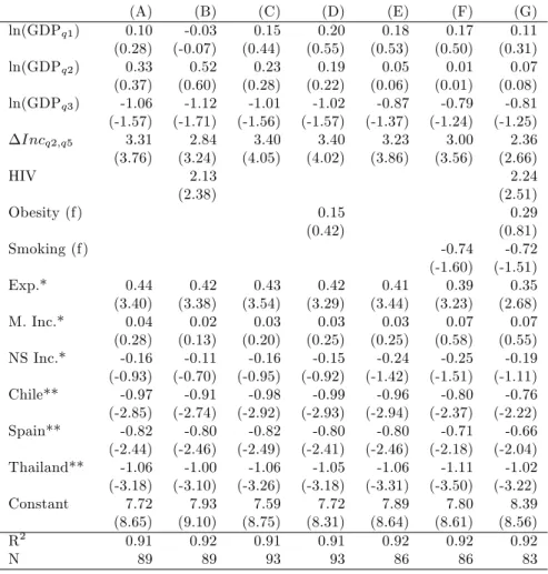
(28) Table 1.6 shows estimates for regressions including the real income of each of the lowest three quintiles, the income distance between the highest and the second lowest quintile, and the prevalence of HIV. Higher HIV prevalence is statistically signi…cantly partially correlated with higher infant mortality. The association between higher infant mortality and higher income distance decreases by 15% from 3:31 to 2:84, but remains statistically signi…cant with a t-statistic of 3:24.10. 1.4.1. Relative Deprivation. We use the common de…nition of relative deprivation as the di¤erence between an individual’s income and the income of his/her reference group (Jones and Wildman, 2008) and follow Runciman’s (1966) duality of reference groups: individuals in the same neighborhood/social class and individuals serving as role models from higher social classes. There is a large body of literature investigating relative deprivation within a social class and between similar social classes. Negative e¤ects of relative deprivation between and within social classes on heath are well documented. The Whitehall study (Marmot et al., 1984), e.g., …nds mortality di¤erences of British civil servants relative to their rank. Eibner and Evans (2005) use interview surveys to investigate relative deprivation and show, among other e¤ects, higher probabilities of death, and higher body mass index of relatively deprived individuals. The adverse e¤ects on individual health are usually explained by increased stress and risk taking behavior. However, relative deprivation in such sense does not fully explain our or Waldmann’s (1992) results. It seems unlikely that the income distance between individuals with very limited personal contact causes health a¤ecting stress or risk taking behavior. This might explain why existing research on relative deprivation usually neglects the top end of the income distribution as a possible reference group. However, our …ndings indicate that the income distance between individuals from distant social classes does matter for health outcomes. Our hypothesis is that, in addition to stress or health risk taking behavior of relatively deprived individuals, their consumption patterns might change depending on the concentration of income. Individuals might want to imitate the consumption patterns of high-income earners to increase their self-esteem. A high concentration of income at the top end of the income distribution leads to a visible divergence of consumption patterns between the rich and the non-rich. The non-rich might therefore increase their consumption of positional goods as 1 0 Note. that we have to compare results of regression (B) to regression (A). The speci…cation. of regression (A) is identical to regression (XIX) in Table 1.5, but the estimates di¤er slightly because of a reduced sample size (89 countries instead of 93).. 27.

(29) they wish to appear to be rich. Frank (2003) …nds a connection between higher expenditure for positional goods and higher income inequality. He argues that concerns about relative position lead to too much expenditure on positional goods and too little on nonpositional goods (Frank, 2005). A higher expenditure for positional goods implies a lower budget for nonpositional goods. Frank and Sunstein (2001) lists health care among these nonpositional goods. We are not able to directly test either of the hypotheses concerning the reference group underlying relative deprivation. However, our regression estimates support Runciman’s (1966) duality of reference groups: (a) we …nd indication for similar social classes as the reference group: the estimates for the income distance to the fourth quintile become statistically more signi…cant the closer the quintile of comparison. The distance between the lowest and the fourth quintile of the income distribution in Table 1.3 is not signi…cant (t-statistic of 0.96): the poor consider individuals in the fourth income quintile not to be their reference group. On the contrary the income distance to the fourth quintile becomes statistically signi…cant if compared with the second (t-statistic of 2.08) or third quintile (t-statistic of 2.16) of the income distribution; (b) in addition there are also indication for the rich as the reference group: the estimates for a link between higher infant mortality and higher income inequality are more signi…cant if we use comparisons of lower quintiles with the highest quintile, not with the fourth quintile. Table 1.3 shows that both, coe¢ cient and signi…cance of the income distance of each of the two lowest quintiles compared with the wealthiest quintile are higher than the same comparisons with the second wealthiest quintile. Our results suggest that both reference groups, similar social classes and the rich, matter for relative deprivation. Eibner and Evans (2005) show that relative deprivation a¤ects health via risky behavior such as increased smoking and poor eating or exercising habits. We use the prevalence of smoking among female adults, and female obesity as possible transmission channels of relative deprivation. Both variable are at the same time directly related to the risk of infant mortality. Regression (D) and (F) show estimations for the relationship between obesity/smoking and infant mortality in our data set. The results show no statistically signi…cant partial correlation between infant mortality and either obesity or smoking, nor do obesity or smoking explain the health-inequality relationship.11 We therefore 1 1 Our. results are surprising as the relationship between obesity/smoking and infant mortal-. ity is well documented in existing literature (e.g. Kleinman et al. (1988) relate 10% of infant deaths to maternal cigarette smoking; Chen et al. (2009) …nd an increased probability of neonatal death and overall infant death for obese women compared to normal weight woman of between 40% and 180%).. 28.

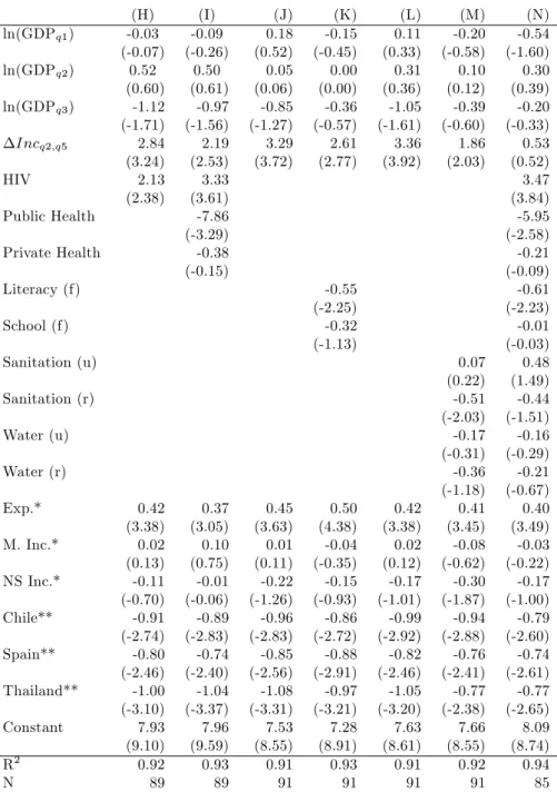
(30) fail to identify smoking or obesity as mediators of relative deprivation. Table 1.6: Infant Mortality, Per Capita Income, Income Distribution, HIV, and Risk Factors, OLS Estimates (1999-2005) ln(GDPq1 ) ln(GDPq2 ) ln(GDPq3 ) Incq2;q5. (A) 0.10 (0.28) 0.33 (0.37) -1.06 (-1.57) 3.31 (3.76). HIV. (B) -0.03 (-0.07) 0.52 (0.60) -1.12 (-1.71) 2.84 (3.24) 2.13 (2.38). (C) 0.15 (0.44) 0.23 (0.28) -1.01 (-1.56) 3.40 (4.05). Obesity (f). (D) 0.20 (0.55) 0.19 (0.22) -1.02 (-1.57) 3.40 (4.02). (E) 0.18 (0.53) 0.05 (0.06) -0.87 (-1.37) 3.23 (3.86). (F) 0.17 (0.50) 0.01 (0.01) -0.79 (-1.24) 3.00 (3.56). 0.41 (3.44) 0.03 (0.25) -0.24 (-1.42) -0.96 (-2.94) -0.80 (-2.46) -1.06 (-3.31) 7.89 (8.64) 0.92 86. -0.74 (-1.60) 0.39 (3.23) 0.07 (0.58) -0.25 (-1.51) -0.80 (-2.37) -0.71 (-2.18) -1.11 (-3.50) 7.80 (8.61) 0.92 86. 0.15 (0.42). Smoking (f) Exp.* M. Inc.* NS Inc.* Chile** Spain** Thailand** Constant R2 N. 0.44 (3.40) 0.04 (0.28) -0.16 (-0.93) -0.97 (-2.85) -0.82 (-2.44) -1.06 (-3.18) 7.72 (8.65) 0.91 89. 0.42 (3.38) 0.02 (0.13) -0.11 (-0.70) -0.91 (-2.74) -0.80 (-2.46) -1.00 (-3.10) 7.93 (9.10) 0.92 89. 0.43 (3.54) 0.03 (0.20) -0.16 (-0.95) -0.98 (-2.92) -0.82 (-2.49) -1.06 (-3.26) 7.59 (8.75) 0.91 93. 0.42 (3.29) 0.03 (0.25) -0.15 (-0.92) -0.99 (-2.93) -0.80 (-2.41) -1.05 (-3.18) 7.72 (8.31) 0.91 93. (G) 0.11 (0.31) 0.07 (0.08) -0.81 (-1.25) 2.36 (2.66) 2.24 (2.51) 0.29 (0.81) -0.72 (-1.51) 0.35 (2.68) 0.07 (0.55) -0.19 (-1.11) -0.76 (-2.22) -0.66 (-2.04) -1.02 (-3.22) 8.39 (8.56) 0.92 83. Dependent variable: log infant mortality; t-statistics in parentheses. *Dummy variables for income distribution de…nitions. **Dummy variables for in‡uential observations.. 1.4.2. Public Policy. Health outcome and income inequality will be a¤ected by public policy, which we allow for by including public health care expenditure, education outcomes, and access to basic sanitation and safe water in our regressions. Countries with a more egalitarian income distribution may at the same time have better public health care systems. The idea is that, rather than income inequality itself, di¤erences in the extent of and access to public health care 29.

(31) services cause the divergence of infant mortality. In countries with large differences between the income share of the lowest and the highest quintile of the income distribution, private expenditure on health care tends to be high and public expenditure tends to be low. Health care expenditure seems thus to be part to the link between income inequality and infant mortality: when we include the share of GDP that is privately and publicly spent for health care in our regression the association becomes statistically insigni…cant (regression (I) in Table 1.7). The coe¢ cient on the income distance between the richest and the poorest quintile decreases from 2.84 to 2.19, its t-statistic from 3.24 to 2.53. The estimate for the association of public health care expenditure and infant mortality is statistically signi…cant, negative, and large: -7.86 with a t-statistic of -3.29. The estimation implies an association of an increase in public health care expenditure of one percentage point of GDP with a decrease in infant mortality of nearly eight percent. On the contrary, private health care expenditure does not have a statistically signi…cant impact on infant mortality. These results indicate that the correlation between infant mortality and income inequality arises partly because income inequality is associated with low public expenditure and presumably limited access to health care for the poor. Public health care expenditure or access to health care services in general have already been used in attempts to explain the relationship between bad health outcomes and high income inequality. However, previous research has failed to explain such relation with cross-national di¤erences in private and public health care funding. Le Grand (1987) cannot …nd a statistically signi…cant relationship between public or private expenditure on medical care that could account for the relationship between inequality and health. Adda et al. (2003) provide indications that medical insurance coverage and access to medical services might not be the reason for a link between low socioeconomic status and bad health outcomes. Our …ndings suggest that di¤erences in health care expenditure can partially explain the association of income inequality and infant mortality. Education has often been found to have a strong e¤ect on infant mortality. Regression (K) shows the results of including female literacy and the ratio of total female enrollment in primary school to the female population of the age group into a regression of the log of average income by quintiles and income distance on the log of infant mortality. The inclusion of female literacy has the expected e¤ect: higher rates of female literacy are associated with lower infant mortality, the results are statistically signi…cant (t of -2.25). Given the estimates, we expect infant mortality to be 0.6 percent lower when literacy increases by one percentage point. Female primary school enrollment has a. 30.

(32) statistically insigni…cant negative partial correlation with infant mortality (the association becomes signi…cant when school enrollment is added without literacy). Including female literacy and primary school enrollment in the regression has an impact on the estimated coe¢ cient on the income distance (3.29 versus 2.61), but income inequality remains statistically signi…cant (t-statistic of 2.77). The estimates in regression (M) show a statistically signi…cant and negative relationship between infant mortality and access to basic sanitation in rural areas. The same holds for basic sanitation in urban areas when sanitation in rural areas is not included in the regression. Access to safe water in rural and urban areas is statistically not signi…cant in regression (M), but are statistically signi…cant when added separately into a regression including average income per quintiles and income inequality. The results suggest that an increase in the access to basic sanitation in rural areas by one percentage point corresponds to an infant mortality that is 0.5 percent lower. The insertion of access to basic sanitation and safe water into our base regression leads to a decline of the coe¢ cient on the income distance from 3.36 to 1.86, the t-statistic decreases from 3.92 to 2.03. Basic sanitation and safe water explain almost one half of the coe¢ cient on income inequality. However, the association of higher income inequality and higher infant mortality remains statistically signi…cant. In regression (N) we include all additional explanatory variables related to public policy. The partial correlation between higher income inequality and higher infant mortality becomes small and statistically insigni…cant. Around 20% of the decline in the signi…cance of the relationship is due to the loss of 8 out of 93 countries in the data set, when we reduce the sample size from 93 to 85 countries, the coe¢ cient on the income distance declines from 3.40 to 3.10, the t-statistic decreases from 4.05 to 3.25. The additional decrease in the coe¢ cient on the income distance from 3.10 to 0.53 is related to the inclusion of the additional variables. The coe¢ cient of the partial correlation does not only become smaller, but is also statistically not signi…cant (t-statistic to 0.52). However, the fact that there are many correlates of income distribution does not clarify whether the controls we added are confounders or mediators in the relationship between income distribution and health outcomes (Wilkinson and Pickett (2006) discuss the usage of controls in regressions including income distribution and health outcomes). E.g. our hypothesis concerning an increased consumption of positional goods in societies with an unequal distribution of income would imply a lower consumption of nonpositional goods such as education or health care. The controls used would thus rather be mediators than confounders.. 31.

(33) Table 1.7: Infant Mortality, Per Capita Income, Income Distribution, and Public Policy, OLS Estimates (1999-2005) ln(GDPq1 ) ln(GDPq2 ) ln(GDPq3 ) Incq2;q5 HIV. (H) -0.03 (-0.07) 0.52 (0.60) -1.12 (-1.71) 2.84 (3.24) 2.13 (2.38). Public Health Private Health. (I) -0.09 (-0.26) 0.50 (0.61) -0.97 (-1.56) 2.19 (2.53) 3.33 (3.61) -7.86 (-3.29) -0.38 (-0.15). (J) 0.18 (0.52) 0.05 (0.06) -0.85 (-1.27) 3.29 (3.72). Literacy (f). (K) -0.15 (-0.45) 0.00 (0.00) -0.36 (-0.57) 2.61 (2.77). (L) 0.11 (0.33) 0.31 (0.36) -1.05 (-1.61) 3.36 (3.92). (M) -0.20 (-0.58) 0.10 (0.12) -0.39 (-0.60) 1.86 (2.03). 0.42 (3.38) 0.02 (0.12) -0.17 (-1.01) -0.99 (-2.92) -0.82 (-2.46) -1.05 (-3.20) 7.63 (8.61) 0.91 91. 0.07 (0.22) -0.51 (-2.03) -0.17 (-0.31) -0.36 (-1.18) 0.41 (3.45) -0.08 (-0.62) -0.30 (-1.87) -0.94 (-2.88) -0.76 (-2.41) -0.77 (-2.38) 7.66 (8.55) 0.92 91. -0.55 (-2.25) -0.32 (-1.13). School (f) Sanitation (u) Sanitation (r) Water (u) Water (r) Exp.* M. Inc.* NS Inc.* Chile** Spain** Thailand** Constant R2 N. 0.42 (3.38) 0.02 (0.13) -0.11 (-0.70) -0.91 (-2.74) -0.80 (-2.46) -1.00 (-3.10) 7.93 (9.10) 0.92 89. 0.37 (3.05) 0.10 (0.75) -0.01 (-0.06) -0.89 (-2.83) -0.74 (-2.40) -1.04 (-3.37) 7.96 (9.59) 0.93 89. 0.45 (3.63) 0.01 (0.11) -0.22 (-1.26) -0.96 (-2.83) -0.85 (-2.56) -1.08 (-3.31) 7.53 (8.55) 0.91 91. 0.50 (4.38) -0.04 (-0.35) -0.15 (-0.93) -0.86 (-2.72) -0.88 (-2.91) -0.97 (-3.21) 7.28 (8.91) 0.93 91. Dependent variable: log infant mortality; t-statistics in parentheses. *Dummy variables for income distribution de…nitions. **Dummy variables for in‡uential observations.. 32. (N) -0.54 (-1.60) 0.30 (0.39) -0.20 (-0.33) 0.53 (0.52) 3.47 (3.84) -5.95 (-2.58) -0.21 (-0.09) -0.61 (-2.23) -0.01 (-0.03) 0.48 (1.49) -0.44 (-1.51) -0.16 (-0.29) -0.21 (-0.67) 0.40 (3.49) -0.03 (-0.22) -0.17 (-1.00) -0.79 (-2.60) -0.74 (-2.61) -0.77 (-2.65) 8.09 (8.74) 0.94 85.

(34) 1.5. Conclusion. This paper draws three main conclusions. First, income inequality has a statistically signi…cant and positive association with infant mortality, even if we control for the absolute income of each of the three lower quintiles of the income distribution. The correlation between income distribution and health cannot be explained solely by the non-linear relationship between mortality and income distribution. Second, we …nd indications that relative deprivation might occur as individuals make comparisons with two types of reference groups: similar social classes (e.g. neighborhood) and the rich. Third, the correlation between higher income inequality and higher infant mortality seems to arise, in part, because income inequality is at the same time associated with low public expenditure on health care, education, and water and sanitation infrastructure. These factors might either be mediators between income inequality and health or confounders of the relationship. The limited size of our data set did not allow a separate analysis of countries by development status. This might be possible for developed countries if regional data is available. Although using regional data decreases the area in which income inequality is measured, the discussion of possible explanations might gain from a separate analysis: not all possible explanations might apply to all countries across development status (e.g., unwise consumption of status goods could be relevant for developed countries, but most likely not for developing countries). Using developed countries only could also o¤er the possibility to directly analyze di¤erences in the allocation of consumption depending on income inequality. We would be interested in learning about them as high consumption of positional goods in unequal countries might support the hypothesis of relative deprivation using the rich as the reference group.. 33.