Regular polysemy: A distributional semantic approach

(1)

Regular polysemy:

A distributional semantic approach

Giulia Di Pietro

Informatica Umanistica

Universit`

a di Pisa

A thesis submitted for the degree of

Master Degree

(2)

(3)

Chapter 1 Introduction

Polysemy and Homonymy are two different kinds of lexical ambiguity. The main difference between them is that plysemous words can share the same alternation - where alternation is the senses a word can have - and homonymous words have idiosyncratic alternations. This means that, for instance, a word such as lamb, whose alternation is given by the senses food and animal, is a polysemous word, given that a number of other words share this very alternation food-animal, e.g. the word fish. On the other hand, a word such as ball, whose possible senses are of artifact and event, is homonymous, given that no other words share the alternation artifact-event. Furthermore, polysemy highlights two different aspects of the same lexical item, where homonymy describes the fact that the same lexical unit is used to represent two different and completely unrelated word-meanings.

These two kinds of lexical ambiguity have even been an issue in lexicography, given that there is no clear rule used to distinguish between polysemous and homonymous words. As a matter of principle, we would expect to have different lexical entries for homonymous words, but only one lexical entry with internal differentiation for polysemous words. An important work needs to be mentioned here, that is the Generative Lexicon (Pustejovsky, 1995). This is a theoretical framework for lexical semantics which focuses on the compositionality of word meanings. In regard of polysemy and homonymy, GL provides a clear explanation of how it is possible to understand the appropriate sense of a word in a specific sentence. This is done by looking at the context in which the word appears, and,

(7)

specifically, looking at the type of argument required by the predication.

These phenomena have even been of interest among computational linguists, insomuch as they have tried to implement some models able to predict the alter-nations polysemous words can have. One of the most important work concerning this matter is the one made by Boleda, Pado, Utt (2012), in which a model is proposed that is able to predict words having a particular alternation of senses. This means that, for instance, given an alternation such as food-animal, they can predict the words having that alternation. Another relevant work has been made by Rumshisky, Grinberg, Pustejovsky (2007), in which, using some syntac-tic information, they have managed to detect the senses a polysemous word can have. For instance, given the polysemous word lunch, whose sense alternation is food-event, they first extracted all of the verbs whose object can be the word lunch. This lead to the extraction of verbs requiring an argument expressing the sense of food (the verb cook can be extracted as verb whose object can be lunch), and verbs requiring the argument of event (again, lunch can be object of the verb to attend ). Finally, they extracted all of the objects that those verbs can have (for instance, pasta can be object of the verb cook, and conference can be object of the verb to attend ). By doing so, they can get to the creation of two clusters, each one of which represents words similar to one of the senses of the ambiguous word.

These two models are totally different in the way they are implemented, even though they are grounded in one of the most important theories used in compu-tational semantics: the Distributional Hypothesis. This theory can be stated as “words with similar meaning tend to occur in similar contexts”. To implement this theory, it is necessary to describe the contexts in a computational valid way, so that it will be possible to get a degree of similarity between two words by only looking at their contexts. The mathematical model used is the Vector, in which it is possible to store the frequency of a word in all its contexts. The model using vectors to describe the distributional properties of words is called Vector Space Model, which can be also called Distributional Model.

In this work, our goal is to automatically detect the alternation a word has. To do so, we have first considered the possibility of using a Sense Discrimina-tion procedure proposed by Sch¨utze. In this method, he proposes to create a

(8)

Distributional Model and use it to create context vectors and sense vectors. A context vector is given by the sum of the vectors of the words found in a context in which an ambiguous word appears, so there will be as many context vectors as there are occurrences of the target word. Once we have the context vectors, it is possible to get the sense vectors by simply clustering them together. The ideas is that two context vectors representing the same sense of the ambiguous word will be similar, and so clustered together. The centroid, that is the vector given by the sum of the context vectors clustered together, will be the sense vector. This means that there will be as many sense vectors as there are senses of an ambiguous word. Our idea was to use this work and go a step further in the creation of the alternation, but this was not possible for many reasons.

We have developed a new method to create context vectors, which is based on the idea that the understanding of an ambiguous word is given by some elements in the sentence in which the word appears.

(9)

Chapter 2 Polysemy and Homonymy

2.1 Introduction

In linguistics, semantics is the study of meaning. It studies the relations between a signifier, that is the linguistic representation of a concept, and the concept itself. In natural languages it often happens that one signifier can refer to more than one concept (or meaning). This phenomenon is generally called polysemy, and it is the property of a word having more meanings somehow related to each other. There is another kind of lexical ambiguity commonly used in language, that is homonymy, whose main difference from polysemy is that two different meanings accidentally have the same lexical form.

Both lexicographers and lexical semanticists have completed several studies fo-cused on the criteria that makes it possible to distinguish these two kinds of lexical ambiguity. One of the most important approaches used to distinguish polysemy from homonymy is to look at the meaning of the word.

Let’s take the words party and book for example. Both words are ambiguous. However, the first one refers to two unrelated concepts, such as a “political group” and a “social event,” and the second one refers to the same entity but under different perspectives, or rather to the book as a “physical object”, or as the “content” of it.

Apresjan in his Regular and systematic polysemy (1974) faces these phenom-ena, making a distinction between homonymy and polysemy. He suggests that

(10)

these are a gradation of lexical ambiguity motivated by how coherent the senses of a word are with each other. On one hand there is the homonymy, when senses are distinct and totally unrelated. On the other hand there is the regular polysemy, when senses are seen as being complementary.

From a cognitive perspective, lexical ambiguities do not complicate human beings’ understanding process. Comprehending which one of the several word senses is evoked is a pretty easy task, because when the disambiguation is needed, we have the whole context to help us focus on the one and right sense.

Here is an example from Lyons (1977:397):

(2.1) They passed the port at midnight.

This sentence is clearly ambiguous. There is a polysemous verb pass, that can shape the senses of go past and give, and the homonymous word port, that can be the harbor or a kind of wine. However, even with such a lexical ambiguity, it is easy to understand the sense of both the ambiguous words and the meaning of the sentence.

In the Generative Lexicon (Pustejovsky, 1995) this phenomenon is viewed as a constrained disambiguation. Since the comprehension of a sentence is given by the combination of all the elements in it, every lexical item contributes in the disambiguation. Consequently, when the context or domain for one item has been identified, the ambiguity of the other items is constrained. Let’s take a closer look at these two types of lexical ambiguities.

2.1.1 Homonymy

The word homonymy comes from Greek, oµoς- “same”, oνoµα, “name” and, as already said, it is a type of lexical ambiguity. Its peculiarity is that two different word meanings have the same lexical name and, consequently, the senses of any homonymous word are not related. One reason for two word meanings having the same lexical form could be found in the origin of the words. For instance, let’s consider the word entry in (2.2). Point 1 expresses the word-meaning of bat as a wooden stick used in games, which is a word coming from the Old English. Point 2, on the other hand, expresses another word-meaning, which refers to the

(11)

flying mouse-like mammal. These two word-meanings are completely unrelated but happen to be spelled in the same way.

(2.2) bat

1. Old English, batt, club, stick

2. Middle English, backe, bakke, mouse-like winged quadruped

Furthermore, the senses can even have differences in spelling, e.g. hoarse (speaking in a low rough voice) and horse (animal). Some linguists used to make a distinction between the absolute homonymy and various kinds of partial homonymy. The absolute homonymy has to satisfy the following criteria:

(2.3) 1. the senses have to be unrelated

2. all the forms must have the same spelling 3. all the forms must be syntactically equivalents

Let’s have a look at the following word:

(2.4) bark

1. The sound of a dog 2. The skin of a tree

The homonymy proper to this term is absolute, and although these conditions seem to be very strict, it seems that the absolute one is the most common kind of homonymy. The disambiguation of these words is easy because the senses each word refers to are so unconnected that the contexts in which they appear are totally different and the right sense seems to be obvious. On the other hand, there are also kinds of partial homonymy (Lyons 1981:4347, 1995:5460). An example could be the following one:

(2.5) found

1. Simple past of the verb to find 2. Simple present of the verb to found

The two senses of the verb found are not related, and despite the fact that they are both a verb form, they are not syntactically equivalent. Let’s consider this sentence:

(12)

(2.6) They found hospitals and charitable institutions.

In this sentence the ambiguity is not about the syntactic property of the verb form. Instead, it is about the lexical. The sentence could assume two different word meanings depending on the situation.

2.1.2 Polysemy

The word polysemy comes from Greek πoλυ- “many” and σηµα “sign”, where sign stands for any linguistic expression, such as a word or a sentence. In regard to this kind of lexical ambiguity, there is a specific kind of polysemy that requires particular attention: the regular polysemy. A word with regular polysemy must have two - or more - senses related to each other. The peculiarity of the regu-lar polysemy is that the senses a word can assume are predictable and reguregu-lar, because the same alternation1 of senses is shared by different words.

For instance, the word lunch and the word dinner are regular polysemous because they share the same senses alternation:

(2.7) lunch

1. The food eaten (at about noon)

2. Social event during which people have a meal

dinner

1. The food eaten (in the evening)

2. Social event during which people have a meal

As in the case with lunch and dinner, there are other words sharing the same alternation food-event, such as breakfast, supper, brunch and so on. All these words can be considered members of the same semantic group, where the semantic group can be represented by the polysemous alternation.

Apresjan in his “Regular and systematic polysemy” (1974) defines the regular polysemy as follows:

1 _{From now on I will be calling alternation the shifting of two senses belonging to the same}

(13)

“Polysemy of the word A with the meanings ai and aj is called

regular if, in the given language, there exists at least one other word B with the meanings bi and bj, which are semantically distinguished

from each other in exactly the same way as ai and aj and if ai and bi,

aj and bj are nonsynonomous.”

With these words Apresjan wanted to say that a word can be an instance of regular polysemy only if there is another word having the same alternation.

2.2 Theoretical approaches

2.2.1 Lexicography

In lexicography, the problem of how to distinguish the different senses of homony-mous and polysehomony-mous words has been a very important issue. As a matter of principle, homonymous words should have as many different entries as there are senses with the same lexical form. Polysemous words should have only one entry with an internal differentiation. However, in lexicography the distinction between the senses of homonymous or polysemous words can not be explained by some rule, and they are treated in different ways.

2.2.1.1 Dictionary

In the Webster’s new dictionary and thesaurus (1989) the word bank has the following entries:

(2.8) bank1 _{[bangk] n a mound orridge; the margin of a river; rising ground in}

a lake or sea; the lateral, slanting turn of an aircraft. - vt to pile up; to cover (a fire) so as to lessen the rate of combustion; to mak (an aircraft) slant laterally on a turn; to make (a billiard ball) recoil from a cushion. [ME banke, of Scand. origin, cog. with bank (2 and 3), bench].

bank2 _{[bangk] n a row of oars; a row or tier, as of keysin a keyboard. vt}

to arrange in a row or tier [OFr banc, of Gmc. origin, cog. with bank (1)].

bank3 [banngk] n a place where money or other valuable material, e.g. blood, data (blood, data bank) is deposited untilrequired; an insti-tution forthe keeping, lending and exchanging, etc. of money; vi to deposit in a bank. - ns bank account (. . . ).

(14)

The different entries can be seen as homonymous words that are not related to each other, but the descriptions within each entry refer to different uses of polysemous words. However, sometimes it is not clear why two senses are treated as belonging to the same lexical form (as being polysemous). For instance, in bank1 _{there is the sense margin of a river and the sense slant an aircraft, but it}

is debatable whether or not these two senses belong to the same lexical unit. On the other hand, in a more coherent fashion, in bank3 _{there are the senses place}

to save valuable material and institution that keeps the material.

2.2.1.2 Wordnet

Wordnet is a lexical database of English in which words are grouped together in synsets, that is a set of synomyms, for each of the semantic relations that exist with other synsets. Furthermore, Wordnet provides a short definition and description for every sense a word has.

Let’s consider the word bank1 _again:

(2.9) bank1 (sloping land (especially the slope beside a body of water)) “they pulled the canoe up on the bank”; “he sat on the bank of the river and watched the currents”.

bank2 depository financial institution, banking concern, banking company (a financial institution that accepts deposits and channels the money into lending activities) “he cashed a check at the bank”; “that bank holds the mortgage on my home”.

bank3 (a long ridge or pile) “a huge bank of earth”.

bank4 _{(an arrangement of similar objects in a row or in tiers) “he operated}

a bank of switches”.

bank5 _{(a supply or stock held in reserve for future use (especially in}

emer-gencies)).

bank6 (the funds held by a gambling house or the dealer in some gambling games) “he tried to break the bank at Monte Carlo”.

bank7 cant, camber (a slope in the turn of a road or track; the outside is higher than the inside in order to reduce the effects of centrifugal force).

bank8 _{savings bank, coin bank, money box (a container (usually with a slot}

in the top) for keeping money at home) “the coin bank was empty”.

(15)

bank9 bank building (a building in which the business of banking trans-acted) the bank is on the corner of Nassau and Witherspoon”.

bank10 _{(a flight maneuver; aircraft tips laterally about its longitudinal axis}

(especially in turning)) “the plane went into a steep bank”.

As we can see, every sense has its own entry. Comparing the entries in Webster with those we have here, we can see that entries treated as being polysemous in the dictionary, are treated as different entries here. For instance, bank3 in Webster’s (in which are described the senses of place to save valuable material and institution that keeps the material ), is seperated in Wordnet into bank2_,

financial institution, and bank9_{, building of the institution. This is motivated}

by the fact that in Wordnet every lexical entry refers to a synset: looking at the cohyponyms of bank2 _{we will have words such as foundation or trust company,}

where the cohyponyms of bank9 _{are library or museum.}

2.2.2 The Generative Lexicon

The Generative Lexicon (Pustejovsky, 1995), henceforth GL, is a theoretical framework for lexical semantics that focuses on the compositionality of word meanings, and provides an organization of the lexicon based on criteria very far from what we have already seen in Section2.2.1. He completely rejects the lexical organization structure proper of dictionary - that he calls SEL (Sense Enumer-ation Lexicon) - arguing that the organizEnumer-ation of polysemy as a list of senses completely fails to explain or even just describe such a phenomenon.

Let’s consider, for instance, the adjective good. Its meaning greatly depends on the semantics of the noun it modifies.

Here are some examples: (2.10) a. a good car

b. a good book c. a good knife d. a good meal

As it is possible to see, the sense of good changes in every context. In a it can mean that the car does not use too much petrol, in b it means that the book is well written and enjoyable, in c it means that it has a sharp blade and in d it

(16)

means that the meal is tasty. In a SEL, as already said, this phenomenon cannot be explained. This is the reason why Pustejovsky proposes a different structure for the lexicon that reflects two very important assumptions: (1) the meaning of a lexical item cannot be separated from the structure that carries it; (2) word meaning should mirror our non-linguistic conceptual organising principle.

GL proposes a model for the lexicon consisting of complex lexical entries, over which a set of generative operations, also called modes of composition (Puste-jovsky, 2006) (Asher and Puste(Puste-jovsky, 2006), once applied, can lead to composi-tional context-based interpretations of meaning.

The GL can explain not only the polysemy we have already seen in the ad-jective good, but can also provide a lexical representation for homonymy - whose senses are contrastive - and for polysemy - whose senses are complementary.

2.2.2.1 The lexical items

Several theoretical objects are introduced in GL, all of which aim at giving a complex structure of lexical information for every lexical item. The four levels of lexical representation, called structures, are as follows:

1. Argument Structure: specification of number and type of logical arguments, and how they are realized syntactically;

2. Event Structure: definition of an event type of an expression;

3. Qualia Structure: representation of the different modes of predication pos-sible with a lexical item;

4. Lexical Inheritance Structure: description of how a lexical item is related to other items in the lexicon.

For lexical ambiguities and compositionality, the most important structure is the qualia, because it describes the words a lexical item is conceptually associated with. In order to describe a lexical item under different respects, four different qualia roles are specified:

1. Formal : the basic category of which distinguishes the meaning of a word within a larger domain;

2. Constitutive: the relation between an object and its constituent parts; 3. Telic: the purpose or function of the object, if there is one;

(17)

4. Agentive: the factors involved in the object’s origins or “coming into being”.

Even though these qualia roles could seem to be a listing of named features associated with a lexical item, what they actually represent is a bit more complex. The qualia can specify a set of semantic constraints by which we understand a word embedded in a context.

Lexical items in GL are portrayed as typed feature structures. Here is an example of how the word novel would look like in GL.

           novel . . . qualia =       const = narrative(x) formal = book(x) telic = read(e,y,x) agent = write(e’,z,x)                 

This represents how the noun novel can encode the information about partic-ular properties associated with it. It can be read as a novel is a narrative which has the form of a book; its purpose is to be read and it comes into being by a process of writing.

Pustejovsky uses this idea of complex lexical entries to account for the problem of polysemy. The difference in dealing with polysemy, as we will show in the next section, concerns the argument structure. Where a monosemous word has one single argument structure, a polysemous word will have more than one argument structure, which lead us to introduce the dot-types.

2.2.2.2 The dot-types

The dot-types - sometimes called also dot-objects or complex types - are pre-sented in GL as a mechanism for dealing with selectional behavior of polysemous words. We saw in the previous section how the word novel is described. This word is considered to be a simple type given that it has only one argument structure. A complex type, on the other hand, is given by the combination of two, or more, simple types. We could describe the word book in the same way we have already done with novel, but with such a polysemous word we would need to have two

(18)

dif-ferent representations, one having as argument structure the Information type, and the other one having the Phys Obj type. However, polysemous words also have a single representation, which are specified in as many argument structures as there are word senses in the word. This is the representation for the word book:

                book argstr = " arg1 = x:information arg2 = y:phys obj

# qualia =       information.phys obj formal = hold(y,x) telic = read(e,w,x.y) agent = write(e’,v,x.y)                      

What can be noticed first, is that two different argument structures are specified- x referring to the word sense of Information (the content of the book), and y referring to the sense of Phys Obj (the book as item). In the listed qualia roles we can see that there are references made to both the first argument and the second one. The most important quale here is the formal, where the relation between the two argument structures is specified, that is the fact that the book as a physical object (y) holds the information (x).

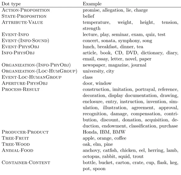
Given that the dot-type is the combination of the simple type, we can say that the dot-type of book is Info·PhysObj. In Table2.1are listed 17 dot-types.

2.2.2.3 The modes of composition

It is worth noting again here that the fundamental element in the disambigua-tion is the context. In GL three semantic transformadisambigua-tion devices are proposed that are able to capture the semantic relatedness between syntactically distinct expressions. They are:

1. Pure selection (Type matching): the type a function requires is directly satised by the argument;

(19)

Dot type Example

Action·Proposition promise, allegation, lie, charge State·Proposition belief

Attribute·Value temperature, weight, height, tension, strength

Event·Info lecture, play, seminar, exam, quiz, test Event·(Info·Sound) concert, sonata, symphony, song Event·PhysObj lunch, breakfast, dinner, tea

Info·PhysObj article, book, CD, DVD, dictionary, diary, email, essay, letter, novel, paper

Organization·(Info·PhyObj) newspaper, magazine, journal Organization·(Loc·HumGroup) university, city

Event·Loc·HumanGroup class

Aperture·PhysObj door, window

Process·Result construction, imitation, portrayal, reference, decoration, display documentation, drawing, enclosure, entry, instruction, invention, sim-ulation, illustration, agreement, approval, recognition, damage, compensation, contri-bution, discount, donation, acquisition, de-duction, endowment, classification, purchase Producer·Product Honda, IBM, BMW

Tree·Fruit apple, orange, coffee Tree·Wood oak, elm, pine

Animal·Food anchovy, catfish, chicken, eel, herring, lamb, octopus, rabbit, squid, trout

Container·Content bottle, bucket, carton, crate, cup, flask, keg, pot, spoon

Table 2.1: List of dot-types from Rumshisky, Grinberg, Pustejovsky (2007)

3. Type coercion: the type a function requires is imposed on the argument type. This is accomplished by either:

(a) Exploitation: taking a part of the arguments type;

(b) Introduction: wrapping the argument with the required type.

Type coercion, and exploitation in particular, is the very important mode here. Exploitation, as said, is the function that allows the selection of only one part of the argument, the one required by the predication.

(20)

Let’s consider the following example:

(2.13) 1. I bought the book 2. I enjoyed the book

In sentence (1) the predication of buy requires the book to be a physical object, where in the sentence (2) the verb enjoy requires the book to activate its information sense.

2.3 Computational approaches

The phenomenon of polysemy has been of interest to computational linguists too. One of the main reasons is that in several Natural Language Processing tasks, e.g. Machine Translation, the Word Sense Disambiguation is required. In the field of Computational Lexical Semantics, in regard of polysemy, the main goal to be achieved is to automatically detect the sense alternation for polysemous words. Vector Space Models (cf. Section 3.1.2) are widely used in computational semantics and in polysemy resolution too. One work worth mentioning here was done by Boleda, Pado and Utt (2012), in which they present a framework and its implementation for sense alternations prediction, by using a vector space model based on corpus data (cf. Section 2.3.1).

A totally different way to face the polysemy resolution task can be found in Rumshisky, Grinberg, Pustejovsky (2007), in which they use a clustering method based on the contextualized similarity between selector contexts (cf. Section

2.3.2).

2.3.1 VSM for alternation members

The model presented in this section, Regular polysemy: a distributional model (2012), has been developed by Gemma Boleda, Sebastian Pado, Jason Utt . They use a distributional model to detect which set of words instantiate a given type of polysemy alternation.

The goal The goal of this work, given an alternation of senses - which they call alternation - and a polysemous lemma, is to know how well that

(21)

meta-alternation can explain the two senses of the lemma. For instance, it means that given the lemma lamb, whose senses are animal, food and human, we could represent it as lambanm,lambf od and lambhum, and the meta-alternation

animal-food, they use a score function that predicts how good the meta-alternation animal-food can describe one possible combination of senses.

Their model can predict that score(animal,food,lambanm,lambf od) is greater

than score(animal,food,lambanm,lambhum), which expresses the fact that the

al-ternation animal-food can better describe the senses of lamb of animal and food.

The implementation To implement this framework they developed a Centroid Attribute Model (CAM), which is based on distributional information. In CAM there are four different elements described as vectors (cf. Section 3.2):

1. words, that are simple co-occurrence vectors;

2. lemmas, which are the centroids of all the instances of a given word; 3. meta-senses, that are the centroids of all the monosemous words with that

meta-sense;

4. meta-alternations, that are the centroids of the senses constituting the alternation.

For instance, let’s pretend we want to investigate the word lamb. We will have as many word vectors as there are occurrences of the word lamb (in a given corpus). Every word vector will be created considering the context in which the word is found. The lemma vector of lamb, on the other hand, will be only one. It will be given by the creation of a centroid of all the word vectors, which can be imagined as the sum of all word vectors.

The word vectors are also used in the creation of meta-sense vectors. For instance, in creating the meta-sense vector for the sense food, we would have to select a list of monosemous words with the sense food, such as bread, beef, vegetable, and create, again, a centroid of their word vectors so that we can have a vector representative of the distribution of words having the sense of food. The meta alternation vector is, once again, a centroid of the vectors of the words creating the alternation. For instance, the vector expressing the alternation

(22)

food-animal is created as a centroid of the vectors of food and animal. This time it will be created by the sum of two meta-sense vectors, which in this case is the one representing the sense food and the one representing the sense animal. The score-function is the result of a similarity measure (e.g. the cosine similarity, cf. Section 3.2.2.3) calculated between the lemma vector and the meta-alternation vector.

The evaluation To evaluate the model they selected a set of 40 words for each meta-alternation, among which 10 were target words expected to be selected, and 30 were distractors (by distractor they mean words sharing only one sense with the alternation or none). For instance, considering the meta-alternation food-animal, they chose 10 words with both senses food and animal, and the 30 distractors were so differentiated: 10 words having only the first sense in the alternation, which is food, and 10 having only the other sense, which is animal, and 10 words that did not have either of these two senses.

Then, the words are ranked according to the value returned by the score function calculated between the meta-alternation and each lemma. Once we have the list of words better fitting the alternation, they use the average pre-cision function to evaluate the model. This function, which is an evaluation measure from IR, evaluates how many expected words have been ranked in the top positions, with a value ranging between 1 and 0. Given that they selected 10 words as targets, they would expect those 10 words to be in the first positions. If all the targets are in the first 10 positions, the value returned by the average precision function will be 1, otherwise, if no targets are found in the top-10 positions - which means that the model has returned only distractors - the value returned will be 0. On average, the model achieves scores of 0.39, with values going from 0.709 to 0.219.

2.3.2 Contextualized similarity for alternation detection

In this section we present the model proposed by Rumshisky, Grinberg, Puste-jovsky in Detecting selectional behavior of complex types in text (2007). As pre-viously stated in Section 2.2.2, in GL the polysemous words are called complex

(23)

type (or dot object) - conversely of a simple type which are the monosemous words.

The goal The main idea of this work is to create as many clusters as many senses a polysemous word has. To do so, they use the syntactic information extracted from a corpus. Given a polysemous word, such as lunch whose dot type is food-event, they want to extract those words occurring in the same syntactic position, for instance, those words that are objects of the same verbs as the target word. Of course, dealing with polysemous words, sometimes lunch will occur with verbs found in the same context as foods (e.g. eat, cook, make) and sometimes with verbs found in the same context as events (e.g. cancel, attend, host ). Looking at the objects of verbs occurring with foods, we can expect to extract food nouns and, on the other hand, looking at the objects of verbs occurring with events, we can expect to extract event nouns. This work, relying on verbal disambiguation, is related to the issue of compositionality seen in GL (1995) (cf. Section 2.2.2).

The implementation The first thing is to select a polysemous target word -the word lunchis used in -the work. Next, -they select a specific syntactic relation, that could be the inverse direct object (which means all the verbs whose direct object is lunch), and extract all those verbs, called selector context. To formal-ize what was just described, they extract all the verbs which can be defined by the pattern (t, R, w), where t is the target word, R is the relation and w is the verb to be extracted. In this specific case in which we are considering the word lunch, we will have a pattern like (w,object,lunch), meaning that w has as object the noun lunch. This can also be written using the pattern (lunch, object−1, w), where object−1 means that lunch is object of w. After this extraction process, we can imagine obtaining a list of verbs such as: cook, serve, attend, make, eat, cancel.

Once they have extracted this set of verbs, they want to extract all the objects of those verbs that are potential contextual equivalents of the target word, because they occur in the same syntactic position as the target, with respect to the verb. This could be represented by the pattern (w, R−1, w1), where w is a verb

(24)

just extracted, R−1 is the inverse relation (if we had the inverse object relation, the inverse is the simple object relation) ans w1 is the noun to be extracted. An example could be the pattern (cook, object, w1), and an example of nouns extracted, not only with the verb cook, could be: pasta, salad, meeting, sandwich, rice, conference.

Now that they have this set of candidates for contextual equivalence, they can extract what they call the good selectors, which are those verbs having an high conditional probability with both target and candidate. It means that they want to consider only those selectors which can play an important role in disambigua-tion. For instance, the verbs eat, cook, make, etc. are very good selectors for the sense food, because they have high conditional probability with lunch and with food.

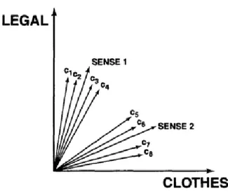
The next and final step is to create a similarity matrix (based on the con-ditional probability with the good selectors) between the contextual equivalents, and then cluster them using, as seeds, those words with the highest similarity to the target. The expectation is to have in C1 pasta, salad, sandwich, rice, etc.

and in C2 conference, festival, etc.

The evaluation The evaluation of this task has been problematic because a typical evaluation of unsupervised distributional algorithm is made by comparing the obtained results with manually constructed resources, such as WordNet, or semantically annotated corpora. However, this method of evaluation is not suit-able for this task, given that often there is a single sense for each token. The way they have found more accurate has been a manual check of the clusters. They provide the two clusters obtained by using the pattern (lunch, object−1), and it is possible to say that these clusters are very well arranged. An important thing they point out is that by looking at a partial trace of the clustering process, it is possible to see that very different words are clustered together at the beginning. Yet most of the elements in the initial clustering steps are clearly good contextual equivalents for the specific sense.

(25)

2.4 Summary

In this chapter, we examined the lexical ambiguities this work is going to focus on, that is polysemy and homonymy. We saw the differences between these two phenomenons and how they are treated in lexicography. We also saw a very important approach that could explain and solve, theoretically, the problem of logical polysemy, the Generative Lexicon. Further, we reviewed two of the most important works in polysemy resolution. The first is based on a vector space model. The second one is provided as an account for the Generative Lexicon, and it uses a different type of corpus-based approach.

A consideration that is important to mention here is that these two approaches can be used to detect the words belonging to an alternation, or the alternation proper of a given word, if these are polysemous. However, the first work cannot solve homonymy, and the authors of the second work do not seem to consider the possibility of applying the approach to homonymous words (given that in the study they provide a list of regular dot types) and do not even mention idiosyncratic complex types. In the next chapter, we are going to talk about Vector Space Model and Distributional Semantics, explaining what they are and what they can be used for.

(26)

Chapter 3 Distributional semantic models

3.1 Introduction

Distributional semantics is a field of studies in computational linguistics strongly relying on the distributional properties of words. The main theory behind distri-butional semantics is the Harris’ Distridistri-butional Hypothesis (1954), which states that words that occur in similar contexts tend to have similar meanings. Starting from this theory, computational linguists began using vectors to represent the contexts in which a word can appear. A vector is said to be representative of the meaning of a word - given that it represents its contexts. Consequently, when comparing the vectors of the word w1 and the word w2, the more contexts they

have in common, the higher the semantic similarity between these two words are. In this Chapter we are going to present the Distributional Hypothesis and the Vector Space Models (VSM), which both constitute the soul of Distributional Semantics. In the last section we will talk about a specific distributional model, called Distributional Memory (cf. Section 3.3), which has been used in this work.

3.1.1 Distributional Hypothesis

The Distributional Hypothesis constitutes the fundamentals to every distribu-tional approach to the meaning. It relies on the distributional methodology first developed in 1951 by Zellig Harris. In his Methods in Structural Linguis-tics (1951), he wrote about componential analysis in particular with regard to

(27)

phonology and morphology, and his proposal of distributional methodology was just a procedure to be followed by linguists in their analysis. What Harris sug-gests is that the very starting point should be the distribution, which can suggest some phonological and morphological properties of elements. Harris’ idea was that members of the same linguistic class behave similarly, and can therefore be grouped according to their distributional behavior. Paraphrasing his words, if we look at the two linguistic entities w1 and w2 which tend to have similar

distribu-tional properties, for example that they both occur with the same other entity w3, we may think that these two elements belong to the same linguistic class.

“The elements are thus determined relatively to each other, and on the basis of the distributional relations among them.”

What is the most surprising is that the distributional hypothesis is now known as a semantic theory even though Harris was not interested in this linguistic field. The only thought he spent on semantics in relation to the Distributional Theory can be found in a footnote, in which he argues that:

“It may be presumed that any two morphemes A and B having dif-ferent meanings, also differ somewhere in distribution: there are some environments in which one occurs and the other does not.”

More and more linguists and psychologists have tried to demonstrate the va-lidity of this theory. One of the first seminal works was made by Rubinstein and Goodenough (1965), which is also worth being remembered because it is one of the very first studies which explicitly formulated and investigated the distribu-tional hypothesis. In their work they asked 51 undergraduate students to provide synonymy judgments on 65 pairs of words, which were later compared with dis-tributional similarities. As expected, their experiment demonstrated first that “words which are similar in meaning occur in similar contexts.”(Rubinstein and Goodenough, 1965). Afterwards, almost 30 years later, a very similar experiment was done by Miller and Charles (1991). The principal difference between these two experiments was the number of pairs (30 instead of the original 65) and the number of subjects judging the synonyms (38 instead of 51). Even with these differences, the experiment led to a similar result. The Distributional Hypothesis can be stated as follows (Lenci 2008):

(28)

The degree of semantic similarity between two linguistic expressions A and B is a function of the similarity of the linguistic contexts in which A and B can appear.

This theory is the centerpiece of distributional semantics along with Vector Space Models. In the next section we are going to explain the relation between this theory and the mathematical structures that make its implementation pos-sible.

3.1.2 Vector Space Models

Vector Space Models, henceforth VSM, are those approaches to meaning which describe documents or words in terms of their distributional properties. As the name suggests, they use a mathematical structure called vector, which is very versatile, insomuch as it is used both in artificial intelligence and cognitive science. The first example of using VSM in Artificial Intelligence can be illustrated by SMART project (Salton, 1971), which was developed by Salton for an information retrieval system. The idea behind this system seems to be very intuitive: if a document can be represented as a point in a space (a vector in a vector space), points that are close together in this space are semantically similar, and points that are far apart are semantically dissimilar.

Since then, VSM-based related models have been developed, such as Latent Se-mantic Analysis (LSA) (Deerwester et al., 1990; Landauer and Dumais, 1997) and Hyperspace Analogue to Language (HAL) (Lund, Burgess, and Atcheley, 1995; Lund and Burgess, 1996).

The idea behind the VSMs is that any item can be described by a list of features. A feature can be the salience of an attribute for a concept, or in infor-mation retrieval it can be the frequency of a term in a document, or in distribu-tional semantics it can be the probability for a word to have an element in its environment.

(29)

3.2 Distributional Semantic Models

In this work our focus will be on Distributional Semantic Models, DSMs. To give a brief explanation of what a DSM is, we could say that it is the most natural implementation of Harris’ statement that words with similar meaning tend to occur in similar contexts (cf. Section 3.1.1).

It is obvious that the key role here is played by the words surrounding a target word, and the two elements needed in getting this kind of information are a solid language representation and some statistical methods. Corpora are the easiest way to get a language representation. They are very important in distributional semantics because we need a textual source of information that can be used to automatically extract the words distributional properties. Statistics, on the other hand, is fundamental because it is used to determine the most salient contextual features based on the association strength between a word and a certain context.

Let’s pretend that our corpus is the following sentence and that we want to extract the distributional properties of each word in it.

(3.1) When the time will come, I will arrive in time.

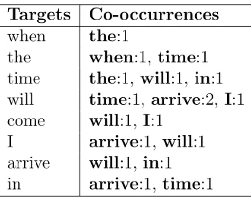
When collecting distributional information the first thing to think of is: what is the context? The problem is that there are many types of contexts. The context might be the whole sentence in which the word appears, it might be the words surrounding the target, or it might be the words syntactically connected to the target. In this example, we will let the context be the words surrounding the target, which means the preceding and succeeding word. In such a situation, the context of the word “the” will be when and time, the context of the word “in” will be arrive and time. A better way to show the contextual information we can collect from this sentence would be to create a co-occurrence table using the row counts of the co-occurrences.

To create a co-occurrences table we use word types instead of tokens. This is necessary because in the table we do not want a list of all the words and the relative context in which they appeared, but we want the representation of the generalization of a word and all the contexts in which it has been found.

The goal, in this step, is to create vectors representing the word context, and this table can easily be translated in a word-context matrix (Table 3.2).

(30)

Targets Co-occurrences when the:1

the when:1, time:1 time the:1, will:1, in:1 will time:1, arrive:2, I:1 come will:1, I:1

I arrive:1, will:1 arrive will:1, in:1 in arrive:1, time:1

Table 3.1: Table in which are presentend the co-occurrences with the Targets and their frequency.

Words

when the time will come I arrive in when 0 1 0 0 0 0 0 0 the 1 0 1 0 0 0 0 0 time 0 1 0 1 0 0 0 0 will 0 0 1 0 0 1 2 0 come 0 0 0 1 0 1 0 0 I 0 0 0 0 1 0 1 0 arrive 0 0 0 1 0 0 0 1 in 0 0 1 0 0 0 1 0

Table 3.2: Co-occurrence matrix

In this matrix each row is a vector representing a word, and the columns represent each time in which the word appears.

Having this structure in mind, it is worth mentioning the formalization of the Distributiona Semantic Model given by Lowe (2001) and Pado and Lapata (2007). They define a DSM as a quadruple 〈B, A, S, V 〉where B is the set of elements to be defined, A is the set of contexts used to define the elements in B, S is a similarity measure used to compute the similarity between the elements in B, and V is an optional transformation which reduces the number of elements in A. In this table we can clearly see that we have B, that is made by the words in the sentence, and A, that is also made by the words in the sentence, but here they

(31)

are considered contexts. These two, B and A are the fundamental parts in the definition of a DSM. Additionally, we still need a similarity measure and, maybe, a transformation which can reduce the matrix dimensionality. In the following sections we will focus on words and contexts, looking at the association measures used to weigh the correlation between a term and a context (cf. Section 3.2.1) on the most used similarity measures (cf. Section 3.2.2) and on some techniques of dimensionality reduction (cf. Section 3.2.3).

3.2.1 Language and statistics

In Table 2.3 we represented a co-occurrence matrix. In this section we are going to present what is needed to create a DSM.

3.2.1.1 The words

The first thing in creating a DSM is to select the words we are interested in and eliminate those words not semantically relevant, such as articles, conjunctions, prepositions, adverbs, etc., which are all the words we do not need to have rep-resented as targets. Therefore, they are grouped together in a set of words called a stop list. We do not need these words as context either, because they are not significant in determining the meaning of the words since they can easily occur with a huge number of words. For example, in the sentence in Sentence 3.2, the only relevant word we should represent in a semantic space would be time, come and arrive, because all the other items are just adverbs, articles, prepositions and pronouns that are included in the stop-list. After this very important step there is one left to be performed, which is normalization. Every time we build a DSM we have to consider the word lemmas and not the inflected forms.

3.2.1.2 The contexts

The most important thing is to define what a context is in regard of our task. In Table 3.2 we have the simplest example possible for context matrix, because the context is represented by the simple words in the sentence, and when a target word had a context word preceding or following it, it was considered to be belonging

(32)

to that context. Sometimes the span of the co-occurrence window4 is set to be bigger than 1, and it is possible that we would select words syntactically related to other items in the sentence when using a bigger span. For instance, let’s consider the sentence “while you eat your sandwich I watch the television”. If we want to represent the distribution of the word sandwich, even considering the words in a window large 2, we would have the contexts eat and watch, where the second context is not representative at all of the distribution of sandwich.

This problem can be solved considering a different kind of context, the syn-tactic context. The only difference with the one we have presented above is that, only words surrounding the target that are syntactically related to it are considered. In this way, we would automatically not consider the verb watch as a context of sandwich because there is no relation between these two lexical items, even though they occur very close in the sentence. Using such a context, we can imagine a DMS in which there are the represented words sandwich, cake, dog and cat and where, as already said, the contexts are exclusively the lexical items that, in a given span, have a syntactic relation with those words, supposedly verbs and adjectives.

Words

feed prepare eat cute bark yummy jump make pizza 0 143 86 0 0 24 0 128

cake 0 25 12 0 0 30 0 102 dog 98 0 29 18 9 0 38 0

cat 46 0 32 24 0 0 59 0

Table 3.3: Co-occurrence frequency matrix with syntactic relations

In the Table 2.4 it is very interesting to note that the verb eat is a context for all the words we have in the DSM, because it is both true that “someone is eating a sandwich” and that “a cat is eating a mouse” and therefore that eat can occur with both words, even though it occurs with the targets in a different syntactic relation.

In Section 2.3.2 we presented a work by Rumshisky, Grimberg, Pustejovsky

4 _{A occurrence window is an unstructured span of tokens surrounding a word. A}

co-occurrence window with span 5 means that we want to consider 5 words after and 5 words before the target word.

(33)

that used a sort of syntactic context, because for each target - in that case we have presented the word lunch - they selected a set of verbs for whom lunch was a direct object - for instance cook, serve, attend. In that case a DSM was not used, but if we created one with this kind of structure we would imagine a DSM in which in the rows would be those words we need to have a semantic representation for and the columns would be the verbs those words can occur with, specifying which relation the verbs must have with the words.

Considering the matrix we have shown in Table 3.3, the verb eat would be split into two different contexts, eat-subj and eat-obj, where dog and cat would be found in the context of eat-subj, because they are the subjects of that verb, and sandwich and cake would count as occurrences of the context eat-obj, because they are the objects of the verb.

Baroni and Lenci (2010), as we will see in more detail in Section3.3presented a DSM, Distributional Memory, with these three dimensions we are talking about, the target words, the contexts, and the syntactic relations. Looking back to the quadruple defining a DSM, we could say that for each word B we have a set of contexts A, where A is given by the combination of a context word C and a syntactic relation D. According to this, we could rewrite the quadruple as a quintuple with 〈B, C, D, S, V 〉.

3.2.1.3 The dimensions

So far, every matrix we presented had the raw counts of occurrences as its di-mensions. In Table 3.3, the word sandwich has a value of 143 with the context prepare, where 143 is the number of times these two words have occurred together. This value is not so interesting, because it can tell us the frequency of an event, but can not make explicit whether or not that event has some relevance. Let’s consider the verb make. In Table 2.4 we see that both sandwich and cake have a high frequency with the context make, but we do know that make is not a relevant context for these words. By relevant context we mean that it is frequently used exclusively with a particular semantic set of words: for instance, the verb bark is a relevant context for the word dog because we expect to see it in contexts with dogs and nothing else. In information theory, for instance, a surprising event is

(34)

considered as having more information content than an expected event (Shan-non, 1948). To evaluate how peculiar a context is for a given word, the most used association measure is the Pointwise Mutual Information (PMI), (Church and Hanks, 1990; Turney, 2001).

PMI(w, c) = log p(w, c) p(w) · p(c) (3.1)

Given the word and context, the PMI compares the joint probability of the word and context with the probability of these two items occurring independently from each other.

Let’s consider again Table3.3 and let’s try to write, instead of the frequencies, the PMI values. To calculate the probability of these items we need to know the number of events this matrix f(m) is recording, and we do it as defined in the following formula. f (m) = nw X w=1 nc X c=1 fwc p(w, c) = fwc f (m) p(w) = Pnc c=1fwc f (m) p(w) = Pnc c=1fwc f (m) p(c) = Pnw w=1fwc f (m) (3.2)

Even though the matrix in Table 2.4 is not representative of all the contexts in which those words can appear and, therefore, is not representative of all the

(35)

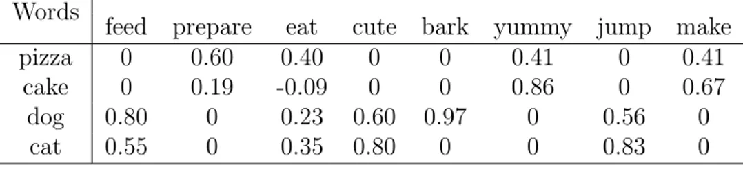
semantic features those words can be represented with, we are trying to translate this frequency matrix in a PMI-matrix following the definitions we have presented above. By doing so, we would have a matrix that looks like the following one.

Words

feed prepare eat cute bark yummy jump make pizza 0 0.60 0.40 0 0 0.41 0 0.41

cake 0 0.19 -0.09 0 0 0.86 0 0.67 dog 0.80 0 0.23 0.60 0.97 0 0.56 0

cat 0.55 0 0.35 0.80 0 0 0.83 0

Table 3.4: Co-occurrence matrix with PMI values

In Table3.4there are some things worth noting. The first thing is the behavior of the context eat. As already mentioned, it is a very common context, insomuch as every word in the matrix appear in it. Given this peculiarity, we can see that the PMI does not have a high value in either of the words. The second important thing concerns the context bark. Contrary to the context eat, which is shared by all the words in the matrix, bark is an effectual context only for the word dog, which is the reason why it has a PMI of 0.97 even if the raw frequency of it was only 9.

A variation of PMI is the Positive Pointwise Mutual Information, in which all PMI negative values are replaced with zero. For instance, the value in Table 3.4 for (eat, cake) would be replaced by 0, given that the PMI returned a value lower than 0.

However, the PMI, as well as the PPMI, are biased towards infrequent events. If two words a and b occur in the corpus only once, and they occur together, the PMI would return a very high value, given that these two words have maximum association. A variation of PMI that can solve this problem is the Local Mutual Information (LMI), which also considers the frequency of the event.

LMI(w, c) = f (w, c) ∗ log p(w, c) p(w) · p(c) (3.3)

(36)

By doing so, simply multiplying the PMI with the frequency of the pair, we have an expected high value only for those pair of words frequently occurring together. Of course, the value returned by the LMI is no longer a ranged value because of the frequency multiplication.

3.2.2 Similarity measures

Starting from the DH statement “words with similar meanings tend to occur in similar contexts”, to achieve our goal of computing the semantic similarity between words, we have to look at the contexts in which the words appear. Before discussing similarity measures in detail, it is necessary to point out what we refer to when we talk about similarity. The computation of similarity using DSMs is actually what is called attributional similarity in cognitive science, because sim(a,b) depends on the degree of correspondence between the attributes - in this case contexts - of the words a and b. In this work we use the word similarity to indicate semantic relatedness.

There are different ways to compute the similarity between vectors. We will present three different classes of similarity measures. The first kind relies on the number of contexts shared by the word vectors compared: these are the Jaccard and Dice coefficients. The second kind focus on the geometrical properties of vectors as points in a high-order distributional space, with the aim of computing the distances between them: these are the Euclidean and Manhattan distances. The third way to compute the similarity, which is the most complex as well as the most used, is the Cosine similarity, which relies on the geometrical properties of the vectors as a line segment which originate in the origin and ends at the point defined by the vector.

3.2.2.1 Jaccard and Dice Coefficients

These two measures are often used in statistics to compute the similarity between items. The idea of both these coefficients is to measure the overlap between the dimensions of two vectors A and B.

(37)

J(A, B) = |A ∩ B| |A ∪ B| (3.4)

It computes the number of elements the item A has in common with the item B, over the number of the unique elements as result of the union of A with B . Let’s consider the items in Table 3.4, where A is the word dog and B is the word cat. The J(dog,cat) is 0.80, because the size of the elements they share is 4, and the size of the union of the elements is 5 (bark appears to be a context only for dog).

The Dice coefficient works in a very similar way. It is defined as follows:

D(A, B) = 2|A ∩ B| |A| + |B| (3.5)

The Dice coefficient computes two times the number of elements in common between A and B, over the number of elements in A and B. If we would compute D(dog,cat) the value would be 0.88, because two times the common elements is 8, over the length of dog, which has 5 elements, summed to the length of cat, which is 4: that is 8 over 9.

Both these similarity measures range between 0, when there are no elements in common and 1, when comparing two identical items.

3.2.2.2 Euclidean and Manhattan Distances

As already said, the Euclidean and Manhattan distances rely on the geometrical properties of vectors. These are measures commonly used in geometry.

The Euclidean distance is what is commonly called “ordinary” distance, be-cause in a bi-dimensional space it would be the simple distance between two points, which is what is computed with the Pythagorean formula. It is possible

(38)

to calculate the Pythagorean formula when dealing with vectors, even if it is a little more complicated. The idea is to compute the linear distance between the points defined by the vectors.

The Euclidean distance is defined as follows:

E(A, B) = v u u t n X i=1 (Ai− Bi)2 (3.6)

Applying this formula again to the words dog and cat we would have E(dog,cat) being √0.252 _{+ 0.12}2_{+ 0.20}2_{+ 0.97}2_{+ 0.27}2_{, which yields 1.06. Different from}

the Jaccard and Dice coefficients, the obtained value with this distance measure is not ranged. It is just a number representing the distance between two points, which, of course, is inversely proportional with the similarity of the compared words.

However, every measure of distance can be easily converted to a measure of similarity by inversion or subtraction. This means that:

sim(A, B) = 1 dist(A, B)

sim(A, B) = 1 − dist(A, B) (3.7)

The Manhattan distance works in a similar way. The main difference concerns the way that the distance between the points defined by the vector is computed. In the Euclidean distance a linear distance is computed, where in the Manhattan distance it is necessary to take the sum of the lengths of the projections of the line segment between the points onto the coordinate axes.

(39)

M(A, B) = n X i=1 |Ai− Bi| (3.8)

As it is possible to see, the main difference in the formula with the Euclidean distance is the absence of the square root and the raise to power of two. Using this formula to compute the similarity - or the distance - between the words dog and cat we would have 0.25 + 0.12 + 0.20 + 0.97 + 0.27, which yields 1.81. As in the Euclidean distance, the resulting value is directly proportional with the distance, but it can be converted to a measure of closeness/similarity as well.

3.2.2.3 Cosine similarity measure

The most popular way to measure the similarity between two vectors is to com-pute their cosine. We know that a vector can be represented as a line segment which originates from the origin in a Cartesian plane and ends in the point de-fined by the vector itself. When we want to calculate the similarity between two vectors we want to get the cosine of the angle they create. From trigonometry we know that the cosine of the angle ϑ created by a line which originates in the origin of the plane is the projection of the radius on the x axis. With the cosine similarity we want to know the cosine of the angle created by the vectors we want to compare.

The cosine similarity is defined as follows:

cos(A, B) = − → A ·−→B |−→A ||−→B | (3.9)

As it is possible to see in the formula above, the cosine similarity is the dot product of two vectors normalized to unit length. The dot product can be formalized as follows:

(40)

− → A ·−→B = n X i=1 AiBi (3.10)

It means that the corresponding dimensions of the two vectors A and B have to be multiplied and then summed up.

The normalization is needed because the idea behind this similarity measure is that the vector lengths are not an important element for the computation. In fact, the computation of cos(ϑ) is strictly dependent on the width of the angle, and not on the length of the vectors creating it. To set the vectors length to 1, the normalization can be defined as:

|−→A | = v u u t n X i=1 − → A2_i (3.11)

Let’s try to compute the cos(dog,cat). First of all, we have to compute the dot product between the vectors of the words dog and cat. The first steps in the computation are 0.80 · 0.55 + 0.23 · 0.35 . . . 0.48 · 0.4648, which is equal to 1.4653. The second step is to normalize the vectors, following the formula we presented above. We have to compute the normalization for both vectors and then multiply the resulting values. The value normalizing the dog vector is 1.519, and the value normalizing the cat vector is 1.324. The last step is to compute the ratio 1.4653/2.01161, which gives us that cos(dog,cat) = 0.72.

As in the Jaccard and Dice coefficients, the cosine returns a ranged value, but it ranges between 1 when the vectors are identical and 0 when they are orthogonal.

3.2.3 Dimensionality reduction

The last thing we have to talk about, concerns some techniques of dimensionality reduction. Table 3.3 presents a very small matrix composed by 4 items, each one of which uses 8 different dimensions to be described. However, in real tasks

(41)

it is common to deal with huge matrices with million of dimensions, which are populated primarily with zeros. In those cases, computing the similarity becomes a computationally intensive task. Recalling the last element of the quadruple〈B, A, S, V〉, we will talk about the V, which is the component represented by the optional transformation which operates a reduction of the matrix. We will present the two most used techniques of dimensionality reduction, which are the Singular Value Decomposition (SVD) and the Random Indexing (RI). These two techniques operate in completely different ways. For example, where the SVD operates a smoothing on an already built matrix, the RI is a technique to create a matrix operating a reduction from the beginning.

3.2.3.1 Singular Value Decomposition

The Singular Value Decomposition is a linear algebra technique which operates a factorization of a complex matrix. The main idea behind it is that any matrix can be decomposed into the product of three matrices with each representing a particular aspect of it. The formalization of the SVD is:

M = U ΣV

(3.12)

This formula shows how the decomposition is operated upon the matrix M. Let’s suppose M is mxn matrix. U and V would be orthogonal matrices re-spectively with mxm and nxn. Σ would be a matrix with the original matrix proportions mxn but with the singular values of the matrix M in its diagonal and zero values in all the other dimensions. In a matrix M with m=3 and n=4 UΣV would be: U = · · · · · · · · · Σ = · · · · · · · · · · · · V = · · · · · · · · · · · · · · · ·

(42)

Having the matrix decomposed like this, it is possible to operate a smoothing, which implies the reduction of noise as well as sparsity. This technique is called Truncated SVD (Deerwester et al., 1990).

The most interesting component of M in operating the TSVD is the Σ matrix. It is a diagonal matrix, which we can be imagined as follows:

Σ = σ1 0 0 0 0 0 σ2 0 0 0 0 0 σ3 0 0 0 0 0 σ4 0 0 0 0 0 σ5

The most interesting property of the Σ matrix is that σ1 ≥ σ2 ≥ σ3 ≥ σ4 ≥

σ5 ≥ 0. When we set the k value, which is the size we expect our truncated

matrix to have, we are actually choosing to set all but the first k largest singular values equal to zero and to use only the first k columns of U and V. Then, the last step the TSVD performs is the composition of the matrix based on the new components.

3.2.3.2 Random Indexing

Random Indexing (RI) (Sahlgren, 2005) is another technique which operates an approximation of a matrix, based on Kanerva’s work on sparse distributed rep-resentations (Kanerva 1988, Kanerva et al., 200, Kanerva et al., 2001). Different from what happens with the SVD, which needs to have an already computed matrix to operate the reduction, RI creates a reduced matrix from the beginning. In Section 2.2 we saw that the first step to create a matrix is the computation of a co-occurrence matrix and then the extraction of context vectors from it. RI directly creates the vectors by looking at the contexts in which the words appear.

The algorithm of random indexing can be summarized in two steps:

1. For each word in the data is assigned a randomly generated representation with dimensionality δ, where δ is a fixed constant. This vector, known as index vector, has very few non-zero elements, which can be only +1s or -1s, in equal number.

2. To create the distributional space, the vector of each target word is com-puted by summing the index vectors previously - randomly - generated.

(43)

One of the most interesting aspects of Random Indexing is the possibility of dealing with a huge amount of data, which would be impossible if computing a matrix and then operating SVD. Even if it seems that this technique would return vectors different from the ones computed in the traditional way - which means computing first the co-occurence matrix - it has been validated in several experiments that shows it performs as well as other DSMs.

3.3 Distributional Memory

In this chapter we have presented the Distributional Semantic Models and how they work. In the following section we will present one particular DSM, Distri-butional Memory (Lenci, Baroni, 2010), which is a general framework for distri-butional semantics. It was developed based on the idea that it is unnecessary to build a new DSM for every semantic task. First, because there is an high risk to create a model overfitting the task, and second because, from a purely cognitive perspective, this is not the way the human’s semantic memory works.

3.3.1 The framework

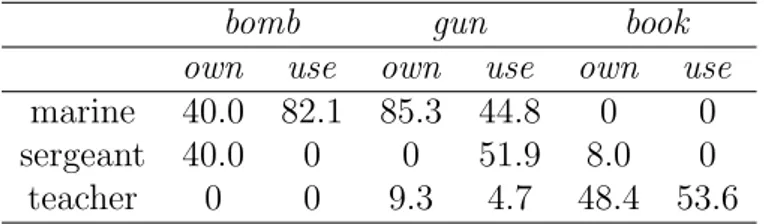
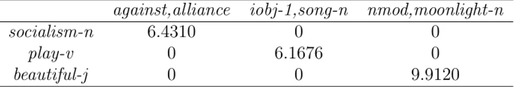
The goal of DM is to provide a structured DSM, where structured means that co-occurrence statistics have been collected along with the syntactic informa-tion. DM is presented as a set of weighted tuples, which can be represented as 〈w1,l,w2〉. This tuple expresses that w1 is linked to w2 through the relation l. An

example could be the tuple〈marine,use,bomb〉 which represents the distributional information of marine occurring in the same context as bomb, where use is the syntagmatic relation occurring between these two words. It is worth specifing that every tuple in DM is also represented with the inverse relation, which means that for the tuple 〈marine,use,bomb〉, the tuple 〈bomb,use−1,marine〉 also exists. As we said, every tuple is then weighted by counting the occurrences of the tuple and weighting the raw counts by local mutual information (cf. Section

3.2.1.3).

What we have is a structure like the following one:

Regular polysemy: A distributional semantic approach