Human Long Bones in vitro biomechanical characterization

(1)

Alma Mater Studiorum – Università di

Bologna

DOTTORATO DI RICERCA

IN BIOINGEGNERIA

Ciclo XXI

Settore scientifico disciplinare di afferenza: ING-IND/34

TITOLO TESI

CARATTERIZZAZIONE BIOMECCANICA IN VITRO

DELLE OSSA LUNGHE DELLO SCHELETRO UMANO

HUMAN LONG BONES IN VITRO

BIOMECHANICAL CHARACTERIZATION

Presentata da: Ing. MATEUSZ JUSZCZYK

Coordinatore Dottorato:

Relatore:

Prof. Angelo Cappello

Prof. Luca Cristofolini

(2)

Sommario

La presente tesi descrive i risultati delle ricerche svolte durante il Dottorato. in Bioingegneria. L'obiettivo di questa ricerca era quello di valutare le proprietà biomeccaniche di sei ossa lunghe umane (radio, ulna, omero, femore, tibia e perone), come contributo alla creazione del "Living Human Digital Library" (LHDL). La ricerca presentata in questa tesi è stata effettuata presso il Laboratorio di Tecnologia Medica (LTM) dell’Istituto Ortopedico Rizzoli (Bologna), partner all’interno del progetto LHDL.

Un osso lungo è il principale argomento di tutti gli studi presentati in questa tesi. Ogni osso può essere considerato come tessuto, struttura e organo simultaneamente, tuttavia verranno qui presentati solo gli aspetti studiati a livello di organo. Le ossa lunghe sono state ampiamente studiate in passato e la loro biomeccanica è nota, ma finora non sono state presentate descrizioni inter-disciplinari e multi-livello dell’apparato muscolo-scheletrico umano. In realtà, il progetto LHDL mira ad indagare due cadaveri umani, partendo dal livello globale del corpo attraverso il livello organico fino quello proteico, creando un dataset multi-livello specifico dei soggetti analizzati. All'interno di questo quadro, l'obiettivo di questa tesi è stato quello di misurare, per ciascuno dei sei segmenti ossei la rigidità, la resistenza e la distribuzione delle deformazioni

Lo sviluppo di metodologie in grado di garantire elevata qualità dei dati e futura compatibilità spaziale per la fusione tra livelli strutturali è risultata essenziale all'interno di questo studio.

Pertanto, un sistema di marcatori per le diverse tecniche di imaging medico è stato sviluppato con lo scopo di aiutare la fusione tra diverse misure a livello di corpo, organi e segmenti. Utilizzando i marcatori sviluppati è stato possibile combinare dati provenienti da TAC, RMN e cinematica passiva e, inoltre, preservare le i segmenti ossei da qualsiasi rischio di danni meccanici, come ad esempio l'esecuzione di fori previsti dalla tecnica utilizzata in precedenza.

Una definizione univoca dei sistemi di riferimento della biomeccanica muscolo scheletrica è stata estremamente importante. Soprattutto in virtù del fatto che dovevano essere svolte misure multi-livello. Pertanto tre sistemi di coordinate anatomiche sono

(6)

stati confrontati per definire quello maggiormente riproducibile per il tracciamento dei piani anatomici.

Parte degli obiettivi del laboratorio sono stati la creazione e validazione di modelli ad elementi finiti (FEM) disegnati sul soggetto. Pertanto, è stato necessario fornire alcuni dati per la definizione delle condizioni al contorno, di fondamentale importanza per una accurata validazione di modelli FEM.

Prima di tutto, allo scopo di riprodurre la posizione delle forze risultanti del giunto, durante il test in vitro delle ossa lunghe, è stata sviluppata una apposita cella di carico. Successivamente, per misurare il punto iniziale di frattura, necessario per la validazione dei modelli FEM per la predizione di fratture ossee, una nuova tecnica chiamata Crack Grid è stata sviluppato.

La Crack Grid ha consentito di distinguere il punto di frattura con una risoluzione spaziale di 3 mm, fornendo dati sufficientemente precisi per la convalida dei modelli FEM e fornendo ulteriori informazioni relative alla meccanica delle strutture ossee. Tuttavia questa tecnica non è limitata solo alla convalida dei modelli FEM, ad esempio può essere applicata per verificare le relazioni tra la frattura e l’orientamento del collagene nella stessa regione. Inoltre, la Crack Grid può essere applicata in altri ambiti della scienza dei materiali, come i materiali compositi, le ceramiche, ecc, dove il punto di innesco e propagazione della frattura sono temi di studio comuni. I risultati di questo studio possono essere distinti come: legati allo sviluppo dell’enciclopedica digitale prevista all’interno del progetto LHDL; ma anche risposte a specifici quesiti di ricerca.

I dati relativi alle richieste del progetto LHDL sono la distribuzione delle deformazioni di segmenti ossei interi, la rigidezza e la resistenza per uno scenario definito a priori (torsione, flessione a quattro punti), dipendente dal tipo di segmento osseo.

Le relazioni di velocità e direzione di carico sono state valutate attraverso lo studio del comportamento viscoelastico e non lineare della struttura ossea.

All’interno di questa tesi sono stati condotti due studi specifici riguardanti il femore prossimale. Il primo la distribuzione delle deformazioni del femore prossimale. Si è trattato di un dettagliato studio, basato sull’utilizzo di strain-gauge, mirato alla comprensione delle capacità di carico della struttura ossea.

(7)

- 6 -

Il secondo studio riguarda le fratture spontanee del femore prossimale. Non esistono evidenze, ne consenso scientifico, relativamente i più rilevanti scenari di carico. Lo scopo di questo lavoro è stato quello di sviluppare e validare un metodo sperimentale per replicare in vitro scenari di fratture spontanee, basandosi su carichi clinicamente rilevanti.

Una combinazione di tecniche computazionali e sperimentali è stata applicata per replicare le fratture del femore prossimale con grande ripetibilità e riproducibilità. Per prima cosa è stato identificato lo scenario di carico più rilevante tramite l’utilizzo di un modello numerico. È stato poi evidenziato che non è necessario includere la funzione dei muscoli quando è in analisi la frattura del collo del femore. Il set-up sperimentale è stato poi progettato di conseguenza. Modelli di frattura clinicamente rilevanti sono stati ottenuti. Il metodo proposto può essere usato per investigare le ragioni ed i meccanismi di fallimento di femori prossimali sani ed operati.

Il lavoro svolto sino ad ora ha anche alcune applicazioni pratiche. Infatti la conoscenza pratica sviluppata testando i femori prossimali è stata applicata anche all’ottimizzazione di protesi prossimali di femore.

(8)

SUMMARY

The present thesis describes results of the research performed throughout the Ph.D. in Bioengineering. The aim of this research was to evaluate biomechanical properties of the six human long bones (radius, ulna, humerus, femur, tibia and fibula), as a contribution in the creation of the “Living Human Digital Library”(LHDL). The research presented in this thesis was carried out at the Laboratorio di Tecnologia Medica (LTM) of Istituto Ortopedico Rizzoli (Bologna), a partner to the LHDL-project.

A long bone is the main subject for all studies presented within this thesis. Each bone can be considered as a tissue, a structure and an organ simultaneously, however just the organ level is considered here. Long bones have been widely studied in the past and their biomechanics is well known, but so far there is no multi-level, inter-disciplinary description of the human musculo-skeletal apparatus. In fact, the LHDL project aimed to investigate two human cadavers from whole body level through organ level up to protein level giving a subject specific multi-level dataset. Within this framework, the goal of this thesis was to measure for each of the six bone segments whole bone stiffness, strength and strain distribution.

The development of methodologies able to ensure both high data quality and future spatial compatibly for data merging between structural levels was essential within this study.

Therefore, marker for different medical imaging techniques was developed to assist merging of different measurements of the whole body, body-segments and organs. Using the developed markers it was possible to support CT, MRI and joint passive kinematics measurements and moreover to preserve long bone segments from any mechanical damage, such as caused by drilling holes, contrary to a previously used marker technique.

A univocal definition of coordinates systems was extremely important in musculoskeletal biomechanics especially given that multi-level measurements had to be conducted. Therefore three anatomical coordinate systems were compared to define of the most reproducible coordinate system for tracing of anatomical plans.

Part of the LTM goals was the creation of subject-specific finite-element models (FEM) and to validate them. Therefore, it was necessary to provide some data to define the boundary conditions, crucial for accurate validation of the FEM. First of all, to reproduce the position of the resultant joint force during in vitro tests of long bones, a

(9)

- 8 -

load cell has been developed. Thereafter, to measure the crack initiation point, which was needed to advance FEM predicting bone fracture, a novel technique called the Crack Grid was developed.

The Crack Grid permitted to distinguish crack initiation point with 3mm spatial resolution, providing accurate data for the FEM validation and delivering extra information related to bone structure mechanics. However this technique is not limited only to the FEM validation, e.g. can be applied to verify relations between the fracture and collagen orientation in this same region. Moreover, the crack grid can be applied in the other materials science like composites, ceramics etc, where crack initiation point and fracture propagation are common subjects of study.

Results of this study can be distinguished as related to: LHDL, encyclopaedic like dataset and; specific research questions.

The data related to LHDL project demands are whole bone strain distribution, stiffness and strength for a prior chosen loading scenario, depending on the bone segment (torsion, four point bending). A loading direction and loading velocity relations were assessed providing deeper insight into bone structure non linearity and viscoelastic behaviour.

Within this thesis two specific studies addressing the proximal femur were conducted. The first one deals with strain distribution in proximal femur. It was a detailed strain-gauge based study aimed at giving an insight to understanding of proximal femur structure and its load bearing capabilities. The second one is approaching spontaneous fractures of proximal femur. There is no evidence, nor consensus on the most relevant loading scenario. The aim of this work was to develop and validate an experimental method to replicate spontaneous fractures in vitro based on clinically relevant loading. Combinations of experimental and computational techniques were applied to replicate fractures of the proximal femur with a high repeatability and reproducibility. First a numerical model indicated the most relevant loading scenario. Furthermore, it was found that it is not essential to include the muscles when investigating head–neck fractures and consequently the experimental setup was designed. Clinically relevant fracture modes were obtained. The proposed method can be used to investigate the reason and mechanism of failure of natural and operated proximal femurs.

The work done so far had also some practical application. In fact the know-how developed during testing the proximal femur was applied to testing and optimizing proximal epiphyseal replacement of the femur.

(10)

(11)

- 10 -

(12)

1.1 Bone- an engineering approach

Bone can be considered as a tissue, an organ, a structure in this same time. However, the most relevant to the aims of this thesis are mechanical behaviours of cortical and trabecular bone.

Bone is an inhomogeneous material because it consists of various cells, organic and inorganic substances with different material properties. In mechanical terms bone is a composite material with various solid and fluid phases. The inorganic component of bone makes it hard and relatively rigid, and its organic component provides flexibility and resilience. The composition of bone varies with age, sex, type of bone, type of bone tissue and presence of bone disease.

Bone is an anisotropic material because its mechanical properties in different directions are different. That is, the mechanical response of bone is dependent upon the direction as well as the magnitude of the applied load. For example, compressive strength of bone is greater than its tensile stress. Moreover bone possesses viscoelastic (time dependent) material properties; hence the mechanical response of bone is dependent on the rate at which the loads are applied. Bone can resists rapidly applied loads much better than slowly applied loads: bone is stiffer and stronger at higher strain rates.

1.1.1 Cortical Bone

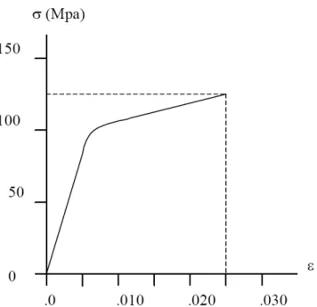
Mechanical properties of cortical bone have been well documented. Traditional mechanical testing techniques such as uniaxial tensile or compressive testing and three-points or four-three-points bending have been used for measuring these properties [1] as well as ultrasonic techniques, by subjecting the bone to ultrasound and measuring the velocity of the sound [2]. A typical tensile stress-strain diagram for the cortical bone is shown in figure 1.

(13)

- 12 -

Figure 1 Tensile stress-strain diagram for human cortical bone loaded in the longitudinal direction (strain rate ε’=0.05 s-1)

This σ-ε curve was drawn using the averages of the elastic modulus, strain hardening modulus, ultimate strain and ultimate stress values determined for the human femoral cortical bone by Really et al.[1]. Reilly at al tested specimen of bone tissues (human and bovine) under tensile and compressive loads applied in the longitudinal direction at a moderate strain rate (ε’=0.05 s-1). The diagram that can be considered representative of the behaviour of cortical bone under tension or compression shows three distinct regions. In the initial region the behaviour is linear-elastic and the slope of the straight line is equal to the elastic or Young modulus E of the bone, which in the example is almost 17 GPa. In the intermediate region the bone exhibits a non-linear elasto-plastic behaviour. Material yielding also occurs in this region. In the final region, the bone exhibits a linearly plastic material behaviour and the σ-ε diagram is another straight line. The slope of this line represents the strain hardening modulus of bone tissue, which was about 0.9 GPa in the example.

The elastic modulus and the strength value are dependent on the rate at which the loads are applied[3]. This viscoelastic nature of bone can be described with the qualitative diagram plotted in Figure 2.

(14)

Figure 2 The strain rate dependent stress-strain curve for cortical bone tissue

The specimen of bone tissue subjected to a rapid loading generally shows an increase in bone fragility and a parallel increase in the elastic modulus. With respect to a specimen loaded more slowly, there is a reduction in the post-elastic phase (it can even lack) and in the strain to failure as well as an increase in the ultimate stress. The absorbed energy, which is proportional to the area under the σ-ε curve, by the bone tissue generally decreases with the strain rate.

Bone will bear a higher stress if it is loaded at a higher strain rate. Carter and Caler [4] found an empirical relationship between failure stress and strain, or stress, rate:

The stress-strain behaviour of bone is also dependent upon the orientation of bone with respect to the loading direction. This anisotropic material behaviour can be qualitatively described by the diagram plotted in Figure3.

(15)

- 14 -

Figure 3 The direction dependent stress-strain curve for bone tissue.

The cortical bone shows a larger ultimate strength and a larger elastic modulus in the longitudinal direction than in the transverse direction. Moreover, bone specimens loaded in the transverse direction fail in a more brittle manner, without showing a considerable yielding, as compared to bone specimens loaded in the longitudinal direction.

Although the qualitative behaviour of cortical bone described previously is commonly accepted, still a great range for the values of the mechanical characteristics can be found in literature for many reasons. First of all, differences in the measured values can be due to the different treatment of specimens. It has been shown that drying bone and re-wetting it can produce differences in the results[5] as formalin fixation does [6]. Testing dry bone produces results quite different form those in wet bone: dry bone is stiffer, stronger and considerably more brittle. The dimension of the specimen influences the results as well. Very small samples produce lower values for stiffness and strength than larger samples [7]. In addition the age and health of the donor is a fundamental variable. Age may affect intrinsic properties. Osteoporotic bone may differ from ‘normal’ bones in ways other than the fact that is more porous: there is evidence that the collagen is different from that in similar-aged non-osteoporotic subjects [8]. Finally there are differences between bones and among different sites in the same bone. Long bones differ along their length and around their circumference. Lotz et al. [7], for example, showed that the longitudinal Young’s modulus varied from 12.5 GPa to 9.6 GPa considering diaphysis specimens or metaphysis ones. In the following paragraphs values

(16)

are reported that should be considered to be valid for a well-performed test on bone obtained from a middle-aged person with no disease [9].

Stiffness

The values reported in Table1 are taken from [1,2]. In the orthotropic formulation reported, the indices 1, 2, 3 to the moduli values indicate respectively the radial, circumferential and longitudinal direction, where the longitudinal direction is the one parallel to the main axis of the femur.

Table1 Mechanical properties of cortical bone of human femur (Source [9])

Reilly at al [1] tested femoral specimen to determine whether the value of Young’s modulus was different in tension and compression. A paired Student’s ‘t’ test showed no significant difference between the compressive and the tensile moduli at the 95% confidence level. The load-deformation traces showed no change of slope going from compression into tension and vice versa.

Calculations [10], incorporating data from non-human as well as human material, predict that Young’s modulus is modestly dependent upon strain rate:

E = 21402 (strain rate (s-1))0.050 MPa (3) Strength

(17)

- 16 -

Table2 Strength of cortical bone (Source [9])

Al already reported, a slight dependence on strain rate has been demonstrated, which becomes significant for strain rate variation of some order of magnitude.

1.1.2 Cancellous bone

The chemical compositions of cortical and cancellous bone tissue are similar. The distinguishing characteristic of the cancellous bone is its porosity. Trabecular bone consists primarily of lamellar bone, arranged in packets that make up an interconnected irregular array of plates and rods, called trabeculae. Most mechanical properties of trabecular bone depend to a large degree on the apparent density, which is defined as the mass of bone tissue present in a unit volume of bone [12]. Volume fraction typically ranges from 0.6 for dense trabecular bone to 0.05 for porous trabecular bone [13, 14]. The (wet) tissue density for human trabecular bone is fairly constant and is in the approximate range 1.6-2.0 g/ cm3. By contrast, the (wet) apparent density varies substantially and is typically in the range 0.05-1.0 g/cm3 Table3.

Table3 Typical wet apparent densities for human trabecular bone (Source [12])

Individual trabeculae have relatively uniform compositions that are similar to cortical bone tissue, but are slightly less mineralised and slightly more hydrated than cortical tissue. The percent volume of water, inorganic and organic component have been

(18)

reported at 27%, 38% and 35%, respectively [15], although the precise values depend on anatomical site, age and health.

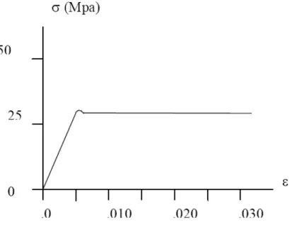
The cancellous bone tissue mechanical behaviour can be qualitatively represented as in Figure 14.

Figure 14 Compressive stress-strain curve for cancellous bone tissue

The compressive stress-strain curves of cancellous bone show an initial linear elastic region up to a strain of about 0.05. The material yielding occurs as the trabeculae begin to fracture. A plateau region of almost constant stress follows this initial elastic region until fracture, exhibiting a ductile material behaviour. After

yielding, it can sustain large deformations (up to 50% strain) while still maintaining its load-carrying capacity. Thus, trabecular bone can absorb substantial energy before mechanical failure. By contrast, cancellous bone fractures abruptly under tensile forces, showing a brittle material behaviour. The energy absorption capacity is considerably higher under compressive loads than under tensile loads.

Being a heterogeneous open cell porous solid, trabecular bone has anisotropic mechanical properties that depend on the porosity of the specimen as well as the architectural arrangement of the individual trabeculae. In order to specify its mechanical properties, one must therefore specify factors such as the anatomical site, loading direction with respect to the principal orientation of the trabeculae, age and health of the donor. Young’s module can vary 100-fold within a single epiphysis [16] and can vary on average by factor of three depending on loading direction [17,18]. Pathologies such as osteoporosis, osteoarthritis and bone cancer are known to affect mechanical properties [19,20]. Typically the modulus of human trabecular bone is in the range

(19)

- 18 -

0.010-2 GPa depending on the above factors. Strength, which is linearly and strongly correlated with modulus [16], is typically in the range 0.1-30 MPa [12].

(20)

1.1.3 References

1. Reilly DT and Burstein AH. The elastic and ultimate properties of compact bone tissue. J Biomech 1975; 8(6):393-405.

2. Ashman RB, Cowin SC, Van Buskirk WC, and Rice JC. A continuous wave technique for the measurement of the elastic properties of cortical bone. J Biomech 1984; 17(5):349-61. 3. Lakes RS and Katz JL. Viscoelastic properties of wet cortical bone--III. A non-linear

constitutive equation. J Biomech 1979; 12(9):689-98.

4. Carter DR and Caler WE. A cumulative damage model for bone fracture. J Orthop Res 1985; 3(1):84-90.

5. Currey JD. The effects of drying and re-wetting on some mechanical properties of cortical bone. J Biomech 1988; 21(5):439-41.

6. Sedlin ED. A rheologic model for cortical bone. A study of the physical properties of human femoral samples. Acta Orthop Scand 1965; :Suppl(83):1-77.

7. Lotz JC, Gerhart TN, and Hayes WC. Mechanical properties of metaphyseal bone in the proximal femur. J Biomech 1991; 24(5):317-29.

8. Bailey AJ, Wotton SF, Sims TJ, and Thompson PW. Biochemical changes in the collagen of human osteoporotic bone matrix. Connect Tissue Res 1993; 29(2):119-32.

9. Currey JD. Cortical Bone, in Handbook of Biomaterial Properties, J Black and G Hastings, Editors. 1998, Chapman&Hall: London, UK.3-14.

10. Carter DR and Caler WE. Cycle-dependent and time-dependent bone fracture with repeated loading. J Biomech Eng 1983; 105(2):166-70.

11. Keller TS. Predicting the compressive mechanical behavior of bone. J Biomech 1994; 27(9):1159.

12. Keaveny TM. Cancellous Bone, in Handbook of Biomaterial Properties, J Black and G Hastings, Editors. 1998, Chapman&Hall: London, UK.15-23.

13. Kuhn JL, Goldstein SA, Feldkamp LA, Goulet RW, and Jesion G. Evaluation of a

microcomputed tomography system to study trabecular bone structure. J Orthop Res 1990; 8(6):833-42.

14. Mosekilde L, Bentzen SM, Ortoft G, and Jorgensen J. The predictive value of quantitative computed tomography for vertebral body compressive strength and ash density. Bone 1989; 10(6):465-70.

15. Gong JK, Arnold JS, and Cohn SH. Composition of Trabecular and Cortical Bone. Anat Rec 1964; 149:325-31.

(21)

- 20 -

16. Goldstein SA, Wilson DL, Sonstegard DA, and Matthews LS. The mechanical properties of human tibial trabecular bone as a function of metaphyseal location. J Biomech 1983; 16(12):965. 17. Townsend PR, Raux P, Rose RM, Miegel RE, and Radin EL. The distribution and anisotropy of

the stiffness of cancellous bone in the human patella. J Biomech 1975; 8(6):363-7.

18. Linde F, Pongsoipetch B, Frich LH, and Hvid I. Three-axial strain controlled testing applied to bone specimens from the proximal tibial epiphysis. J Biomech 1990; 23(11):1167-72.

19. Pugh JW, Radin EL, and Rose RM. Quantitative studies of human subchondral cancellous bone. Its relationship to the state of its overlying cartilage. J Bone Joint Surg Am 1974; 56(2):313-21. 20. Hipp JA, Rosenberg AE, and Hayes WC. Mechanical properties of trabecular bone within and

(22)

1.2 LHDL project

This thesis was carried out as part of LTM research group activities within the Living Human Digital Library project (LHDL). Therefore this chapter will briefly present the LHDL project and related LTM responsibilities. It must to be mentioned that LHDL project is an executive part of the bigger Living Human Project (LHP).

The LHP aimed to create an in silico model of the human musculoskeletal apparatus able to predict how mechanical forces are exchanged internally and externally at any dimensional scale from the whole body down to the protein level. This goal has been pursued through the following steps:

- creation of a community of researchers interested in the project and in the idea of exchanging information, data and models to create a collectively owned resource - development and implementation of a specialized infrastructure, called the Living Human Digital Library (LHDL), which makes it possible for the community members to create, share, modify the data and modeling resources that constitute the LHP.

The LHDL involved various institutions, each contributing different skills (Fig.1).

The substance of the LHP and was biomechanical data, and therefore the data collection was a fundamental step of the LHDL project. Only two of LHDL project participants were involved in data collection. The ULB has granted two human cadavers, subjects to this functional-anatomical and multi-level study. The ULB has also provided all anatomical measurements, like whole body CT and MRI or passive kinematics.

(23)

- 22 -

Fig. 1. The structure of the Living Human Project and the participant institutions

Dissectioned bone segments were shipped to IOR for biomechanical investigations. The LTM laboratory consists of three subgroups: experimental, biological and computational which were subsequently investigating this same bone segments but at different levels. Once mechanically tested at the organ-level, bones were sectioned and the tissue-level biomechanical data were assessed, such as density, mineral content, micro hardness and Young’s modules. At last part the bones sections underwent biological study. Collagen orientation and non mineral content were investigated. Simultaneously computational models, based on CT and experimental data, were created.

This thesis was dedicated to cover the organ-level experimental investigation part and its aims will be presented in the next chapter.

(24)

1.3 Scope of the thesis

The biomechanical in vitro investigation of human long bones was a general aim of this work. However this complex task consisted of well defined specific goals which shall be listed at this point. The partial scopes can be divided into:

Methodology related:

1. First scope was to create a marker system for different medical imaging techniques. The LHDL principal requirement was that all measurements acquired at different levels of the same cadavers become set together within univocal coordinate system. However, until now there wasn’t a marker suitable for each of the visualisation techniques and preventing bones damaging from drilling holes for marker fixation in this same time (not magnetic- MRI, no artefacts-CT, not bone damaging- in-vitro testing).

2. The second scope within this thesis was to compare three anatomical coordinate systems for the tibia-fibula complex. The importance of this study lays at defending the most repeatable technique for tracing anatomical planes and subsequently to provide the best matching for multi level data testing.

3. Third scope was to create testing device able to accurately determine the position of the applied force during in-vitro tests. This is of great importance for subject-specific FE-models validation, which are extremely sensitive to theirs boundary conditions.

4. The forth scope of this thesis was to create a novel measuring technique to measure able to distinguish the crack initiation point on a bone surface when tested to fracture. This technique had to provide higher spatial resolution than high speed cameras techniques does.

Data collection related:

1. First of all, the LHDL project was aimed at collection of an enormous, encyclopaedic biomechanical dataset. A general biomechanical properties, such as whole bone stiffness strength and strain distribution of all major six human long

(25)

- 24 -

bones (radius, ulna, humerus, femur, tibia and fibula) had to be acquired. Moreover a loading direction and loading velocity influence had to be evaluated.

2. Secondary goals, the specific research questions, were related to the proximal portion of the femur. First study was aimed to provide a better understanding of the strain distribution, and of its correlation with the different directions of loading, and with bone quality. Where the second study, was aimed to investigate how to replicate in-vitro clinically relevant proximal femoral fractures.

(26)

1.4 Structure of the thesis

The present thesis consists of nine studies developed in the LTM during the LHDL project. Six of those studies have become articles. Three papers have been already published, two on the Journal of Biomechanics one on Strain, and three have been submitted.

Three other studies are not published, however they were technically essential to the development of the project and therefore have been presented here.

In the following paragraphs a path, created to guide trough the present thesis and to bring forward the role of the author of this thesis has been presented.

Section Methodology, contains four chapters introducing technical requirements essential to compete experimental measurements.

Chapter 2.1, “The marker system for different medical imaging techniques”, describes development of tool able to assist data collection for different investigations at different levels: whole-body, body-segments and organs with this same univocal reference system. The entire study was developed by the author and partially carried out at the Department of Anatomy, Université Libre de Bruxelles, Belgium.

Chapter 2.2, “Comparison of three anatomical coordinate systems for tibia-fibula complex”. Whereas the procedure for defining of anatomical plans for femur has been well defined and validated, such verification was missing for tibia-fibula complex. Therefore the LTM group compared three different anatomical coordinate systems to define the most reproducible and the simples for the experimental applications.

Once univocal reference system was ensured for both whole body and bone segment level, a testing setup had to be projected and developed. The experimental setup for whole bones testing had to provide all the FEM related constrains such as force, displacement, strain. However the load direction and fracture initiation point were difficult to assess.

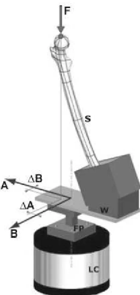
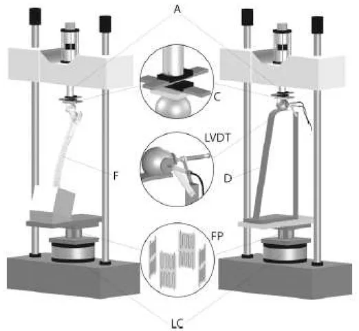
Chapter 2.3 “A Method to Improve Experimental Validation of Finite-Element Models of Long Bones” presents development of a load cell (called FP-transducer) able to reproduce the position of the applied force during an in vitro test, where the

(27)

- 26 -

resultant joint force is one of boundary conditions crucial for accurate validation of FE-models.

Chapter 2.4 “A new technique for bone crack propagation registration” presents a novel technique for registration of fractures called the Crack-Grid. The main purpose of developing this technique was to distinguish crack initiation point, with the spatial resolution better than this given by the high speed camera. Providing accurate data for the FEM validation and delivering an extra information related to bone structure mechanics during bone fracture tests. Moreover thanks to its performances (700kHz sampling rate, 3mm spatial resolution, easy application onto irregular surfaces) and relatively low cost (<€100) this technique can find an application in other fields of materials science.

Section “General biomechanical characterization of long bones”, has been dedicated to present results related to general bone structural biomechanics such as whole bone strain distribution, whole bone stiffens, and whole bone strength.

Chapter 3.1, “LHDL related data acquisition”, summarises all tests executed within the LHDL project and related results, for both cadavers. The author was responsible for preparation and execution of all tests. A complete dataset contains: a strain-distribution, stiffness and strength information for each tested bone segment and has been already shared trough the dedicated internet infrastructure www.biomedtown.org.

Basing on the LHDL data, collected by the author, a specific study has been carried out. Chapter 3.2, “Structural behaviour of the long bones of the human lower limbs”, deals with two experimental factors: loading direction and loading velocity. By comparing these factors, an insight has been given into the understanding of the bone-structure viscoelastic behaviour within physiological strain rates.

In the section “Specific biomechanical characterization of long bones” have been presented two studies concerning a human proximal femoral metaphysis. These studies were carried out on femoral bones which were not a part of the LHDL project and results were not directly related to the dataset requested for the LHDL. However results of these studies have been a support to the computational studies carried out at LTM

(28)

within the project. Moreover these same experimental setups and techniques developed within the LHDL project were applied here.

Chapter 4.1 “Strain distribution in the proximal human femoral metaphysis” describes a detailed, strain-gauge based, study. The strain distribution was correlated with the different directions of loading and with bone quality. To provide a better understanding of the proximal femur metaphysis stress/strain state has been of great interest because of its relevance for hip fractures and prosthetic replacements.

Spontaneous fractures are representing a significant percentage of proximal femur fractures. However this type of fracture has seldom been investigated and there is no evidence, nor consensus on the most relevant loading scenario. Chapter 4.2 “In vitro replication of spontaneous fractures of the proximal human femur” presents combined experimental/computational study aimed to develop and validate an experimental method to replicate spontaneous fractures in vitro, basing on clinically relevant loading scenario.

The know-how developed about testing the proximal femur was applied to testing and optimizing proximal epiphyseal replacement of the femur. In Appendix, the paper “Stress-shielding and stress-concentration of contemporary epiphyseal hip prostheses” has been presented.

(29)

- 28 -

(30)

2.1. The marker for multi biomedical visualisation

Modeling of musculo-skeletal system is currently challenging due to the Inhomogeneity across the different multi-scale levels and the mis-match between the different data sets obtained. Thus, limiting the accuracy of the models in turn limiting the conclusions that can be drawn both in terms of basic scientific principle sand within a more applied clinical context. The current state-of-the-art in the modeling field reports the use of data obtained from various sources (e.g. literature, colleagues, the Internet) without clear links between these sources and often lacking in validation (e.g. as done by Refs?). This LHDL project, however, aimed to obtain mutli-scale data that was self-consistent, by obtaining all data from the same cadaver using the same univocal reference system. Thus, correcting the ad-hoc approach used so far for such data collection.

To provide this reference system dedicated markers were crafted. Suitable for each particular biomedical visualization technique (CT, MRI and stereophotogrammetry) and with respect to specific constrains. The entire study was carried out by the author and partially carried out at the Department of Anatomy, Université Libre de Bruxelles, Belgium.

During the designing process several constrains were considered:

- Constraint 1. Following recommendations from a feasibility study (performed before

the LHDL project), the technical frames including reflective markers were mounted on customized pins allowing easy setting and removing. A special interface between the pin and the technical frame was required to maintain a constant position and orientation between the two components relative to each other . Technical frames were removed before storage in order to reduce (taking it out of the cooling room where it was kept between two dissection, setting the specimen on the experimental jig, dissection of the specimen, etc) reduce the likelihood of collisions with the technical frames which would displace them . This would have lead to a lost of the relationship between the frame and the underlying bony structure.

Constraint 2. Latter stage of the LHDL data collection protocol included analysis of

(31)

- 30 -

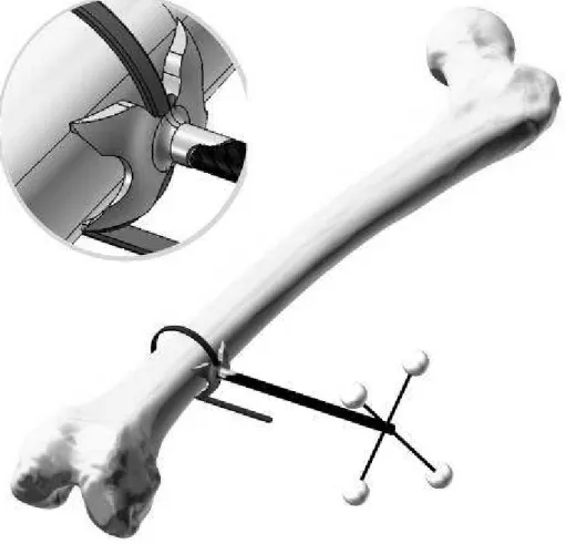
therefore impossible to drill the pins used to support the above technical frames into some bones (mainly long bones: humerus, clavicles, femurs, tibias, ulnas, radiuses, and sternum). Therefore the basis of the technical frame included a hole. A plastic strap that was wrapped around the diaphysis of long bones, was present inside this hole, in such a way that the technical frame and its basis were “firmly” linked to the bone of interest (Fig1). Other bones (skull, jaw, scapula, iliac bones, metacarpal bones, metatarsal bones) were drilled to enable their attachment to the external frames.

Figure 1 Model of the femur with the marker and close-up of the fastening strap

Constraint 3. In terms of the visualization techniques, the technical requirements for

usage of each include:

- CT-scan is used not only for general skeleton morphology visualization. Material properties of bone are derived from image gray-scales, following calibration, for future subject specific FE-models. Therefore marker pins and supports were made of carbon-fiber and aluminum (materials less or equally dense as bone) in order to avoid imaging artifacts.

(32)

- MRI requires usage of non ferromagnetic materials. And carbon fiber and aluminum are suitable.

In summary, markers met considered requirements contributing to the multi level data collection. The data collection of both cadavers was as follows: The cadaver of a donor with average morphology from the ULB donation program was used. Each body

segment (thighs, shanks, feet, forearms, etc) was equipped with reflective markers to create technical frames linked to all major segment bones within 3 different visualization techniques. These reflective markers were visible within CT-scan datasets, stereophotogrammetry used to digitize dissection results, and stereophotogrammetry used for motion analysis.

(33)

- 32 -

2.2 Comparison of three standard anatomical

reference frames for the tibia-fibula complex

Giorgia Conti, MEng 1, 2, Luca Cristofolini, PhD 1, 2, Mateusz Juszczyk, MEng 1, 2, Alberto Leardini, PhD 3, Marco Viceconti, PhD 1

1

Laboratorio di Tecnologia Medica, Istituto Ortopedico Rizzoli, Bologna, Italy

2

Engineering Faculty, University of Bologna, Italy

3

Laboratorio di Analisi del Movimento, Istituto Ortopedico Rizzoli, Bologna, Italy

The author contributed to this study at projecting experimental setup and executing measurements. This study was published on Journal of Biomechanics.

(34)

2.2.1 Abstract

Definition of anatomical reference frames is necessary both for in vitro biomechanical testing, and for in vivo human movement analyses. Different reference frames have been proposed in the literature for the lower limb, and in particular for the tibia-fibula complex. The scope of this work was to compare the three most commonly referred proposals (proposed by Ruff et al 1983, by Cappozzo et al 1995, and by the Standardization and Terminology Committee of the International Society of Biomechanics, Wu et al. 2002). These three frames were identified on six cadaveric tibia-fibula specimens based on the relevant anatomical landmarks, using a high-precision digitizer. The intra-operator (ten repetitions) and inter-operator (three operators) repeatability were investigated in terms of reference frame orientation. The three frames had similar intra-operator repeatability. The reference frame proposed by Ruff et al had a better inter-operator repeatability (this must be put in relation with the original context of interest, i.e. in vitro measurements on dissected bones). The reference frames proposed by Ruff et al and by ISB had a similar alignment; the frame proposed by Cappozzo et al was considerably externally rotated and flexed with respect to the other two. Thus, the reference frame proposed by Ruff et al is preferable when the full bone surface is accessible (typically during in vitro tests). Conversely, no advantage in terms of repeatability seems to exist between the reference frames proposed by Cappozzo et al and ISB.

Keywords:

Shank coordinate system, tibia-fibula complex, anatomical reference frames, in vitro landmarks, in vivo human movement analysis

(35)

- 34 -

2.2.2. INTRODUCTION

Univocal definition of reference frames is extremely important in musculoskeletal biomechanics (Fung, 1980; Currey, 1982; Van Sint Jan and Della Croce, 2005). In in

vivo motion analysis, reference frames enable tracking segment and joint motion, and

calculation of joint moments (Cappozzo et al., 1995; Wu et al., 2002). Reference frames in vitro enable aligning correctly the specimens and the test loads, and defining testing conditions so that these can be replicated (O'Connor, 1992; Cristofolini, 1997). This applies to all lower limb segments. Whereas a number of definitions have been discussed for the femur (Della Croce et al., 2003), little has been reported for the tibia-fibula complex.

One of the first reference frames for the lower limb bones was proposed by (Ruff, 1981; Ruff and Hayes, 1983). This frame was based on identification of landmarks and geometrical measurements that are possible only in vitro on dissected femur and tibia segments (further details in Materials and Methods). Although this method was originally intended for anatomical analyses, it was adopted successfully for in vitro biomechanical tests both on the femur (Cristofolini, 1997) and tibia (Cristofolini and Viceconti, 2000; Heiner and Brown, 2001; Gray et al., 2007; Gray et al., 2008). A different anatomical reference frame was proposed by (Cappozzo, et al., 1995) to provide consistent identification of landmarks for a more repeatable motion analysis. As it was intended for routine clinical use, it was based on palpation of those anatomical landmarks than can be accessed non-invasively in vivo (further details in Materials and Methods). Original identification of bony prominences rather than anatomical planes and axes lead to more repeatable measurements in gait analysis (Leardini et al., 2007). Later, the Standardization and Terminology Committee of the International Society of Biomechanics (ISB) proposed a slightly different reference frame (Wu, et al., 2002) (further details in Materials and Methods). Although such frame was mainly defined for movement analysis, this was the first time that the need for combining in vitro and in vivo reference frames was considered.

It is clear that an ideal reference frame should be based on landmarks that are easily and reproducibly identified in all subjects, also in case of severe bone deformity. Serious implications of incorrect identification of landmarks and reference frames have been reported both in vitro (Cristofolini and Viceconti, 2000; Gray, et al., 2007), and

(36)

in vivo (Della Croce et al., 2005; Thewlis et al., 2008). However, the repeatability in

identifying these three reference frames (Ruff and Hayes, 1983; Cappozzo, et al., 1995; Wu, et al., 2002) for the tibia-fibula complex has never been reported. Also, as such reference frames were defined independently from each other, the relative orientation of one system respect to the other is unknown.

The scope of this work was to compare these three reference frames for the tibia-fibula complex (Ruff and Hayes, 1983; Cappozzo, et al., 1995; Wu, et al., 2002), with the following goals:

• Assess the intra-operator repeatability (i.e. when the same operator repeatedly identifies the reference frame on the same specimen);

• Assess the inter-operator repeatability (i.e. when the different operators identify the reference frame on the same specimen);

• Assess if the three reference frames overlap and, if not, to assess the relative poses.

2.2.3 MATERIALS AND METHODS

2.2.3.1 Specimens

Six specimens, consisting of intact tibia-fibula complexes were obtained through international donation programs from donors free of any musculoskeletal pathologies (Table 1). They were visually inspected and CT-scanned (HiSpeed, General Electric, USA) to document bone quality and lack of abnormality or defects. All soft tissues were removed, leaving only the articular cartilages and the interosseous membrane. The ligaments of the proximal and distal tibiofibular articulations (syndesmosis) were left intact to preserve the original relative position and orientation. To avoid errors due to bone shrinkage, tissue hydration was preserved by means of cloths soaked with saline solution during the measurement sessions.

Table 1 – Details of the sample analyzed (average, standard deviation and range over the 6 specimens). The ‘biomechanical length’ of the tibia (BL, see also Fig. 1) as in (Ruff and Hayes, 1983), is reported in the first column. Donors’ details are summarized in the last four columns.

Biomech length BL (mm) Donor’s side Age at death (years) Donors’ height (cm) Body Mass Index, BMI, (kg/m2) Gender

(37)

- 36 - Average ±±±± standard deviation 358 ± 12.6 56 ± 23.6 173 ± 10.7 21 ± 3.7 Range 341 to 379 50% right 50% left _{27 to 79} _{165 to 191} _{16.7 to 24.1} 50% male 50% female

2.2.2.3.2 Definition of the three reference frames

The reference frame Ruff-coord (Fig. 1) proposed by (Ruff, 1981; Ruff and Hayes, 1983) is based on the centers of the articulating cartilage areas at the proximal and distal tibia, with no landmarks on the fibula. Such centers must be measured using calipers. The Ruff-coord can only be identified in vitro, when the bone surface is visible. It must be noted that Ruff-coord only relies on the tibial anatomy, while the fibula is ignored. As (Ruff, 1981; Ruff and Hayes, 1983) did not suggest a separate reference for the fibula, we propose to use the same reference frame for the entire tibia-fibula complex.

Fig. 1 – Reference frame Ruff-coord (Ruff, 1981; Ruff and Hayes, 1983) for a right tibia-fibula complex: anterior view (a), transverse view from above (b) and transverse view from below (c). The centers of the two tibial condyles (MTC, LTC) and of the surface articulating with top of the talus (TAS) are initially identified. This is performed by locating (with calipers) the mid-points in the antero-posterior and medio-lateral directions on each cartilage surface (as this procedure relies on an estimated

(38)

provisional alignment, the procedure must be iteratively repeated –typically twice- until no significant further correction is needed). As an example, the location of TAS is shown in (c). The midpoint (MP) between the two tibial condyles center points (MTC and LTC) is then calculated. The frontal plane is the one passing through MTC, LTC and TAS; the sagittal plane is perpendicular to the frontal plane and goes through points MP and TAS.

The reference frame Cappozzo-coord (Fig. 2) proposed by (Cappozzo, et al., 1995) is based on landmarks of the tibia and fibula that need to be palpable also in vivo. The reference frame ISB-coord (Fig. 3) recommended by the ISB (Wu, et al., 2002) is based on the same landmarks as Cappozzo-coord distally, but on different landmarks proximally (with landmarks over only the tibial plateau).

Fig. 2 – Reference frame Cappozzo-coord (Cappozzo, et al., 1995) for a right tibia-fibula complex (anterior view). First, the tibial tuberosity (TT), the apex of the head of the fibula (HF), the distal apex of the medial and lateral malleoli (MM, LM) are identified. The midpoint (MPM) of the line joining MM and LM is then calculated (this point coincides with IM of Fig. 3 (Wu, et al., 2002)). The frontal plane passes through HF, LM and MM; the sagittal plane is perpendicular to the frontal plane and goes through points MPM and TT

(39)

- 38 -

Fig. 3 – Reference frame ISB-coord proposed by the Standardization and Terminology Committee of the International Society of Biomechanics (Wu, et al., 2002) for a right tibia-fibula complex (anterior view). First, the most medial and lateral points on the edge of the relevant condyles (MC, LC), the tip of the medial and lateral malleoli (MM, LM) are identified. The inter-malleolar point (IM, which coincides with MPM of Fig. 2 (Cappozzo, et al., 1995)) located midway between MM and LM and the inter-condylar point (IC) located midway between the MC and LC are calculated. The frontal plane passes through IM, MC and LC; the sagittal plane is perpendicular to the frontal plane and containing the points IC and IM.

Both Cappozzo-coord and ISB-coord rely on the anatomy of the entire tibia-fibula complex. It must be stressed that the Cappozzo-reference and the ISB-reference are designed for in vivo use, and the landmarks are identified with some approximation because of the interposition of soft tissues. In this study all the landmarks were accessed directly on the bone surfaces.

Relative orientation for each pair of reference frames was expressed using the same approach used by (Grood and Suntay, 1983) for referring one anatomical segment to the other. This entails defining flexion/extension as the relative orientation about the medio-lateral axis of a first frame, internal/external rotation as the relative orientation about the vertical axis of the second frame, and abduction/adduction as the relative orientation about a ‘floating’ axis orthogonal to the previous two.

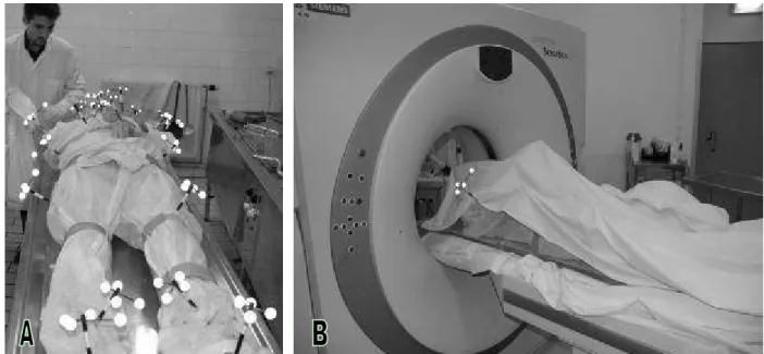
2.2.3.3 In vitro acquisition

The landmarks described above were acquired with a 3D digitizer (Mod. Gage-Plus-V1.5, Faro-Europe, Stuttgart-Weilimdorf, Germany) with an accuracy of 10 micron.

(40)

The specimens were held in space by an adjustable vice. From these landmarks, the position and orientation of the three reference frames (Ruff-coord, Cappozzo-coord,

ISB-coord) was obtained for each specimen. Reference frames belonging to left

specimens were mirrored so as to treat them all as right.

To assess the intra-operator repeatability, each reference frame was identified ten times by the same operator on one randomly selected specimen, at a time distance of 10-20 minutes. To assess the inter-operator repeatability, three operators with a good knowledge of musculoskeletal biomechanics were asked to identify the landmarks of the three reference frames on each specimen. To avoid conditioning or biasing between replicates and between operators, each acquisition was blinded with respect to previous ones: the landmarks were only temporarily marked on the bone, and erased before each new acquisition.

2.2.3.4 Statistical analysis

The orientation of each reference frame and of each repetition was expressed using the angles defined by (Grood and Suntay, 1983), using custom-written code in Matlab (Matlab inc, Natick, MA, USA).

To estimate the intra-operator repeatability (ten repetitions, one operator, one specimen):

• The average coordinates of each landmark (with respect to the digitizer coordinate system) was computed over the ten repetitions by the same operator;

• An average reference frame was identified based on such average landmarks; • The pose (i.e. of the angles defined by (Grood and Suntay, 1983)) of each of the

ten repetitions was computed with respect to such average reference frame;

• The variance and standard deviation of the ten poses (i.e. of the angles defined by (Grood and Suntay, 1983)) was computed;

• To compare the intra-operator repeatability of the three reference frames, an F-test was applied to the ratio of the respective variances.

To estimate the inter-operator repeatability (three operators, six specimens):

• For each specimen, the average coordinates of each landmark (with respect to the digitizer coordinate system) was computed between the three operators;

(41)

- 40 -

• For each specimen, an average reference frame was identified based on such average landmarks;

• For each operator, the pose (i.e. of the angles defined by (Grood and Suntay, 1983)) was computed with respect to such average reference frame, for each specimen;

• The variance and standard deviation of the ten poses (i.e. of the angles defined by (Grood and Suntay, 1983)) was computed, for each specimen;

• The Root Mean Square Error (RMSE) was computed between specimens;

• To compare the inter-operator repeatability of the three reference frames, an F-test was applied to the ratio of the respective variances.

To estimate the relative orientation of the three reference frames using a pairwise comparison of each reference frame with respect to the other:

• For each specimen, the average coordinates of each landmark (with respect to the digitizer coordinate system) was computed between the three operators, for each reference frame (Ruff-coord, Cappozzo-coord, ISB-coord);

• For each specimen, an average reference frame was identified based on such average landmarks, for each reference frame (Ruff-coord, Cappozzo-coord,

ISB-coord);

• The relative orientation of each reference frame respect to the each of the other two frames was computed, for each specimen: Cappozzo-coord with respect to

Ruff-coord, Ruff-coord with respect to ISB-Ruff-coord, ISB-coord with respect to Cappozzo-coord;

• The average and standard deviation of such relative orientations was computed between specimens;

• The significance of such relative orientations (Cappozzo-coord with respect to

Ruff-coord, Ruff-coord with respect to ISB-coord, ISB-coord with respect to Cappozzo-coord) was assessed with two-tailed paired t-tests.

(42)

2.2.4 RESULTS

2.2.4.1 Repeatability of the landmarks

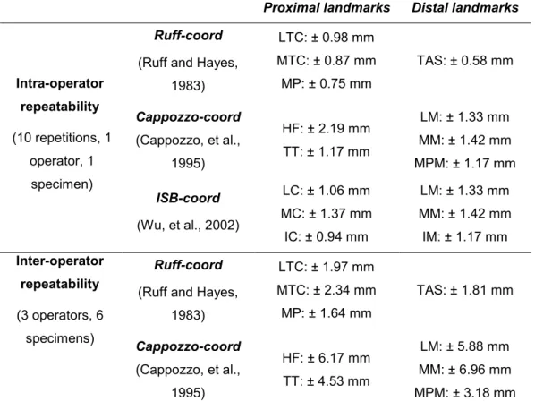
For Ruff-coord the intra-operator repeatability in identifying the individual landmarks was 0.58-0.98 mm (the error was largest for the center of the tibial condyles, MTC and LTC, Table 2); the inter-operator repeatability was 1.64-2.34 mm (the error was largest for the center of the tibial condyles, MTC and LTC). For Cappozzo-coord the intra-operator repeatability for the landmarks was 1.17-2.19 mm (the error was largest for the head of the fibula, HF, Table 2); the inter-operator repeatability was 3.18-6.96 mm (the error was largest for MM, LM and HF). For ISB-coord the intra-operator repeatability for the landmarks was 0.94-1.42 mm (the error was similar for all landmarks, Table 2); the inter-operator repeatability was 3.18-7.07 mm (the error was largest for the most medial point on the tibial condyles, MC, and for the medial malleolus, MM).

Table 2 – Repeatability (vector error) of the identification of the landmarks defined for the three reference frames examined. Landmarks are defined as in Fig. 1 (Ruff-coord), Fig. 2 (Cappozzo-coord) and Fig. 3 (ISB-coord).

Proximal landmarks Distal landmarks Ruff-coord

(Ruff and Hayes, 1983) LTC: ± 0.98 mm MTC: ± 0.87 mm MP: ± 0.75 mm TAS: ± 0.58 mm Cappozzo-coord (Cappozzo, et al., 1995) HF: ± 2.19 mm TT: ± 1.17 mm LM: ± 1.33 mm MM: ± 1.42 mm MPM: ± 1.17 mm Intra-operator repeatability (10 repetitions, 1 operator, 1 specimen) ISB-coord (Wu, et al., 2002) LC: ± 1.06 mm MC: ± 1.37 mm IC: ± 0.94 mm LM: ± 1.33 mm MM: ± 1.42 mm IM: ± 1.17 mm Ruff-coord

(Ruff and Hayes, 1983) LTC: ± 1.97 mm MTC: ± 2.34 mm MP: ± 1.64 mm TAS: ± 1.81 mm Inter-operator repeatability (3 operators, 6 specimens) Cappozzo-coord (Cappozzo, et al., 1995) HF: ± 6.17 mm TT: ± 4.53 mm LM: ± 5.88 mm MM: ± 6.96 mm MPM: ± 3.18 mm

(43)

- 42 - ISB-coord (Wu, et al., 2002) LC: ± 5.62 mm MC: ± 7.07 mm IC: ± 3.70 mm LM: ± 5.88 mm MM: ± 6.96 mm IM: ± 3.18 mm

2.2.4.2 Repeatability of the reference frames

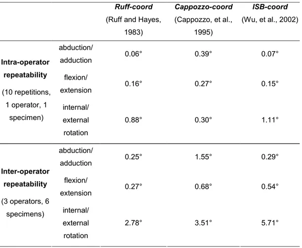
The intra-operator repeatability was of the same order of magnitude for the three reference frames (Table 3).

Table 3 – Repeatability of the definition of the three reference frames examined for the tibia-fibula complex.

Ruff-coord

(Ruff and Hayes, 1983) Cappozzo-coord (Cappozzo, et al., 1995) ISB-coord (Wu, et al., 2002) abduction/ adduction 0.06° 0.39° 0.07° flexion/ extension 0.16° 0.27° 0.15° Intra-operator repeatability (10 repetitions, 1 operator, 1 specimen) internal/ external rotation 0.88° 0.30° 1.11° abduction/ adduction 0.25° 1.55° 0.29° flexion/ extension 0.27° 0.68° 0.54° Inter-operator repeatability (3 operators, 6 specimens) internal/ external rotation 2.78° 3.51° 5.71°

In abduction/adduction Cappozzo-coord was significantly less repeatable than

Ruff-coord and ISB-Ruff-coord (F-test, p<0.00005); the difference between the repeatability of Ruff-coord and ISB-coord was not significant (F-test, p=0.7). The repeatability was

similar (F-test, p>0.1) for the three reference frames in flexion/extension. In internal/external rotation Cappozzo-coord was more repeatable than Ruff-coord and

(44)

ISB-coord (F-test, p<0.005); the difference between the repeatability of Ruff-coord and ISB-coord was not significant (F-test, p=0.5).

The inter-operator repeatability of the reference frames was worse than the intra-operator repeatability (Table 3). In the frontal plane (abduction/adduction)

Cappozzo-coord was one order of magnitude less repeatable than Ruff-Cappozzo-coord and ISB-Cappozzo-coord

(F-test, p<0.0001); the difference between Ruff-coord and ISB-coord was not significant (F-test, p=0.3). In the sagittal plane (flexion/extension) Ruff-coord was more repeatable than Cappozzo-coord and ISB-coord (F-test, p<0.01); the difference between Cappozzo-coord and ISB-coord was not significant (F-test, p=0.3). In the transverse plane (internal/external rotation) the only significant difference was that

Ruff-coord was more repeatable than ISB-coord (F-test, p<0.01); all other differences

were not significant (F-test, p>0.05).

2.2.4.3 Different orientation of the reference frames

The most obvious difference was the external rotation of Cappozzo-coord with respect to the other two reference frames (Fig. 4 and Table 4).

Table 4 – Relative orientation of the three reference frames using a pairwise comparison of each reference frame with respect to the other (see also Fig. 4). (*) tailed paired t-test: p<0.05, (**) two-tailed paired t-test: p<0.005

Pairs of reference frames being compared Rotations of Cappozzo-coord (Cappozzo, et al., 1995) respect to

Ruff-coord (Ruff and

Hayes, 1983)

Rotations of

Ruff-coord (Ruff and

Hayes, 1983) respect to ISB-coord (Wu, et

al., 2002)

Rotations of

ISB-coord (Wu, et al.,

2002) respect to Cappozzo-coord (Cappozzo, et al., 1995) abduction/ adduction abducted by <1° adducted by <1° abducted by <1° flexion/ extension flexed by 4° (*) flexed by <1° extended by 3° (*) internal/ external rotation externally rotated by 39° (**) externally rotated by 4° internally rotated by 34° (**)

This is accounted for by the definition of the frontal plane of Cappozzo-coord, which includes the two apexes of the malleoli, being the lateral malleolus much more posterior than the medial one. No significant difference (paired t-test, p>0.2) existed between the pose of Ruff-coord and ISB-coord (Fig. 4 and Table 4). Cappozzo-coord

(45)

- 44 -

was significantly flexed (paired t-test, p=0.006) and externally rotated (paired t-test, p=0.002) with respect to ISB-coord. Cappozzo-coord was significantly flexed (paired t-test, p=0.02) and externally rotated (paired t-test, p=0.002) with respect to

Ruff-coord. The fact that the two malleoli (used in Cappozzo-coord) are more posterior than

the points on the tibial tray identified by Ruff-coord and ISB-coord explains such differences.

Fig. 4 – Alignments of the three reference frames on a right tibia-fibula complex in an antero-lateral view. The three frames had similar alignments in the sagittal and transverse planes. However,

Cappozzo-coord was translated laterally and externally rotated with respect to Ruff-coord in the frontal

plane. No significant rotation existed between Ruff-coord and ISB-coord. Relative orientations are detailed in Table 4.