3D-printed trabecular bone : role of the microarchitecture on bone mechanical behaviour

1

SCHOOL OF INDUSTRIAL AND INFORMATION ENGINEERING Master of Science in Materials Engineering and Nanotechnology

3D-printed trabecular bone:

role of the microarchitecture on bone

mechanical behaviour

Supervisor

Prof. Laura VERGANI

Co-Supervisor

Prof Flavia LIBONATI Ph.D. Federica BUCCINO

Candidates

Isabella BRAMATI – 905289 Chiara COPELLI – 893858 Academic Year 2020 – 2021

II

This thesis is the result of many efforts that required the cooperation of several people who we would like to thank. We are deeply grateful to Prof. Laura Vergani and Prof Flavia Libonati for giving us the opportunity to participate in this intriguing research. We would like to thank Eng. Federica Buccino for patiently guiding us in all stages of the work.

And last but not least, a double thanks to our friends and family who have supported and encouraged us during this six-year experience.

III Osteoporosis is a bone disease, characterized by bone tissue loss, bone microarchitecture deterioration and, consequently, bone strength reduction. Vertebral fracture is one of the most common types of fracture that usually affects elderly people. Several studies have already pointed out how the micro-architecture impacts the mechanical properties.

In this thesis work, the aim is to elucidate the role of the microarchitecture on the overall mechanical properties by means of mechanical testing, image analyses and numerical simulations of 3D-printed trabecular bone replicas. The use of additive manufacturing allows to overcome the material influence, focusing only on the trabecular bone network. The 3D-printed (3DP) polymeric samples replicating trabecular porcine bone were used. A Micro-computed tomography (Micro-CT) scan was carried out in order to obtain cross-sectional images of the 3DP samples, necessary for the morphological parameters computation and for the development of finite element models (FEM).

The first part of the study presents a comparison between the morphological parameters of the original and the polymeric specimens. The Volume Fraction (BV/TV) and the Degree of anisotropy (DA) were the chosen parameters because, together, they explain about 90% of the variation in trabecular bone tissue elastic properties. Subsequently, static uniaxial compression tests were experimentally carried out on the samples and the apparent elastic modulus was determined. Among all the bone replicas, two samples were selected for the development of the finite element models.

The FE-simulations of the samples (i.e. global model) allowed to locate the region characterized by the highest minimum principal strain (in absolute value) where failure is likely to occur. A first sub-region is selected, to develop a local model called failure band model. Then, from this region, the most critical zone is chosen to develop another sub-model, called Representative Volume Element (RVE) model.

IV Keywords: porcine vertebra, trabecular bone micro-architecture, micro-CT, 3D printing, FEM

V L’osteoporosi è una malattia ossea caratterizzata dal deterioramento della struttura ossea e conseguente riduzione della sua resistenza. Inparticolare le fratture vertebrali risultano le più diffuse, con un incidenza elevata nella popolazione femminile di età superiore a 80 anni.

In questo lavoro di tesi, l’obiettivo è quello di sottolineare il ruolo della microstruttura sulle proprietà meccaniche attraverso test meccanici, analisi di immagini e simulazioni numeriche eseguite su repliche di provini di osso trabecolare, stampate mediante tecniche di 3D printing. L’utilizzo dell’additive manufacturing permette di isolare la morfologia ossea, al fine di studiarne l’influenza sul comportamento meccanico del materiale. Sono stati utilizzate delle repliche in materiale polimerico di provini di ossa trabecolari, provenienti da vertebre porcine. Una scansione dei provini 3D tramite Micro-CT permette di ottenere le informazioni necessarie per il calcolo dei parametri morfologici e per la realizzazione di modelli ad elementi finiti (FEM).

La prima parte dello studio presenta un confronto tra i parametri morfologici originali e quelli dei provini stampati. I parametri di confronto scelti sono: la frazione volumetrica (BV/TV) e il grado di anisotropia (DA): essi, infatti, spiegano circa il 90% delle variazioni delle proprietà elastiche del tessuto trabecolare osseo. In seguito, sono stati eseguiti dei test uniassiali a compressione statica, attraverso i quali è stato calcolato il modulo elastico apparente di ciascun provino. Tra tutte le repliche stampate 3D, sono stati scelti 2 provini per lo sviluppo dei modelli ad elementi finiti. Queste simulazioni, eseguite sull’intero provino (modello globale), permettono di individuare la zona caratterizzata dal più alto valore di minima deformazione principale, in valore assoluto. Tale criterio è stato scelto in quanto l’osso si deforma plasticamente a deformazioni approssimabili come isotropiche, nonostante la sua natura anisotropica, pertanto, rispetto a criteri basati sullo sforzo, è più semplice e accurato. Partendo dal modello globale, è stata selezionata una sotto-regione per

VI ulteriore sotto-modello, chiamato Representative Volume Element (RVE). Il RVE aiuta ad identificare più accuratamente la trabecola soggetta alla deformazione più elevata e dunque probabile sito di inizio del danneggiamento.

Parole chiave: vertebra suina, microarchitettura dell’osso trabecolare, Micro-CT, stampa 3D, FEM

VII 2.1 Bone microarchitecture ... 2 2.1.1 Rode-like trabeculae ... 5 2.1.2 Plate-like trabeculae: ... 6 2.2 Clinical Parameters ... 7 2.3 Morphological parameters ... 10

2.4 Microarchitecture visualization through the Micro-CT ... 13

2.5 Finite Element Models ... 14

2.6 Additive manufacturing for bone studies ... 18

2.8 General objectives ... 21

3.1 EXPERIMENTAL SECTION ... 22

3.1.1 Original porcine samples ... 23

3.1.2 3D printing ... 24

3.1.3 Scanning Procedure: Micro-CT ... 26

3.1.4 Image analysis ... 28

3.1.5 Mechanical tests ... 34

3.2 COMPUTATIONAL SECTION ... 36

3.2.1 Finite Element Models ... 36

3.2.2 Validation of the models ... 39

3.2.3 From Global Model to sub-models ... 41

3.2.4 Failure Band Model ... 42

VIII

4.1.2 Morphological parameters discussion ... 55

4.1.3 Compression tests results ... 64

4.1.4 Compression test discussion ... 68

4.2 COMPUTATIONAL SECTION ... 74

4.2.1 Global model validation ... 75

4.2.2 Validation discussion ... 78

4.2.3 From global model to sub-models results ... 81

IX Figure 1.1 Comparison between healthy vertebral bone (left) and osteoporotic one (right). Adapted

from [1] ... 1

Figure 1.2 Age-specific and sex specific incidence of osteoporotic fractures on the right, projected costs of osteoporotic fractures (adapted from [4]) ... 2

Figure 2.1 Bone main features ... 2

Figure 2.2 Distribution of spinal loads on the anterior and posterior weight-bearing columns in a normal lumbar spine (A). Shifting of spinal loads to the posterior column after degenerative pathology to the lumbar spine (B). ... 3

Figure 2.3 Summary of bone architecture ... 5

Figure 2.4 Rode-like structure [17] ... 6

Figure 2.5 Plate-like structure [17] ... 6

Figure 2.6 DXA comparison between an healthy bone on the left and an onsteoporotic one on the right, adapted from [23] ... 8

Figure 2.7 Healthy bone on the left and osteoporitic one on the right ... 8

Figure 2.8 Numerical data of Micro-CT studies of vertebrae, adapted from [28] ... 11

Figure 2.9 Summary of clinical, morphological and numerical parameters for bone assessment ... 12

Figure 2.10 Bone scale of observations, adaptated from [35] ... 14

Figure 2.11 FE simulations of cubic lattices with increasing disorder (from left ro right) ... 15

Figure 2.12 Femoral head specimen with different voxel resolution (84 µm on the left and 168 µm on the right) and different mesh geometry (hexahedron mesh at the top and tetrahedron one at the bottom) ... 17

Figure 2.13 Example of additive manufacturing for an orthopedic implant in Titanium ... 18

Figure 2.14 Reconstructed 3D model of the interested TB zone (30% VF) and modified models for volume fractions (20% and 40%) with the corresponding top view. [8]... 20

Figure 3.1 A scheme of the experimental section of the thesis ... 22

Figure 3.2 Explanation of the nomenclature used for the samples ... 24

Figure 3.3 Left: SP1-L1-1 3D-printed sample. Right: SP3-L6-1 3D-printed sample, already damaged ... 25

Figure 3.4 Micro-CT acquisition process and output adapted from [52] ... 27

Figure 3.5 North Star Imaging 3D X-ray CT X25 ... 28

Figure 3.6 Binarization steps on ImageJ for SP3-L1-1 ... 29

Figure 3.7 Gaussian Blur filter formulation adapted from [55] ... 30

Figure 3.8 Form SP1-L1-1-1 slices on ImageJ. Left: image with applied Gaussian filter (σ=2); Centre: binarized image with Otsu method; Right: Otsu threshold in red on the spectrum of the first image ... 31

Figure 3.9: Marching cube algorithm. Left: the identification of a single cube between two consecutive slices; right: examples of how the different intersections between cube and surface are numerated. Adapted from [58] ... 32

Figure 3.10: Isosurface of SP1-L1-1-1 with default resampling 6 ... 33

Figure 3.11: Shrink-wrap mesh construction steps. From the article [61] ... 37

Figure 3.12 SP1-L1-1 original mesh and shrink-wrap mesh with an element size of 0.4mm. ... 38

Figure 3.13 SP1-L1-1 with mesh size elements of 0.25 mm. RP-1 and RP-2 are the two reference points to which the nodees of the two face are coupled. The load is applied on RP-1 together with the slider, while the encastre is applied to RP-2. ... 39

Figure 3.14: Vertical displacement U3 for meshed SP1-L1-1 with element size of 0.25 mm ... 40

X displacement U3. On RP-2 an encastre is imposed. On faces normal to x-axis, XSymm boundary

condition is imposed. On faces normal to y-axis YSymm boundary condition is imposed. ... 46

Figure 4.1 On the left batch A samples, on the right batch B ones. Both images are shown after the application of the enhanced contrast ... 48

Figure 4.2 A slice taken from SP5-L3-1 specimen for different σ value ... 49

Figure 4.3 SP1-L1-1 real bone cross section (on the left) and 3DP one (on the right) ... 51

Figure 4.4 SP3-L1-1 real bone cross section (on the left) and 3DP one (on the right) ... 52

Figure 4.5 SP3-L4-1 real bone cross section (on the left) and 3DP one (on the right) ... 52

Figure 4.6 SP4-L1-1 real bone cross section (on the left) and 3DP one (on the right) ... 53

Figure 4.7 SP4-L3-1 real bone cross section (on the left) and 3DP one (on the right) ... 53

Figure 4.8 SP5-L3-1 real bone cross section (on the left) and 3DP one (on the right) ... 54

Figure 4.9 Comparison between BV/TV of original bone, BV/TV calculated by weighting 3DP samples and BV/TV of 3DP samples from ImageJ ... 56

Figure 4.10 SP1-L1-1 BV/TV value computed slice by slice in 3DP specimen on the left and on real bone specimen of the right ... 57

Figure 4.11 SP1-L1-1 cross section comparison. On the left the porcine sample, on the right the 3DP modified sample, in the midddle 3DP sample when no thresholding procedure has been applied . 58 Figure 4.12 BV/TV trend for SP1-L1-1 after thresholding procedure ... 58

Figure 4.13 SP2-L4-2 sample... 59

Figure 4.14 SP2-L4-2 BV/TV value computed slice by slice in 3DP specimen on the left and on real bone specimen of the right ... 59

Figure 4.15 SP3-L1-1 specimen ... 59

Figure 4.16 SP3-L1-1 BV/TV value computed slice by slice in 3DP specimen on the left and on real bone specimen of the right ... 60

Figure 4.17 SP3-L4-1 specimen ... 60

Figure 4.18 SP4-L1-1 specimen ... 61

Figure 4.19 SP4-L3-1 BV/TV value computed slice by slice in 3DP specimen on the left and on real bone specimen of the right ... 61

Figure 4.20 SP5-L3-1 BV/TV value computed slice by slice in 3DP specimen on the left and on real bone specimen of the right ... 62

Figure 4.21 SP5-L3-1 cross section comparison. On the left the porcine sample, on the right the 3DP modified samples at different sigma value ... 62

Figure 4.22 BV/TV trend for SP5-L3-1 after changing sigma value ... 63

Figure 4.23 SP5-L3-1 and SP1-L1-1 after modifications ... 63

Figure 4.24: Compression tests at different maximum strain performed on the original porcine bone samples ... 64

Figure 4.25 Apparent stress-strain curves and apparent elastic modulus of the samples. Different scales are used for different global displacement groups ... 66

Figure 4.26: Stress-strain curves of the 3D-printed samples ... 68

Figure 4.27 Comparison between the trend of apparent elastic modulus and BV/TV of 3DP samples. ... 69

Figure 4.28 The steps followed in analysing finite elements model: from the global model, to the failure band model to the RVE model ... 74

Figure 4.29 The trend of BV/TV at different hexahedral mesh element size for SP1-L1-1 global model ... 76

Figure 4.30 The trend of BV/TV at different hexahedral mesh element size for SP5-L3-1 global model ... 76

Figure 4.31 Linear interpolation of stiffness at different element sizes to extrapolate the computational stiffness. Highlighted in the equation the stiffness of the model in [N/mm] ... 77

Figure 4.32 Linear interpolation of apparent elastic modulus at different element sizes to extrapolate the computational stiffness. Highlighted in the equation the stiffness of the model in [MPa] ... 78

XI

Figure 4.36: SP1-L1-1 failure band model: highest strain in absolute value ... 83

Figure 4.37 SP5-L3-1 RVE-A model: the highest strain in absolute value ... 84

Figure 4.38 SP5-L3-1 RVE-B model: the second highest strain in absolute value ... 85

Figure 4.39: Comparison of distribution of strain on SP1-L1-1 with the trend of BV/TV ... 86

Figure 4.40: Example of a thick trabecula that carries the load along the height of the sample SP5-L3-1 ... 86

Figure 4.41: Comparison of distribution of strain on SP5-L3-1 with the trend of BV/TV ... 87

Figure 4.42 SP1-L1-1 failure band: examples of location of four of the highest relative maxima in strain absolute value along the height of the sample ... 88

Figure 4.43 SP5-L3-1 cross-section containing the highest strain on the left, the RVE region selected in ImageJ at the centre, the RVE-A model on the right ... 89

Figure 4.44 On the left SP5-L3-1 failure band model with the RVE-A region selected in yellow, on the right the RVE-A model sections corresponding to the same region ... 90

Figure 4.45 cross-section containing the second highest strain on the left, the RVE region selected in ImageJ at the centre, the RVE-B model on the right ... 91

Figure 4.46 SP5-L3-1 failure band model: second highest strain in absolute value ... 91

Figure 4.47 On the left SP5-L3-1 failure band model with the RVE-B region selected in yellow, on the right the RVE-B model sections corresponding to the same region ... 92

Figure 4.48 RVE-B model of SP5-L3-1 with in detail of the most strained trabecula ... 93

Figure 5.1 Apparent elastic modulus vs BV/TV plotted considering a linear trend. On left: all 3DP samples. On right: SP2-L4-2 and SP3-L6-1 were removed from plot... 98

Figure 5.2 An example of modular structures starting from a sub-model. Yellow arrows show how contiguous moduli are impiled in a specular way ... 99

XII

Table 3.1 Names of the 3D-printed ... 24

Table 3.2 Mechanical properties of VeroMagenta [51] ... 24

Table 3.3 Samples measures and calculated BV/TV ... 26

Table 3.4 Details of sample slices after post processing ... 34

Table 4.1 BV/TV and DA comparison between real bone and 3DP samples ... 50

Table 4.2 BV/TV values computed for real bone sample, 3DP sample and BV/TV obtained by weighting 3DP samples ... 55

Table 4.3 Bone samples BV/TV, damage group and results of compression tests ... 65

Table 4.4 Global displacement groups and resulting applied strains chosen for the 3DP samples 65 Table 4.5 Main mechanical parameters obtained from compression test together with BV/TV of each sample ... 67

Table 4.6 Dimensions and BV/TV of SP5-L3-1 Global model at different mesh element size ... 75

Table 4.7 Dimensions and BV/TV of SP1-L1-1 Global model at different mesh element size ... 75

Table 4.8 Stiffness and Apparent elastic modulus calculated from simulation run on models at different element size ... 77

Table 4.9 Comparison between experimental and computational apparent elastic modulus ... 79

Table 4.10 Results of comparison between experimental apparent modulus and the one calculated for the first sub-model considered ... 80

Table 4.11 Results of comparison between experimental apparent modulus and the one calculated for the second sub-model considered ... 80

Table 5.1 General aims of the work, problems encountered and proposed solutions for future developments ... 95

XIII

Abbreviations

Description

3D Three dimensional 3DP 3d printed

AM Additive Manufacturing BV Bone Volume [MPa] BV/TV Bone Volume Fraction [-]

E Apparent Elastic Modulus [MPa] E, Min. Princ. Minimum Principal Strain in Abaqus

d Axial isplacement along vertical axis of the sample [mm] DA Degree of Anisotropy [-]

DXA Dual-energy X-ray absorptiometry F Axial force [N]

FEA Finite Element Analysis FEM Finite Element Model

HR-pQCT High resolution peripheral quantitative computed tomography Micro-CT Micro-Computed Tomography

RVE Representative Volume Element S Stiffness [N/mm]

TB Trabecular bone [mm3_] TV Total Volume [mm3_] U1(2,3)

UR1(2,3)

Axial displacement along x(,y,z)-axis in Abaqus [mm] Rotation about x(,y,z)-axis in Abaqus [mm]

ε εmax ρ σ σmax σult Strain [%] Maximum Strain [%] VeroMagenta density [g/mm3_] Apparent Stress [MPa]

Maximum Apparent Stress [MPa] Ultimate Apparent Stress [MPa]

1

Introduction

Bone is an extremely complex and continuously changing tissue that provides support, movement, protection, and equilibrium to the animal bodies. In particular, trabecular bone answers to mechanical stimuli by modelling its structure in order to withstand the habitual levels of loading to which it is subjected.

To achieve this mechano-adaptative feature, bone must undergo a constant self-regeneration process in which tissue formation by osteoblasts and tissue resorption by osteoclasts are tightly coupled in a delicate balance to maintain mass and strength in the healthy skeleton. A number of diseases can compromise the mechanical integrity of bone, in particular osteoporosis represents today one of the main public health issues. [1]

Figure 1.1 Comparison between healthy vertebral bone (left) and osteoporotic one (right). Adapted from [1]

2

Osteoporosis is a metabolic bone disease characterized by low bone mass and micro-architectural deterioration of bone tissue, leading to enhanced bone fragility and a consequent increase in fracture risk [2] [3]. ,.

Worldwide an osteoporotic fracture occurs every 3 seconds [4]. At 50 years of age, one in two women and one in five men will suffer a fracture during their lifetime.Of particular importance, vertebral fractures are the most common type of fragility fractures, related to osteoposis (see Figure 1.1), yet remain largely undiagnosed and untreated. Figure 1.2 gives an age specific and sex specific representation of the incidence of osteoporotic fractures. Every 22 seconds a vertebral fracture occurs and its occurrence increases with age, such that an estimated 50% of women over 80 years could have a vertebral fracture [4].

As life expectancy is constantly rising the prevalence of osteoporotic cases increase leading to an huge number of people suffering from skeletal fractures and to a new-born economic frontier [3] [5]. In the US there are approximately 2 million osteoporotic fractures each year costing close to 17 billion USD and vertebral fractures contribute 1 billion towards this cost. In Europe, new cases of osteoporotic vertebral fractures were estimated to cost 719 million EUR in year 2000. Figure 1.3 summarizes the direct cost of osteoporotic fractures for different years.

Clinical and bioengineering studies on this disease focus their attention on the cause-effect relationship between the deterioration of bone structure and the loss of its mechanical functionality. On the other hand the continuous improvement in the diagnostic tools that can detect the 3D structure of trabecular bone tissue in vivo

Figure 1.2 Age-specific and sex specific incidence of osteoporotic fractures on the right, projected costs of osteoporotic fractures (adapted from [4])

3

(e.g in High resolution peripheral quantitative computed tomography, HR-pQCT) suggests that it may be possible in the future to apply this knowledges for the prevention in susceptible individual of bone fracture for specific bones [6] [7]. This work is a preliminary study that aims to get an insight into the trabecular bone architecture at the macroscale with the goal of determining how its architecture impacts on mechanical properties in compression. In particular the use of 3D printed samples enables to overcome the influence of specific material-related parameters, leading to a more accurate analysis of trabecular bone micro-architecture. This thesis focuses on how bone morphology influences the mechanical behaviour of the polymeric samples through a joint experimental-numerical approach. By comparing 3D printed and bone samples, it is possible first to identify the differences and the similarities in the microarchitecture, then the mechanical response and the effect of mechanical load on the deterioration of the microarchitecture. Besides, the development and validation of a Finite Element Model (FEM) of the polymeric samples is fundamental in this project as it provides, once validated, complementary information (e.g stress-strain distribution) on the mechanics of the bone replica. The thesis is organized into the following chapter:

Chapter 2 deals with the theoretical background of the project, providing a general overview on bone microstructure and how its architecture influences the mechanical behaviour, as shown by previous studies studies have shown. It also introduces how 3D-printing, Micro-Computed Tomography (Micro-CT) and Finite Element Analysis (FEA) have been used in the literature for bone analysis and how it is used in the present thesis.

Chapter 3 shows how 3D-printed samples have been prepared, the Micro-CT analysis and the post-processing step on the images that have been acquired. Then it explains the procedure for mechanical tests, carried out on trabecular specimen and finally all the steps needed for the development of the FE-models.

Chapter 4 presents the obtained experimental and computational results, together with their discussion.

Chapter 5 concluding remarks, ongoing activities and possible future works are shown.

2

Literature review

This chapter presents an overview of the state of the art related to trabecular bone. In particular it is focused on the bone micro-architecture in order to understand its role in the mechanical behaviour. Both clinical and morphological parameters are presented, the ones that have been studied in the literature in the last decades and their application for the assessment of bone fracture risk. The application of Micro-CT for bone study has been shown. Then, a literature review of finite element models for the study of the mechanical behaviour of bone is presented. Finally Additivite Manufacturing (AD)is presented, as a useful tool for studying the effect of bone morphology, but also for the simulation of bone deterioration as it occurs in osteoporotic patients.

2.1

Bone microarchitecture

Bones are anatomically optimized novel structures that not only support body weight but also provide strength against external loadings [8]. Bone is a hierarchical biocomposite, made up of a stiff inorganic mineral phase and a softer organic part (primarily made up of type I collagen) [9]. Its hierarchical arrangement can explain its high strength and stiffness in combination with high toughness and lightweight features that are summarized in Figure 2.1.

3

Depending on their general conformation bones are classified into 3 main categories: long bones (femora, tibiae, humeri), flat bones (sternum, hip bone), and short bones (tarsal, carpals or vertebrae). Nowadays together with hip fractures, vertebrae are one of the most compromised bones during osteoporosis, these short bones are mainly subjected to a continuous loading in compression related the effect of the weight during normal activities (Figure 2.2). In people who have poor bone strength, vertebral fractures can occur during activities of daily living, such as lifting an object, or turning over in bed. On the other side, the availability of fresh frozen human cadaver material is very limited and animal spines often substitutes them for clinical or biomechanical studies. In particular porcine spine, used in this work, is the most representative model for the human spine.

Whole bones consist of an outer shell made of dense tissue, known as cortical bone that surrounds a foam-like tissue known as cancellous or trabecular bone. The first provides rigidity to the body and bears loads while the last is useful for load transfer and energy absorption. In particular trabecular bone can be seen as a three-dimensional (3D) solid cellular structure where its walls are governed by trabeculae (∼50 to 300 μm in thickness).

Figure 2.2 Distribution of spinal loads on the anterior and posterior weight-bearing columns in a normal lumbar spine (A). Shifting of spinal loads to the posterior column after degenerative pathology

4

A network of trabeculae is mainly oriented in the direction of stresses generated by habitual physical activity, resulting in a transversely isotropic microstructure. Several studies have pointed out the adaptive nature of bone: its structures tends to align to the direction of the applied stress [10] [11]

The functional adaptation of trabecular network becomes even more evident in nature, among different species. For example, in the femoral head it is possible to find out tensile, compressive and shear zones and these zones are evolved due to bone structural adaptation according to the mechanical loading and they show varied porosity, morphology and mechanical response [12]. The trabecular architectures of the vulture wing at various sections have been analysed for its high flexural strength and lightweight geometry [13].The morphology of the cranial spongy bone of the woodpecker is related to its impact-resistant design [14] . These are a few examples of how bone adapts itself depending on its function.

Bone microarchitecture is highly subjected to fatigue failure, because its complex geometry results in stress concentrations that can be an order of magnitude greater than stresses applied to the bulk material, thereby promoting the initiation and propagation of fatigue damage [15]. Using models generated with additive manufacturing, it is possible to simulate how trabecular thickness of elements (struts) transversely oriented to loading can increase fatigue life by to 100 times. Transversely oriented struts enhance fatigue resistance by acting as sacrificial elements.

Balancing the needs for fatigue life with stiffness, strength, and other desired material properties is a major challenge for the use of microarchitectured materials in durable devices. Bone is a natural material that displays exceptional mechanical performance and it could be useful for the design of microarchitectured materials [16]. For these reasons, it can be considered as a material that can be used in a wide variety of high-performance applications, which require lightweight structures.

5

To better understand bone behaviour, it is necessary to identify two main types of trabecular structure: rod-like trabeculae and plate-like trabeculae. Each one has a specific role in the overall mechanical behaviour of bone structure that is summarized in Figure 2.3. [17]

2.1.1 Rode-like trabeculae

In order to better understand this kind of struts, it is fundamental to point out the main features of the rod-like structures, shown in Figure 2.4:

6

• They are maily oriented in the transverse direction to the applied load

• They constitute only the 20% of the solid volume of high porosity cancellous bone

• They are not the maily responsible of load carrying in the longitudinal direction

• They have small effect on stiffness and strength in the longitudinal direction [18]

• First failure occurs in rod-like structures with respect to plate like ones but it does not compromise the overall fatigue life.

2.1.2 Plate-like trabeculae:

Plate-like trabeculae, represented in Figure 2.5, play a central role in the mechanical behaviour of bone

 They are maily oriented in the longitudinal direction to the applied loading condition

 They are considered the main responsible of load carrying

 Failure of plate-like trabecular coincides with the final fatigue failure of the overall structure.

In fatigue loading case, first failure occurs in rod like struts and only after long time plate like trabeculae fail. It can be explained by the fact that rod like trabeculae act as sacrificial elements during cyclic loading infact they help in accumulating tissue damage and protecting the load carrying along the longitudinal direction.

Figure 2.4 Rode-like structure [17]

7

The most common osteoporotic fractures occur in absence of a discrete over-loading event, implicating that daily over-loading are the key factor for understanding bone failure. In particular, a localized reduction of transversally oriented structs could lead to a premature failure.

A number of studies have indicated that bone loss may have a different effect on the various types of trabeculae and this may be reflected in the mechanical properties of the cancellous bone. For example, in vertebrae, bone loss has been associated with the disappearance of predominantly horizontally oriented trabeculae, causing an increase in mechanical anisotropy [19]. In addition, the thickness of horizontal trabeculae in vertebrae has been reported to decrease with age, while the thickness of vertical trabeculae remained constant [20].

This project focuses on trabecular bone structure: the specimen are polymer replicas of porcine trabecular samples cuts, excluding cortical part in order to consider only the cancellous part for the analysis as it would be described in detail in Chapter 3.

2.2

Clinical Parameters

Bone’s resistance to fracture depends on several factors, such as bone mass, microarchitecture, and tissue material properties.

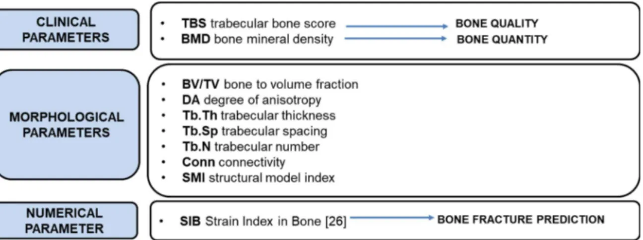
For the clinical assessment of bone two parameters are usually used for determining the bone quality and bone quantity: trabecular bone score (TBS) and bone mineral density (BMD) respectively. BMD and TBS are considered as complementary parameters that can assess bone strength; the former is related to the bone quantity, its resistance to damage and its loading sensitivity while the latter provide an accurate bone quality assessment, and it is affected by the presence of damage. Figure 2.6 shows the microstructural difference between two lumbar vertebrae with similar BMD and different TBS.

8

Despite its primary role in assessing bone strength, BMD only accounts for about 70% of fragility fractures while the remaining 30% could be explained by the impact of other bone quality parameters such as the geometric and material ones, which contribute to fracture resistance independently of bone mineral density [21] [22].

BMD and TBS are measured through the use of DXA, Dual-X Ray Photon Absorptiometry, a system that produces 2D data output using an X-Ray source.

Figure 2.7 Healthy bone on the left and osteoporitic one on the right

Figure 2.6 DXA comparison between an healthy bone on the left and an onsteoporotic one on the right, adapted from [23]

9

The Xray source is mounted beneath the patient and generates a narrow, tightly collimated, fan shaped beam of X-Rays. The energy of X-Ray beams that are passed through bones is absorbed, and what is not absorbed is detected. The denser are the bones, the more energy is absorbed, and less the energy detected. The radiation energy per pixel is detected and converted into a Bone Mineral Density (BMD) while Trabecular Bone Score (TBS) is a textural index that evaluates pixel gray-level variations in the lumbar spine DXA image, providing an indirect but highly correlated evaluation of trabecular microarchitecture [23].

The comparison between a healthy bone and osteoporotic one, Figure 2.7, helps in clarifying how TBS is computed and what information contains.

A healthy trabecular bone has a well-defined structure, dense with thick and compact trabeculae. If this structure is projected onto a plane, the resulting image contains a large number of pixel variations with small amplitudes. On the other hand, an osteoporotic bone has a more porous trabecular tissue with thin trabeculae and projecting this structure onto a plane, the image obtained contains a low number of pixel value variations, but the amplitudes of these variations are high.

A variogram of the trabecular bone projected image is a method that can distinguish between these two kinds of structures, therefore it can provide useful information regarding 3D structure.

2𝛾(ℎ) = 𝐸 𝑍(𝑥 + ℎ) − 𝑍(𝑥) = 1

𝑁(ℎ) 𝑍(𝑥 + ℎ) − 𝑍(𝑥)

( )

In probabilistic notation, the variogram is defined as the sum of the squared grey-level differences between pixels at a specific distance where 2γ(h) is the variogram, x is the vector of spatial coordinates, h is the lag distance, Z(x) is the grey-level function at the coordinate x and N(h) represents the number of pairs separated by lag h.

TBS is calculated as the slope of the log-log transformation of this variogram. A steep variogram slope with a high TBS value is associated with better bone structure, while low TBS values indicate worse bone structure.

10

An elevated TBS appears to represent strong, fracture-resistant microarchitecture, while a low TBS reflects weak, fracture-prone microarchitecture [24].

A recent study [25] has introduced a new parameter that could be used, together with BMD and TBS to improve improve the fracture risk assessment and support the clinical decision to assume specific drugs for metabolic bone diseases. This parameter, SIB (strain index of bone) is one simple DXA-based and FE-models. Bone is simulated as elastic and inhomogeneous material, with stiffness distribution derived from DXA greyscale images of density. The numerical procedure simulates a compressive load on each vertebra to evaluate the local minimum principal strain values. From these values, both the local average and the maximum strains are computed over the cross sections and along the height of the analysed bone region, to provide a parameter, named Strain Index of Bone (SIB), which could be considered as a bone fragility index. Unfortunately, this methodology has some drawbacks, SIB is based on 2D DXA images so it simplifies a 3D problem into a 2D one, losing information on the complexity of bone microarchitecture. SIB is also based on linear elastic models so no damage law is included and the correlation between different clinical, mechanical and morphological parameters are estimated before damage manifestation, i.e. from linear elastic loading, and at the beginning of the damage, which can be identified by the yielding.

2.3

Morphological parameters

To improve the clinical assessment and to quantify the interconnected network of trabeculae there are several structural parameters that become fundamental for the knowledge of bone fragility: morphological parameters.

Micro-CT-based morphological parameters are often used to quantify the structural properties of trabecular bone. Various software tools are available for calculating these parameters [26]. In this thesis the image analysis has been done through the use of the ImageJ software, plug-in BoneJ.

Some of the main structural indexes are enlisted in the following lines:

 Volume Fraction, BV/TV. It measures the bone volume with respect to the total volume

11

 Trabecular Number, Tb.N. trabecular number density of the trabeculae  Trabecular Thickness, Tb.Th., and Trabecular Spacing, Tb.Sp. They

measure the trabecular width and the struts distance respectively

 Degree of anisotropy, DA. It is an adimentional index that defines the geometrical degree of anisotropy; it is ranged from 0 to 1 in which 0 means total isotropy and 1 total anisotropy.

 Connectivity Density, Conn.D. It measures the number of connected structures in a network and it can be computed by dividing the connectivity estimate by the volume of the specimen.

 Structural Model Index, SMI. It gives a general idea of the trabecular bone architecture; in particular plate-like structure tends to 0 while rods-like ones tend to 3 and sphere structures to 4. This index, computed in ImageJ, cannot be used in scientific analysis because of its low accuracy [27]

The Figure 2.8 gives numerical data of Micro-CT studies of Vertebrae in order to have a general idea of the range of values for each parameter. [28]

Many studies investigated which trabecular bone parameter predicts most accurately the mechanical properties of trabecular bone tissue [29]. Most of them stated that bone volume fraction (BV/TV) and fabric anisotropy (DA) are the two main parameters that explain together more than 90% of the variation in trabecular bone tissue elastic properties [30].

12

In particular an interesting study [8] focuses its attention on how mechanical properties of porous structures depend on the volume fraction of the structure and applied strain rates. The elastic modulus, peak stress and energy absorption increased by more than two times when the volume fraction of samples increased from 20% to 40%. The mechanical properties show weak dependency on applied strain rate, only in the post yield regime the effect of strain rate becomes more pronounced.

This thesis focuses its attention on BV/TV and DA indexes, trying to find a reliable correlation between them and the experimental values. They are adimensional parameters that enable to easily compare the real bone values with the 3D polymer printing ones, computed in the post processing image analysis. DA and BV/TV are material independent, highlighting the importance of trabecular bone microstructure in the mechanical behaviour.

All the parameters that have been discussed in Paragraph 2.4 are summarized in Figure 2.9.

13

2.4

Microarchitecture visualization through the Micro-CT

Micro-Computed Tomography, Micro-CT, is an essential tool for studying bone structure and function relations, disease progression, and regeneration in preclinical models and it has facilitated numerous scientific and bioengineering advancements for the development of new tissue engineering strategies over the past 30 years [31] If medical scanners usually have resolutions in the mm range, Micro-CT systems typically achieve resolutions in the 1–100 µm range.

Micro-CT is a non-destructive imaging modality can produce 3D images and 2D maps with voxels approaching 1 μm, giving it superior resolution with respect to other techniques such as ultrasound and magnetic resonance imaging (MRI), even thought, differently from Clinical-CT, it is not suitable to acquire images in vivo [32]. Today, Micro-CT has been used in several studies. For example, in a scaffold optimization study [33], Micro-CT provides comprehensive data on porosity, surface-to-volume ratio, interconnectivity, and anisotropy for non-destructive quantification of microstructural characteristics. Lin and colleagues [34] used Micro-CT to demonstrate the effect of longitudinal macro-porosity and porogen concentration on volume fraction, strut density, and anisotropy in oriented porous scaffolds. Other studies used Micro-CT potential to reconstruct the trabecular structure of bone samples to build a model of the structure in form of a .stl file. These files can be used to 3D-print the models or perform numerical simulation with FEM as it has been done for the samples of this work. Create .stl file from Micro-CT is not immediate but it requires post-processing procedures on image slices and several software are nowadays available, e.g. ImageJ as used in this project.

14

2.5 Finite Element Models

Finite element analysis (FEA) is a useful tool for the analysis of bone biomechanical function. It has been used in bone research for more than 30 years and it has had a substantial impact on the understanding of the complex bone behaviour. It is possible to use FEA for analysis at different hierarchical level, as shown in Figure 2.10, each analysis provides further information about the relationship between bone structure and its peculiar mechanical behaviour.

[35]

FEA has been used to perform simulations on trabecular bone structures in many studies, for example to perform a non-invasive assessment of in-vivo bone using a model from clinical CT [36], to predict the vertebral compressive strength [37] or to predict apparent stress and strain at failure and how the damage is concentrated [38].

It is possible to define two main approaches that have been generally considered in FEA models. The first approach is based on cellular solids theories while the second one combines micro-FE with high-resolution images. The latter is the one used for this thesis.

15

Cellular solids approach aims to simplify the complexity of the trabecular network without losing its specific mechanical aspects and this is possible by mapping only certain aspects of the cancellous bone into simplified 2D or 3D lattice models. The microstructure of a cellular solids model is often composed of a collection of elements that can be regularly arranged in space (eg, periodic honeycombs). They are idealized representations of the trabecular architecture that enables to evaluate how the variation of a specific architectural parameters can impact in the mechanical behaviour of bone, investigating the effect of different degrees of disorder on apparent stiffness or strenght [35].

Luxner and colleagues [39] showed that introducing some disorder into a regular cellular lattice had a positive mechanical outcome since it reduced the tendency of deformation localization (Figure 2.11) and it decreased the strong anisotropy of the cubic lattice. By applying these results for trabecular bone structures, it can be assumed that some disorder in the arrangement of trabeculae might be beneficial to prevent or retard catastrophic failure.

Concerning the other approach, in micro-FE studies, cancellous tissue is normally considered homogeneous and isotropic and the same Young’s modulus is given to each element. This assumption is accurate enough for predicting the apparent elastic properties of trabecular bone specimen, as reported by several authors [40] [41]. By comparing experimental versus micro-FE models is even possible to derive an apparent or effective modulus for the trabecular tissue.

Literature reports different values for Young’s modulus, in the range 5–18 GPa and this wide range reflects natural biological variability (eg, anatomical site, age) as well as differences in the experimental techniques, specimen size and element size [42].

16

Whereas for quantifying the elastic properties at the apparent level an effective tissue modulus works well, when considering the mechanical behaviour of individual trabeculae this assumption might not be too accurate. Trabecular tissue indeed is heterogeneous and anisotropic as a result of bone remodeling and mineralization. Improvement in the prediction of the mechanical behaviour (can be obtained by employing more complex material laws. Chevalier et al. [43] used a calibration method to derive local bone volume fraction (BV/TV) from BMD values and a fabric-based model was adapted to convert local voxel volume fractions into elastic values. With this novel procedure, each element of the FE model carries information on local elasticity as well as on the anisotropy of the trabecular network.

The validity of this procedure is still controversial because of two issues. First, it is not clear how to rightly convert the gray levels of Micro-CT image into proper mineral contents and even if calibration steps are implemented, the voxel values of micro-CT images are influenced by image artifacts. Secondly, there is still uncertaninty in the relationship between local mineral content and local elastic properties [44] In conclusion, micro-FE modeling provides excellent estimates of trabecular bone mechanical properties when considered at a scale where it behaves as a continuum. Whether it currently provides the same accuracy at the level of single trabeculae still remains to be established. For that purpose, more studies which combine micro-FE with accurate experimental measures of local mineral content and local tissue moduli are needed. It appears that the heterogeneous material distributions as seen in trabeculae could have a strong effect on the mechanism of deformation and failure especially for those trabeculae subjected to large deformations [35]

FEA solutions are approximation of the reality and it is impossible to deal with this kind of analysis without considering concepts like accuracy and validity. The accuracy of a FE model, quantifying the difference between the model output and the real solution of the problem. In order to estimate the accuracy of the model it is possible to run a convergence test: the size of the element is gradually decreased and a new solution is obtained and compared with the old one until the variation of the simulation outcome is negligible.

17

From a mathematical point of view, if the element size approaches zero, the numerical solution will converge to the correct solution.

The model validity is another fundamental issue that defines the extent of the results of the model, highlighting where the model can predict the behaviour of the investigated real system. Set the correct mesh size and define the best boundaries conditions are the most critical and challenging steps in the FE model development as it will be discussed in Chapter 3 [45] [30] for the computation of the elastic modulus in a human vertebra model.

Figure 2.12 Femoral head specimen with different voxel resolution (84 µm on the left and 168 µm on the right) and different mesh geometry (hexahedron mesh at the top and tetrahedron one at the bottom)

18

As an example, the Figure 2.12 shows four different models of a femoral head specimen created at a voxel resolution of 84 µm (left) and 168 µm (right) using either the hexahedron meshing (top) or the tetrahedron meshing approach (bottom) Once validated, finite element model is a powerful tool that allows one to simulate the mechanical behaviour of a specific structure under certain boundary and loading conditions without having to perform an experimental test for each changing condition [46]. To reduce computational cost, some studies start from a bigger global model, then they select a sub-region of interest and make a more detailed simulation on this [47]. In this thesis, the same approach was used in order to obtain more information of the models that are not possible to get from the global model due to its limitation in the mesh size.

2.6 Additive manufacturing for bone studies

Nowadays, Additive Manufacturing (AM) is an innovative technique that finds multiple applications in bone tissue engineering. It has been used for to repair and regenerate bone but also to provide knowledges of bone biology and structure. In the medical field, this technology has been developed for the creation of customised human hard tissue in a cost-effective way. AM is used for surgical applications: anatomical models aid pre-surgical planning and education.

19

Tissue engineering is used to regenerate and replace tissue or organs damaged by injury, disease or any other congenital anomalies. Additive manufacturing combines together tissue engineering, material science and regenerative medicine to repair bone. In particular, damaged tissue and organs are repaired with scaffolds that have been created through 3D printing systems (e.g Figure 2.13).

In contrast to macroscale biomodels of large bones those at the microscale represent very small structures: trabecular bone is a typical example of such microscopic structure. For these fine models, the resolution of conventional CT is not sufficient and high-resolution technique such as Micro-CT scanning is required to obtain all information necessary to generate accurate models. The acquired images can be reconstructed, segmented and modified according to the requirement in post-processing software and it is finally possible to generate a 3D CAD model. This one can be exported to a 3D printer and several replicas of the original sample can be reproduced.

The complexity of the geometry and problems related to the fact that every trabecular bone is unique, are fortunately overcome with the recent advancement in 3D printing technology.

Depending on the process used to fabricate a physical model, when the resolution of the process is not sufficient, enlargement of the model is advantageous. This is especially valid when mechanical tests will be carried out on the model, e.g compression tests. The aim of these tests is the determination of relationship between changes in trabecular microarchitecture and changes in overall elastic stiffness and failure strength.

In such situations, enlarging the model would yield greater geometrical accuracy and hence more reliable results. It would also facilitate optical inspection of both structure and deformation patterns. In this thesis the original bone sample have been enlarged 3 times in order to enhance the morphological structures that are at the center of the analysis.3D printing represents a wise solution that can solve the problem of having a unique structure infact it is possible to test the same structure under various mechanical loading conditions.

20

Literature reports many examples of 3D printing techniques employed for reproducing the trabecular structure itself. There are studies that take advantage of this manufacturing approach, for example, to quantify the effect of osteoporosis on the mechanical properties of the same trabecular structure, by 3D printing the healthy trabecular bone model and the same model after bone resorption has been simulated.Another study [8], instead, aims to quantify the effect of osteoporosis on the mechanical properties of the same trabecular structure simply by tuning the BV/TV of the starting sample as you could see in Figure 2.14.

Unfortunately, 3D printing has some drawbacks. A past study has shown how different process parameters affect the final result, pointing out the importance of carefull planning, controlling steps and detailed reporting of the used parameters. It highilights the significant variability of the mechanical properties of different samples from a specific bone scaffold ordered from the same producer at different times [48] It focuses its attention on different parameters, affecting the production the sample: the time gaps between completion of the printing job, removal of the support material, and mechanical testing, the water solution temperature, the saturation level at which the water bath is refreshed, and as a result the amount of residual support material within the sample considerably affect the mechanical properties of the samples.

Figure 2.14 Reconstructed 3D model of the interested TB zone (30% VF) and modified models for volume fractions (20% and 40%) with the corresponding top view. [8]

21

3D printing is not just a useful tool for the study of bone structure but it is widely used in the development of meta-materials, in particular for building materials with a bone-inspired structure, such as high-porosity micro-architectured materials, to obtain enhanced fatigue properties [16], or as hierarchical structures to emulate the toughness amplification of cortical bone [49].

Understanding the behaviour of bone tissue at micro-scale could lead towards interesting development, not only in medical field but also in several other applications that looks at bone structure as a source of inspiration for its peculiar features.

2.8 General objectives

This thesis is a preliminary study that lays the foundation for a wider project whose aims are:

 Study the morphology influence on bone mechanical resistance in compression. The use of 3DP replica helps to overcome the material influence, focusing only on trabecular network

 Comprehension of the correlation between the experimental results from the mechanical tests and the morphological parameters

 Generation of a global finite element model that resembles the mechanical behaviour in compression of the 3D printed samples. Once validated, the FE model can give complementary information (e.g stress-strain distribution), becoming an useful tool for the creation of new prosthetis implant or for optimization study.

 Definition of the weakest zone in the sample at trabecular level in terms of mechanical resistance, pointing out the architecture of this specif area. Understand the type of failure mechanism that had occurred and the causes of damage.

22

MATERIALS AND METHODS

3.1

EXPERIMENTAL SECTION

The main topics of this experimental section are:

 Sample preparation from the origin of the structure to the 3D-printing and the post-processing

 Micro-CT from the scanning procedure to the processing of the digital images

 Compression test from the definition of the test procedures to the analysis of the results

In Figure 3.1 a scheme of this section is represented.

23

3.1.1 Original porcine samples

The six samples used in this work were printed to replicate the structure of porcine vertebrae trabecular bone coming from the previous work headed by Mirzaali, Libonati et al. [50], [23]. The porcine trabecular specimens in that study were extracted from the body of the lumbar vertebrae of six different animals of one and a half years old. The cutting procedure is described in Davide Ferrario’s thesis [23]: “Samples were drilled using a drilling device (WÜRTH®) along with the anatomical direction of the vertebral column. The coring device had the inside diameter of 16 mm and length of 40 mm. Subsequently, the samples were transferred to a lathing machine (OPTIMUM®) to reduce them to cylinders with the diameter of about 13.85 mm and height of 30 mm. During the drilling and milling, specimens were kept wet with water. […] To have perfectly parallel surfaces, both ends of bone specimens were smoothened using a circular blade saw (abrasive cutting instrument HITECH EUROPE)”. The .stl files used for 3D printing were generated from images adquired by Micro-CT (the details about the machine will be provided in the paragraph 2.1.3 as it is the same of the current work) The spatial resolution used was of 25.6 μm and 26.3 μm and the parameters of the scanning were fixed at 60 kV and 150 μA. Specimens were submerged in saline solution during the scanning to simulate the physiological conditions of the body.

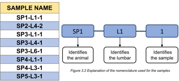
The samples in this thesis work will be identified as the corresponding porcine bone samples and are reported in Table 3.1 and the nomenclature is explained in Figure 3.2.

24

3.1.2 3D printing

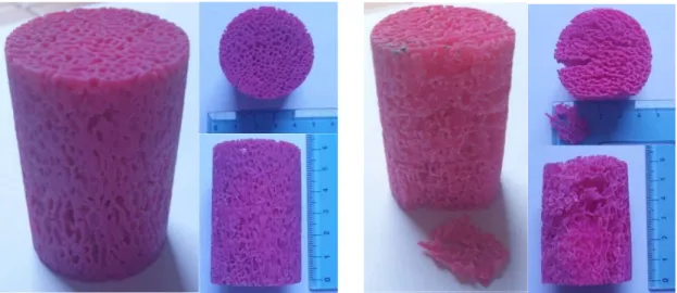
With respect to the original porcine bone specimen, the dimensions were scaled 3 times larger and an external annulus was removed in the creation of the .stl models. The samples were printed in an acrylic‐based photopolymer called VeroMagenta (RGD851), at Massachusset Insistute of Technology. Mechanical properties of this material are reported in Table 3.2. A cleaning step was necessary in order to remove the wax-like support material (SUP706); samples were cleaned first by Waterjet, then submerged in an alkaline solution of water with the addition of 2% NaOH (CAS 1310-73-2) ad 1% Na2SiO3 (CAS 6834-92-0), and placed into a home-built cleaning station. Nevertheless, it is not possible to exclude its presence in some closed cavities. Two samples are shown in Figure 3.3. [51]

SAMPLE NAME

SP1-L1-1

SP2-L4-2

SP3-L1-1

SP3-L4-1

SP3-L6-1

SP4-L1-1

SP4-L3-1

SP5-L3-1

Density [Kg/m3] Stiffness [MPa] Strength [MPa] Elongation at

breakage [%] Toughness [MJ/m3_] 1170 2187 ± 404 46.41 ± 3.23 9.8 ± 2.0 3.54 ± 0.75

SP1

L1

1

Figure 3.2 Explanation of the nomenclature used for the samples Table 3.1 Names of the 3D-printed

samples considered in this thesis work

25

Samples dimensions and weight have been measured and the volume fraction BV/TV has been calculated. Equation 3.1 shows the calculation of bone volume, where m is the weight of the sample and ρ is the density of VeroMagenta. Equation 3.2 shows the calculation of total volume of the sample, that is the volume of the virtual cylinder that envelopes the sample, where d is the diameter of the sample and h its height. The bone volume fraction calculation is reported in Equation 3.3.

𝐵𝑉 =𝑚 𝜌 𝑇𝑉 =𝑑 𝜋 4 ℎ 𝐵𝑉 𝑇𝑉 = 4𝑚 𝜌ℎ𝑑 𝜋

Figure 3.3 Left: SP1-L1-1 3D-printed sample. Right: SP3-L6-1 3D-printed sample, already damaged

Equation 3.1 Calculation of bone volume of the sample

Equation 3.2 Calculation of total volume of the sample

26

The dimensions and weight measured are reported in Table 3.3 together with calculated BV/TV

Table 3.3 Samples measures and calculated BV/TV

3.1.3 Scanning Procedure: Micro-CT

Micro-Computed Tomography is an imaging technique based on the absorption of x-ray radiation at a specific wavelength characteristic of the material. Its equipment is made up of an x-ray tube, radiation filter and collimator (which focuses the beam geometry), specimen stand, and a detector. X-ray radiation is emitted by a source and pass through the sample, finally projecting the image on the detector. The sample is then rotated by a fraction of a degree and another projection image is taken at the new position. This procedure is repeated up to a complete rotation. A computer software re-elaborates the projected images and the internal structure of the object is reconstructed through a series of slices that correspond to the cross sections of the sample as it is explained in Figure 3.4. [52]

SAMPLE NAME Average Height _[mm] Average diameter _[mm] Weight [g] BV/TV [weighted]

SP1-L1-1

SP2-L4-2

SP3-L1-1

SP3-L4-1

SP3-L6-1

SP4-L1-1

SP4-L3-1

SP5-L3-1

27 As an x-ray passes through tissue, the intensity of the incident x-ray beam decrease according to the Equation 3.4, where I0 is the intensity of the incident beam, x is the

distance from the source, Ix is the intensity of the beam at distance x from the

source, and μ is the linear attenuation coefficient. 𝐼 = 𝐼 𝑒

The attenuation therefore depends on both the sample material and source energy and can be used to quantify the density of the tissues being imaged when the reduced intensity beams are collected by a detector array. Beam energy choice is relevant and some studies have pointed out the impact of this parameters on image quality [53].

Micro-CT images of trabecular specimens were collected using an x-view scanning equipment (North Star Imaging 3D X-ray CT X25 shown in Figure 3.5) that has a

Figure 3.4 Micro-CT acquisition process and output adapted from [52]

28

maximum spatial resolution of 5 μm. The parameters of the scanning were fixed at 56 kV and 125 μA, with a spatial resolution of 18.4 μm. In the Appendix A there are the files with the complete list of used parameters. Two batches of four specimens each were placed in the CT equipment. To distinguish the samples, three metallic wires fixed with some clay were added into the chamber.

The dedicated software efx® _{CT software has performed image reconstruction,}

giving as output three sets of 2D slices of the samples, one set for each coordinate.

3.1.4 Image analysis

The open source sofware ImageJ Fiji was used for the post processing and analysis of the sample. The set of slices were elaborated to obtain binary images and .stl files for the computational part. The steps used to obtain the final result are the following:

1. Isolate the samples: the two batches are constituted by 4 samples each, with the cut tool each sample is separated

2. Rotate the samples: due to the presence of the clay, the samples were standing on an angled support

3. Set the correct scale selecting a known distance, the measured diameter of each sample

4. Enhance contrast to have a better distinction of the structure with respect to the background

5. Apply a proper filter, in particular Gaussian Blur filter was chosen. 6. Binarize the images using Otsu as method with dark background.

29

7. Create an .stl model from the calculation of the isosurface of the set of slices. 8. Measure volume fraction and anisotropy of the sample.

In Figure 3.6 the main steps to obtain binarized slices are represented (rotation and setting scale are placed between step 2 and 3).

Gaussian Blur filter

The aim of this step is to reduce as much as possible the noise without losing too much information by doing a weighted average of the pixels in their neighborhood. Gaussian Blur is one of the most used filter types for the purpose [54].

As Micro-CT is important for the adquisition of image slices, post processing image is a challenging step that plays a central role. Noise can be present and it could be related to several sources, affecting image quality. It is important to filter images before segmentation and analysis, without losing data nor changing images. Gaussian filter is largely used, during image post processing, for noise removal. Gaussian filter is a type of image-blurring filter, that uses a Gaussian function for computing the transformation to be applied to each pixel in the image.

30

A convolution matrix is applied to the original image using values from the distribution, as it is described in Figure 3.7. When applied in two dimensions, this formula produces a surface whose contours are concentric circles with a Gaussian distribution from the center point. Each pixel's new value is set to a weighted average of that pixel's neighborhood. Central pixel has a higher weighting than those on the periphery that have smaller weights as their distance to the original pixel increases. At the edge of the maske, coefficients must be close to 0.

The neighborhood for this filter is set by using the sigma and support value. The first is the standard deviation of neighborhood while the second considers the size of the neighborhood pixels. A larger sigma value, σ, produces wider peak in the Gaussian distribution, that is translated in having a greater blurring effect on the image. This filter gives and effective smoothing effect on images and it helps in noise removal but it is not particularly effective at removing salt and pepper noise defects [55]. Gaussian filter has been used in this thesis in order to improve image quality after Micro-CT; the choice of the right sigma value has been a critical aspect as it will be better explained in Chapter 4.

Otsu Binarization

This step is fundamental to determine the contour of the structure. A binary image is produced by quantization of the image gray levels to two values, usually 0 and 1. Binarization consists in two steps, the first is the determination of a gray threshold according to some objective criteria and the second is assigning each pixel to the background, in case its intensity is lower than the threshold or otherwise to the foreground. Otsu’s thresholding technique is a method based on searching for the

31

threshold that minimizes the intra-class variance, defined as a weighted sum of variances of the background and foreground classes. [56] An example of how this threshold appears is in Figure 3.8, where it is possible to see how the red line splits the spectrum in two parts of the same area.

Otsu binarization is not the only thresholding technique used in this thesis work, even though it was the starting point.

Manual Thresholding

This method is based on tuning the threshold of a filtered stack of slice to choose a value that will be able to better fit the sample. It can be coupled with a measure of the samples real BV/TV, for example using the Archimede’s principle [57], or it can be use to simulate the effects of osteoporosis on a trabecular structure [30]. In the present case, the threshold was tuned to reproduce the BV/TV of the value found by weighting SP1-L1-1 sample.

This technique can be really useful in the case that the trabecular structure is well reproduced by micro-CT, but it cannot help the cases where thin trabeculae are lost in the scanning process, as it would only thicken the already present ones, modifying the actual structure of the model.

Figure 3.8 Form SP1-L1-1-1 slices on ImageJ. Left: image with applied Gaussian filter (σ=2); Centre: binarized image with Otsu method; Right: Otsu threshold in red on the spectrum of the first image

32

Isosurface generation

BoneJ plugin in Fiji has been used to build the isosurface of the set of images. This algorithm uses the marching cubes method [58] for building the triangular mesh. This algorithm uses a divide-and-conquer approach to locate the surface in a logical cube created from eight pixels, four each from two adjacent slices, as it is shown in Figure 3.9 on the left. As it determines how the surface intersects the cube, it moves to the following cube. According to the position of the surface with respect to each vertex of the cube, a 1 will be assigned if the surface is below the vertex and a 0 otherwise; so there are 28_{=256 different ways a surface can intersept the cube, in}

Figure 3.9 there are some examples on the right. The position of the polygon verteces along the cube's edge is found by linearly interpolating the two scalar values that are connected by that edge.

This isosurface algorithm allows for a resampling of the digital volume: a low resampling leads to a very accurate but heavy mesh, and a high resampling leads to a mesh with less triangles and so low accuracy. As this triangular mesh will not the one used in FEM, the default value of resampling 6 was used. An example of the result is shown in Figure 3.10.

Figure 3.9: Marching cube algorithm. Left: the identification of a single cube between two consecutive slices; right: examples of how the different intersections between cube and surface are numerated.

33

BV/TV and DA calculation

BoneJ plugin was also used to calculate the volume fraction and the anisotropy of the samples. Using the oval tool, a circular area containing the cross-section of the sample was selected. The volume fraction was calculated using the voxel algorithm and the anisotropy was calculated selecting the Auto-Mode option.

A MatLab script (Appendix D) was also used to calculate the BV/TV slice-by-slice, in order to see the trend along the height of the sample.

It has to be noticed that, due to rotation and the presence of slices in which the clay and the wires ruin the images, some slices were removed from the top and the bottom of the sample. So the binarized stacks of slices and consequently the .stl models obtained are shorter than the corresponding sample. In Table 3.4 the dimensions of the final stacks of slices are reported.