Universit´
a di Pisa
Facolt´a di Scienze Matematiche Fisiche e Naturali
Corso di Laurea Specialistica in Scienze Fisiche
Anno Accademico 2006-2007 Tesi di Laurea Specialistica
On Non-Gaussianity of the
Cosmological Perturbation
Candidato: Giovanni Petri Relatore: Dr. Antonio Riotto
Contents
1 Introduction 4
2 Big Bang and Inflation: an overview 13
2.1 Basics of the Big-Bang Model . . . 13
2.1.1 Friedmann Equations . . . 14
2.1.2 Early Universe Formalisms . . . 16
2.1.3 The Early Radiation-dominated Universe . . . 18
2.2 The Problems of Big Bang Theory . . . 20
2.2.1 The Flatness Problem . . . 20
2.2.2 The Entropy Problem . . . 21
2.2.3 The Horizon Problem . . . 22
2.3 The Inflationary Paradigm . . . 24
2.3.1 Inflation and Cosmological Perturbations . . . 29
2.3.2 Quantum Fluctuations of a Generic Scalar Field during a de Sitter Stage . . . 32
3 The Curvature Perturbation ζ 38 3.1 ∆N Formalism . . . 38
3.1.1 Separate Universes and Geometry . . . 38
3.1.2 Slicings . . . 43
3.2 Non-adiabatic Perturbations and Evolution of ζ . . . 46
3.2.1 Multiple Adiabatic Fluids . . . 48
4 Non-Gaussianity 50 4.1 Scenarios . . . 50
4.1.2 The Curvaton Scenario . . . 53
4.1.3 Experimental Limits on Non-Gaussianity Parameters . 55 4.2 N -point Functions and Spectra . . . 56
5 CTP Formalism 64 5.1 Basic Formalism . . . 66
5.2 Green’s Functions . . . 67
5.3 Feynman Rules . . . 70
6 Loops and Correlation Functions 73 6.1 Two-Point Functions . . . 74
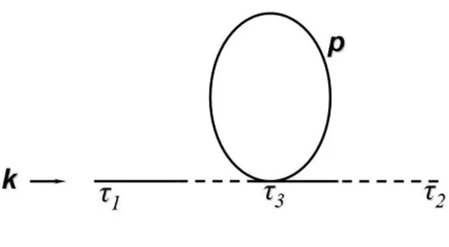
6.1.1 First Order Diagrams . . . 74
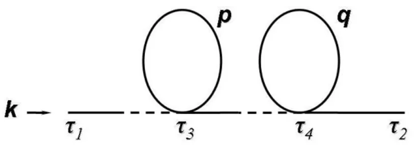
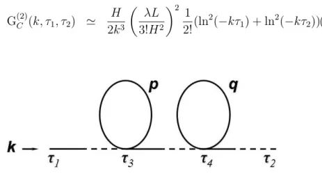
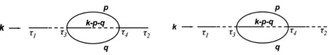
6.1.2 Second Order Diagrams . . . 77
6.1.3 Higher Order Diagrams . . . 85
6.2 Four Point Functions . . . 94
6.3 Diagrams Selection and O(N ) symmetry . . . 100
Chapter 1
Introduction
Since its accidental discovery by Penzias and Wilkinson in 1965, the Cosmo-logical Microwave Background radiation (CMB) has been one of the funda-mental observational pillars of the Big Bang cosmology, together with the Hubble diagram and the prediction of light element abundances. It has pitched the balance of opinion from the Steady State cosmology, proposed by Fred Hoyle, Thomas Gold, Hermann Bondi and others (see for example [1]) to the dynamical Big Bang view. The first measurements showed with good approximation a blackbody spectrum that well suited the idea of a hot, dense, opaque ball of expanding gas. During its first moments, the Universe was thought to be in full thermal equilibrium, with photons being continu-ally emitted and absorbed, giving the radiation a blackbody spectrum. As the Universe expanded, it cooled to a temperature at which photons could no longer be created or destroyed. The temperature was still high enough for electrons and nuclei to remain unbound, however, and photons were ef-ficiently scattered, keeping the early Universe opaque. The characteristic transparency of the present Universe came later, when the temperature fell to a few thousand Kelvin, so that electrons and nuclei began to recombine. Since photons scatter infrequently from neutral atoms, radiation decoupled from matter when nearly all the electrons had recombined, at the epoch of last scattering (z ≃ 1100), about 300,000 years after the Big Bang. These free streaming photons were subsequently redshifted by the expansion, which preserved the form of the spectrum but caused its temperature to fall,
mean-ing that the CMB photons now fall into the microwave region. The radiation is thought to be observable at every point in the Universe and comes from all directions with (almost) the same intensity. It was exactly the observed isotropy of the CMB to open the way to the inflationary paradigm. The Hub-ble horizon HLS−1 at the last scattering was much smaller than the horizon
we would obtain tracing back the present one (H0−1). Looking at angular
scales on the sky corresponding to HLS−1 we find that all those regions look
like they were in thermal equilibrium at the last scattering. Yet, if we assume a radiation or matter dominated Universe and we trace back those regions we find that they were not even in causal contact. So the high isotropy of the CMB prompted the first reflections about how non causally connected regions could share the same properties. The Big Bang Universe needed a way to expand faster, much faster. Inflation, first proposed by Guth in 1981
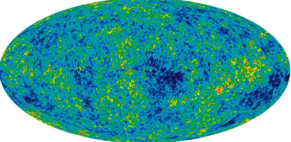
Figure 1.1: A graphical representation of the expansion of the Universe with the inflationary epoch represented as the dramatic expansion the left [WMAP press release, 2006]
[2], was born.
In the first formulation Inflation involved a brief period of rapid exponential expansion of the scale factor a, driven by the energy density of a scalar field, the inflaton, trapped in a false minimum of its potential. In this scenario, small localized regions would tunnel to the true vacuum and start growing. For the Universe to move as a whole to the true vacuum though these bub-bles would need to coalesce. Careful calculations showed that they would not [3, 4]. To avoid the problem Linde, Albrecht and Steinard in 1982 [5, 6] made use of a scalar field slowly rolling to its minimum. The energy density of such a field is thought to be very close to constant and so it comes quickly to dominate the energy balance and thus drive Inflation.
In 1992 the Cosmological Background Explorer (COBE) detected for the first time CMB temperature anisotropies [7, 8] at a level of 1 part in 105.
These anisotropies are the sign of perturbations at the last scattering sur-face. Inflation again provided an elegant explanation: microscopic quantum fluctuations of the inflaton field were magnified to cosmological scales dur-ing the inflationary era, generatdur-ing cosmological curvature perturbations and thus creating matter perturbations, the primordial seeds for the structures that we observe today. As fluctuations wavelenghts were stretched by the ex-ponential expansion, they eventually became larger than the horizon, which grew slower than a. This phenomenon is referred to as horizon exit: while outside the horizon the fluctuations freeze [5, 9], their amplitude remain-ing constant since they are larger than the scale over which causal physics can operate. After the end of Inflation, the frozen fluctuations gradually reentered the horizon becoming thus observable. Thus, the larger scale per-turbations that we observe now were the ones who exited the horizon earlier during Inflation and therefore they are also the ones less likely to have been modificated by causal under–horizon interactions.
The last confirmation of the inflationary paradigm has been recently pro-vided by the data of the Wilkinson Microwave Anisotropy Probe (WMAP) mission [10]. The WMAP collaboration has produced a full–sky map of the angular variations of the CMB and a plot of the temperature anisotropies, with unprecedented accuracy (respectively fig. 1.3 and 1.2). WMAP data confirm the inflationary mechanism as responsible for the generation of
cur-vature (adiabatic) superhorizon fluctuations [11].
Figure 1.2: The power spectrum of the cosmic microwave background ra-diation temperature anisotropy in terms of the angular scale (or multipole moment).The correlations observed in the gray–shaded area on the left side of the first peak are the signature of the inflationary expansion. The data shown come from the WMAP (2006).
Since the primordial cosmological perturbations are tiny, the generation and evolution of fluctuations during Inflation havef been studied within linear perturbation theory. Within this approach, the primordial density pertur-bation is Gaussian; in other words, its Fourier components are uncorrelated and have random phases. Despite the simplicity of the inflationary paradigm, the mechanism by which cosmological adiabatic perturbations are generated is not yet established. In the standard slow–roll scenario associated to one– single field models of Inflation, the observed density perturbations are due to fluctuations of the inflaton field itself when it slowly rolls down along its potential. When Inflation ends, the inflaton φ oscillates about the minimum
Figure 1.3: The detailed, all-sky picture of the infant Universe from three years of WMAP data. The image reveals 13.7 billion year old temperature fluctuations (shown as color differences) that correspond to the seeds that grew to become the galaxies [WMAP press release].
of its potential V (φ) and decays, thereby reheating the Universe. As a result of the fluctuations each region of the Universe goes through the same his-tory but at slightly different times. The final temperature anisotropies are caused by Inflation lasting for different amounts of time in different regions of the Universe leading to adiabatic perturbations. Under this hypothesis, the WMAP dataset already allows to extract the parameters relevant for distinguishing among single–field Inflation models [11, 12].
However, what if the curvature perturbation is generated through the quan-tum fluctuations of a scalar field other than the inflaton? Consider, for instance, the curvaton scenario, where the final curvature perturbations are produced from an initial perturbation associated with the quantum fluctua-tions of the curvaton, a light scalar field, whose energy density is negligible during Inflation and curvaton isocurvature perturbations are transformed into adiabatic ones when the curvaton decays into radiation much after the end of Inflation. It liberates the inflaton from the duty of generating the cos-mological curvature perturbation and therefore avoid slow–roll conditions. Their basic assumption is that the initial curvature perturbation due to the
inflaton field is negligible. Other mechanisms for the generation of cosmolog-ical perturbations have been proposed. A few examples are the inhomoge-neous reheating scenario [13, 14, 15, 16], the ghost inflationary scenario [17] and the D–cceleration scenario [18].
So how can we discriminate among them? Different models provide dif-ferent constraints on gravitational waves produced during Inflation, for ex-ample in the curvaton scenario the inflaton potential has to be small enough so that its contribution to the primordial curvature perturbation in the ob-served CMB anisotropy is negligible. Therefore the curvaton mechanisms would produce gravitational waves with an amplitude too small to be de-tectable [19]. A future detection would then favor slow-roll models while a failed detection would not give any information about the generating mech-anisms of perturbations. Another powerful tool to constrain inflationary models is the spectral index nζ calculated from the spectrum of comoving
curvature perturbations: slow–roll models for example predict |nζ− 1| ≪ 1
[20, 21]. Remarkably, the eventual accuracy ∆nζ ∼ 0.01 offered by the
fu-ture Planck satellite [22] is just what one might have specified in order to distinguish between various slow–roll models of Inflation. If cosmological perturbations are due to the inflaton field, then in ten or fifteen years there may be a consensus about the form of the inflationary potential, and at a deeper level we may have learned something valuable about the nature of the fundamental interactions beyond the Standard Model. However, we cannot exclude the possibility that there are other mechanisms for the creation of the cosmological perturbations, which generically predict a value of nRvery close to unity with a negligible scale dependence. Then, it implies that a precise measurement of the spectral index will not allow us to efficiently discrimi-nate among different scenarios. We should then turn to a third observable which will prove fundamental in providing information about the mechanism chosen by Nature to produce the structures we see today. It is the deviation from a pure Gaussian statistics, i.e., the presence of higher–order connected correlation functions of CMB anisotropies. The angular n–point correlation function for temperature anisotropies
¿ δT T (ˆn1) δT T (ˆn2) . . . δT T (ˆnn) À , (1.1)
is a simple statistic characterizing a clustering pattern of temperature fluctu-ations on the sky, δTT (ˆn), where the bracket denotes the ensemble average. If the fluctuation is Gaussian, then the two–point correlation function specifies all the statistical properties of δTT (ˆn), for the two–point correlation func-tion is the only parameter in a Gaussian distribufunc-tion. If it is not Gaussian, then we need higher–order correlation functions to determine the statisti-cal properties: a non–vanishing connected three– or four–point correlation function of scalar perturbations, or their Fourier transform, the bispectrum and trispectrum, are indicators of a non–Gaussian feature in the cosmolog-ical perturbations. The importance of the bi– and trispectrum comes from the fact that they represent the lowest order statistics able to distinguish non–Gaussian from Gaussian perturbations. Thus an accurate calculation of the primordial spectra of cosmological perturbations has become an ex-tremely important issue, as a number of present and future experiments, such as WMAP and Planck, will allow to constrain or detect non–Gaussianity of CMB anisotropy with high precision.
With the coming measurements and the possibility of non Gaussian fields, it becomes important to know how loop corrections to the scalar field influ-ence the correlation functions and whether they must be accounted for in evaluating the non Gaussianity of the curvature perturbation. A number of papers addressed this problem using toy model potential of the form φn
(usu-allu n = 3, 4) and showed that in these theories the first order corrections in perturbation theory produce a logarithmic divergence in the correlation func-tions evaluated at late times during Inflation [23, 24, 25, 26, 27, 28, 29, 30], making the correlations useless for the prediction of non Gaussianity. Yet, none of those papers investigated whether that divergence and the ones aris-ing at higher orders could be cured by means of resummations.
The goal of this thesis is then to investigate whether the resummation is possible. We will start with the free scalar field propagators in a Friedmann Robertson Walker Universe during a de Sitter stage and use them to build the higher order loop corrections for a λφ4 theory. We will then try to resum
a different diagram classes in order to see whether the divergences are reab-sorbed and whether we find evidence that the full theory is not divergent in the late time limit. We will then present an argument to justify our choice
to neglect a large number of diagrams and to focus only on a small selection. Finally we will use the resummed 2–point correlation functions to calculate the 4–point correlation function and the observation of its behaviour for late times will give us an estimate of the non Gaussianity produced by the self– interacting scalar field.
In the next chapters we will slowly build up all the tools needed for this calculation. The thesis is structured as follows:
• Chapter 2 contains a more detailed review of the Big Bang cosmology and of the problems that led to the inflationary paradigm. We intro-duce also the theory of quantum fluctuations for a generic scalar field evolving in a fixed de Sitter background.
• Chapter 3 is about the curvature perturbation ζ that we already men-tioned often. Section 3.21 utilizes the δN formalism to show how ζ is conserved superhorizon for adiabatic perturbations. Section 3.2 on the contrary briefly explains how can ζ evolve, also in case of adiabatic fluids.
• Chapter 4 is devoted to the non Gaussianity of perturbations. Build-ing on the previous chapter, we show explicitly how the level of non Gaussianity can be parametrized in the two case of the inflaton and curvaton scenarios. Then in section 4.2 we put forth the formalism needed to calculate the 3– and 4–point ζ correlation functions and how it relates to the φ correlation functions.
• Chapter 5 introduces the Closed Path Time formalism. We will have to calculate expectation values of correlation functions on vacuum states, but during Inflation it is difficult to define past and future asymptotic states and thus the conventional in–out formalism fails. Therefore a different formalism is needed. In particular in section 5.3 we calculate the Feynman rules of the chosen self-interacting theory.
• Chapter 6 contains the actual calculations of higher order Feynman di-agrams for the self–interacting scalar field. In section 6.1 we calculate the corrections to the two–point propagators and search for a resum-mation. Then, in section 6.2 we use the results to calculate the 4–point
correlation function and discuss its meaning, while in section 6.3 we justify the choice of neglecting certain diagrams.
Chapter 2
Big Bang and Inflation: an
overview
2.1
Basics of the Big-Bang Model
The standard cosmology is based upon the maximally spatially symmetric Friedmann-Robertson-Walker (FRW) line element
ds2 =−dt2+ a(t)2 · dr2 1− kr2 + r 2(dθ2 + sin2θ dφ2) ¸ ; (2.1) where a(t) is the cosmic-scale factor, Rcurv ≡ a(t)|k|−1/2 is the curvature
radius, and k = −1, 0, 1 is the curvature signature. All three models are without boundary: the positively curved model is finite and “curves” back on itself; the negatively curved and flat models are infinite in extent. The Robertson-Walker metric embodies the observed isotropy and homogeneity of the Universe. It is interesting to note that this form of the line element was originally introduced for sake of mathematical simplicity; we now know that it is well justified at early times or today on large scales (≫ 10 Mpc), at least within our visible patch.
The coordinates, r, θ, and φ, are referred to as comoving coordinates: A particle at rest in these coordinates remains at rest, i.e., constant r, θ, and φ. A freely moving particle eventually comes to rest these coordinates, as its momentum is red shifted by the expansion, p ∝ a−1. Motion with respect
velocity. Physical separations between freely moving particles are simply a(t) times the coordinate separation. The momenta of freely propagating particles decrease, or “red shift,” as a(t)−1, and thus the wavelength of a photon stretches as a(t), which is the origin of the cosmological red shift.
2.1.1
Friedmann Equations
The evolution of the scale factor a(t) is governed by Einstein equations Rµν−
1
2R gµν ≡ Gµν = 8πG Tµν (2.2) where Rµν (µ, ν = 0,· · · 3) is the Riemann tensor and R is the Ricci scalar
constructed via the metric (2.1) [31] and Tµν is the energy-momentum tensor.
Under the hypothesis of homogeneity and isotropy, we can always write the energy-momentum tensor under the form Tµν = diag (ρ, P, P, P ) where ρ is
the energy density of the system and P its pressure. They are functions of time. The evolution of the cosmic-scale factor is governed by the Friedmann equation H2 ≡ µ ˙a a ¶2 = 8πGρ 3 − k a2 , (2.3)
where ρ is the total energy density of the Universe. Differentiating with re-spect to time both members of eq. (2.3) and using the the mass conservation equation
˙ρ + 3H(ρ + P ) = 0, (2.4) we find the equation for the acceleration of the scale-factor
¨ a a =−
4πG
3 (ρ + 3P ). (2.5) Combining Eqs. (2.3) and (2.5) we find
˙
H =−4πG (ρ + P ) . (2.6) The evolution of the energy density of the Universe is governed by
d(ρa3) =−P d¡a3¢; (2.7) which is the First Law of Thermodynamics for a fluid in the expanding Universe.
• For P = ρ/3, ultra-relativistic matter, ρ ∝ a−4 and a ∼ t1 2;
• for P = 0, very nonrelativistic matter, ρ ∝ a−3 and a∼ t2 3;
• or P = −ρ, vacuum energy, ρ = const.
If the r.h.s. of the Friedmann equation is dominated by a fluid with equation of state P = γρ, it follows that ρ∝ a−3(1+γ) and a ∝ t2/3(1+γ).
Through the Friedmann equation one can relate the curvature of the Universe to the energy density and expansion rate:
Ω− 1 = k
a2H2; Ω =
ρ ρcrit
; (2.8)
and the critical density today ρcrit = 3H2/8πG = 1.88h2g cm−3 ≃ 1.05 ×
104eV cm−3. The correspondence between Ω and the spatial curvature of
the Universe is direct:
• positively curved, Ω0 > 1;
• negatively curved, Ω0 < 1;
• flat (Ω0 = 1).
Model universes with k ≤ 0 expand forever, while those with k > 0 necessar-ily recollapse. The curvature radius of the Universe is related to the Hubble radius and Ω by
Rcurv =
H−1
|Ω − 1|1/2, (2.9)
and physically this sets the scale over which effects of curvature become im-portant.
The energy content of the Universe consists of matter and radiation (today, photons and neutrinos). Since the photon temperature is accurately known, T0 = 2.73± 0.01 K, the fraction of critical density contributed by radiation
is also accurately known: ΩRh2 = 4.2× 10⁻⁵, where h = 0.732+0.07−0.03 is the
type of matter. Using WMAP data only, the best fit values for cosmological parameters for the power-law flat ΛCDM model are [32, 33]
Ωmh2 = 0.127+0.007−0.013,
Ωbh2 = 0.0223+0.0007−0.0009,
Ωch2 = 0.1054+0.0078−0.0077,
ΩΛ = 0.759± 0.0034
In a flat Universe, the combination of WMAP and the Supernova Legacy Survey (SNLS) data yields a significant constraint on the equation of state of the dark energy, w = 0.97+0.07−0.09. If we assume w = 1, then the deviations from the critical density, Ωk , are small: the combination of WMAP and the
SNLS data imply Ωk = 0.015+0.020−0.016. The combination of WMAP three year
data plus the HST key project constraint on H0 implies Ωk = 0.010+0.016−0.009
and ΩΛ = 0.720.04. So apparently, this Universe is born from a burst of
rapid expansion, Inflation, during which quantum noise was stretched to astrophysical size seeding cosmic structure.
2.1.2
Early Universe Formalisms
We would like to introduce the concept of conformal time which will be useful in the next sections. The conformal time τ is defined through the following relation
dτ = dt
a. (2.10)
The metric (2.1) then becomes ds2 =−a2(τ ) · dτ2− dr2 1− kr2 − r 2(dθ2+ sin2θ dφ2) ¸ . (2.11) The reason why τ is called conformal is manifest from Eq. (2.11): the cor-responding FRW line element is conformal to the Minkowski line element describing a static four dimensional hypersurface. Any function f (t) satisfies the rule ˙ f (t) = f′(τ ) a(τ ), (2.12) ¨ f (t) = f ′′(τ ) a2(τ ) − H f′(τ ) a2(τ ), (2.13)
where a prime now indicates differentation with respect to the conformal time τ and
H = a′
a. (2.14)
In particular we can set the following rules:
H = ˙a a = a′ a2 = H a , (2.15) ¨ a = a′′ a2 − H2 a , (2.16) ˙ H = H ′ a2 − H2 a2 , (2.17)
Finally, if the scale factor a(t) scales like a ∼ tn, solving the relation
(2.10) we find
a ∼ tn=⇒ a(τ) ∼ τ1−nn . (2.18)
We want to introduce now another important concept: the particle horizon. Photons travel on null paths characterized by dr = dt/a(t); the physical distance that a photon could have traveled since the bang until time t, the distance to the particle horizon, is
RH(t) = a(t) Z t 0 dt′ a(t′) = t (1− n) = n H−1 (1− n) ∼ H −1 for a(t)∝ tn, n < 1.(2.19)
Using the conformal time, the particle horizon becomes RH(t) = a(τ )
Z τ τ0
dτ, (2.20)
where τ0 indicates the conformal time corresponding to t = 0. Note, in the
standard cosmology the distance to the horizon is finite, and up to numerical factors, equal to the age of the Universe or the Hubble radius, H−1. For this
reason, we will use horizon and Hubble radius interchangeably. Note also that a physical length scale λ is within the horizon if λ < RH ∼ H−1. Since
we can identify the length scale λ with its wavenumber k, λ = 2πa/k, we will have the following characterizations:
k
aH ≪ 1 =⇒ SCALE λ OUTSIDE THE HORIZON k
aH ≫ 1 =⇒ SCALE λ WITHIN THE HORIZON
Another important quantity is the entropy within a horizon volume: SHOR ∼ H−3T3; during the radiation-dominated epoch H ∼ T2/mPl[34],
so that SHOR∼ ³mPl T ´3 . (2.21)
2.1.3
The Early Radiation-dominated Universe
In any case, at present, matter outweights radiation by a wide margin. How-ever, since the energy density in matter decreases as a−3, and that in radiation as a−4 (the extra factor due to the red shifting of the energy of relativistic particles), at early times the Universe was radiation dominated—indeed the calculations of primordial nucleosynthesis provide excellent evidence for this. Denoting the epoch of matter-radiation equality by subscript ‘EQ,’ and using T0 = 2.73 K, it follows that
aEQ= 4.18× 10⁻⁵(Ω0h2)−1; TEQ= 5.62(Ω0h2) eV; (2.22)
tEQ = 4.17× 10¹⁰(Ω0h2)−2sec. (2.23)
At early times the expansion rate and age of the Universe were determined by the temperature of the Universe and the number of relativistic degrees of freedom: ρrad = g∗(T ) π2T4 30 ; H ≃ 1.67g 1/2 ∗ T2/mPl; (2.24) ⇒ a ∝ t1/2; t≃ 2.42 × 10⁻⁶g−1/2 ∗ (T / GeV)−2 sec; (2.25)
where g∗(T ) counts the number of ultra-relativistic degrees of freedom (≈ the sum of the internal degrees of freedom of particle species much less massive than the temperature) and mPl ≡ G−1/2 = 1.22 × 10¹⁹GeV is the Planck
mass. For example, at the epoch of nucleosynthesis, g∗ = 10.75 assuming three, light (≪ MeV) neutrino species; taking into account all the species in the standard model, g∗ = 106.75 at temperatures much greater than 300 GeV.
A quantity of importance related to g∗is the entropy density in relativistic particles, s = ρ + P T = 2π2 45g∗T 3,
and the entropy per comoving volume, S ∝ a3s ∝ g
∗a3T3.
By a wide margin most of the entropy in the Universe exists in the radi-ation bath. The entropy density is proportional to the number density of relativistic particles. At present, the relativistic particle species are the pho-tons and neutrinos, and the entropy density is a factor of 7.04 times the photon-number density: nγ = 413 cm−3 and s = 2905 cm−3.
In thermal equilibrium—which provides a good description of most of the history of the Universe—the entropy per comoving volume S remains constant. This fact is very useful. First, it implies that the temperature and scale factor are related by
T ∝ g−1/3∗ a−1, (2.26)
which for g∗ = const leads to the familiar T ∝ a−1.
Second, it provides a way of quantifying the net baryon number (or any other particle number) per comoving volume:
NB ≡ R3nB=
nB
s ≃ (4 − 7) × 10
−11. (2.27)
The baryon number of the Universe tells us two things: (1) the entropy per particle in the Universe is extremely high, about 1010or so compared to about
10−2 in the sun and a few in the core of a newly formed neutron star. (2) The
asymmetry between matter and antimatter is very small, about 10−10, since
at early times quarks and antiquarks were roughly as abundant as photons. One of the great successes of particle cosmology is baryogenesis, the idea that B, C, and CP violating interactions occurring out-of-equilibrium early on allow the Universe to develop a net baryon number of this magnitude [35, 36].
Finally, the constancy of the entropy per comoving volume allows us to characterize the size of comoving volume corresponding to our present Hubble
volume in a very physical way: by the entropy it contains, SU = 4π 3 H −3 0 s≃ 1090. (2.28)
The standard cosmology is tested back to times as early as about 0.01 sec; it is only natural to ask how far back one can sensibly extrapolate. Since the fundamental particles of Nature are point-like quarks and leptons whose interactions are perturbatively weak at energies much greater than 1 GeV, one can imagine extrapolating as far back as the epoch where general relativity becomes suspect, i.e., where quantum gravitational effects are likely to be important: the Planck epoch, t ∼ 10−43sec and T ∼ 1019GeV. Of
course, at present, our firm understanding of the elementary particles and their interactions only extends to energies of the order of 100 GeV, which corresponds to a time of the order of 10−11sec or so. We can be relatively
certain that at a temperature of 100 MeV− 200 MeV (t ∼ 10−5sec) there
was a transition (likely a second-order phase transition) from quark/gluon plasma to very hot hadronic matter, and that some kind of phase transition associated with the symmetry breakdown of the electroweak theory took place at a temperature of the order of 300 GeV (t ∼ 10−11sec).
2.2
The Problems of Big Bang Theory
The Big Bang cosmology presents three problems: the horizon or large-scale smoothness problem; the small-scale inhomogeneity problem (origin of den-sity perturbations); and the flatness or oldness problem. They are not incon-sistencies of the model, yet they seem to require very special initial data for the model to produce an Universe that is qualitatively similar to ours today.
2.2.1
The Flatness Problem
Let us assume that Einstein equations are valid until the Planck era (TPl ∼
mPl ∼ 1019 GeV). From eq. (2.8), we read that if the Universe is perfectly
flat, then (Ω = 1) at all times. On the other hand, if there is even a small curvature term, the time dependence of (Ω− 1) is quite different.
During a radiation-dominated period, we have that H2 ∝ ρ
R ∝ a−4 and
Ω− 1 ∝ 1
a2a−4 ∝ a
2. (2.29)
During Matter Domination, ρM ∝ a−3 and
Ω− 1 ∝ 1
a2a−3 ∝ a. (2.30)
In both cases (Ω− 1) decreases going backwards with time. Since we know that today (Ω0− 1) is of order unity at present, we can deduce its value at
tPl (the time at which the temperature of the Universe is TPl ∼ 1019 GeV)
| Ω − 1 |T =TPl | Ω − 1 |T =T0 ≈ µ a2Pl a2 0 ¶ ≈ µ T02 T2 Pl ¶ ≈ O(10−64). (2.31) where 0 stands for the present epoch, and T0 ∼ 10−13 GeV is the
present-day temperature of the CMB radiation. In order to get the correct value of (Ω0 − 1) ∼ 1 at present, the value of (Ω − 1) at early times have to be
fine-tuned to values amazingly close to zero, but without being exactly zero. This is the reason why the flatness problem is also dubbed the ‘fine-tuning problem’.
2.2.2
The Entropy Problem
Let us now see how the hypothesis of adiabatic expansion of the Universe is connected with the flatness problem. From the Friedman equation (2.3) we know that during a radiation-dominated period
H2 ≃ ρR≃
T4
mPl2
, (2.32)
from which we deduce
Ω− 1 = kmPl 2 a4T4 = kmPl2 S23T2 . (2.33)
Adiabatic expansions means that S is constant over the evolution of the Universe. Hence: |Ω − 1|t=tPl = mPl2 T2 Pl 1 SU2/3 = 1 SU2/3 ≈ 10 −60. (2.34)
We see that (Ω − 1) is so close to zero at early epochs because the total entropy of our Universe is so incredibly large. The problem of understanding why the (classical) initial conditions corresponded to a Universe that was so ”fine-tuned”to spatial flatness is the flatness problem. Such a balance is possible in principle but it feels weird to demand a precision of one over 1060
for the initial data. On the other hand, the flatness problem arises because the entropy in a comoving volume is conserved. Therefore, if the expansion was not adiabatic for some finite time intervals the flatness problem could be solved.
2.2.3
The Horizon Problem
According to the standard cosmology, photons decoupled from the rest of the components (electrons and baryons) at a temperature of the order of 0.3 eV. This corresponds to the so-called surface of ‘last-scattering’ at a red shift of about 1100 and an age of about 180, 000 (Ω0h2)−1/2yrs. From the
epoch of last-scattering onwards, photons free-stream and reach us basically untouched. Detecting primordial photons is therefore equivalent to take a picture of the Universe when the latter was about 300,000 yrs old. The spectrum of the cosmic background radiation (CBR) is consistent that of a black body at temperature 2.726± 0.01 K over more than three decades in wavelength (FIRAS instrument on the COBE[37]). The length correspond-ing to our present Hubble radius (which is approximately the radius of our observable Universe) at the time of last-scattering was
λH(tLS) = RH(t0) µ aLS a0 ¶ = RH(t0) µ T0 TLS ¶ .
During the matter-dominated period instead the Hubble length has decreased with a different law
H2 ∝ ρM ∝ a−3 ∝ T3. So at last-scattering we get HLS−1 = RH(t0) µ TLS T0 ¶−3/2 ≪ RH(t0).
The length corresponding to our present Hubble radius was much larger that the horizon at that time. This can be shown comparing the volumes built with these two scales
λ3 H(TLS) HLS−3 = µ T0 TLS ¶−3 2 ≈ 106. (2.35) From the last equation we see that there were about 106causally disconnected
regions within the volume that now corresponds to our horizon. Such an huge number is difficult to explain with a process other than an early hot and dense phase in the history of the Universe that would lead to a precise black body [38] for a bath of photons which were causally disconnected the last time they interacted with the surrounding plasma.
Suppose, that λ indicates the distance between two photons we detect today. From Eq. (2.35) we discover that at the time of emission (last-scattering) the two photons could not talk to each other. This highlights another feature of the horizon problem which is related to the problem of initial conditions for the cosmological perturbations. In fact we see that pho-tons which were causally disconnected at the last-scattering surface have the same small anisotropies! The existence of particle horizons in the standard cosmology (non inflationary cosmology) precludes explaining the smoothness as a result of microphysical events: the horizon at decoupling, the last time one could imagine temperature fluctuations being smoothed by particle in-teractions, corresponds to an angular scale on the sky of about 1◦, which precludes temperature variations on larger scales from being erased [34].
To account for the small-scale lumpiness of the Universe today, density perturbations with horizon-crossing amplitudes of 10−5 on scales of 1 Mpc to 104Mpc or so are required. However, in the standard cosmology the physical
size of a perturbation, which grows as the scale factor, begins larger than the horizon and relatively late in the history of the Universe crosses inside the horizon. This precludes a causal microphysical explanation for the origin of the required density perturbations.
Therefore to solve these problems of the Big Bang theory we need to modify it assuming a non-adiabatic period (entropy and flatness problems) and a primordial expansion period during which physical scales evolved faster
than the horizon H−1.
In fact, if there is such a period, length scales λ which are within the horizon today, λ < H−1 (such as the distance between two detected photons) and were outside the horizon for some period, λ > H−1 (for istance at the time of last-scattering when the two photons were emitted), had a chance to be within the horizon at some earlier epoch, λ < H−1 again. If we find a mechanism that produces these conditions, the homogeneity and the isotropy of the CMB can be explained by saying that photons that we receive today and were emitted from the last-scattering surface from causally disconnected regions have the same temperature because they were in causal contact at some primordial stage of the evolution of the Universe.
Then, the inflationary condition can be written in terms of the scale factor: a given scale λ scales like λ ∼ a and H−1 = a/ ˙a; we impose during
some period: µ λ H−1
¶·
= ¨a > 0.
Hence, an inflationary stage is a period of the Universe during which the latter accelerates(¨a > 0) [2].
2.3
The Inflationary Paradigm
Now that the problems of the standard Big Bang cosmology are clear, we present the basics of the mechanism that solves them elegantly, Inflation 1.
As far as the dynamics of Inflation is concerned one can consider again a homogeneous and isotropic Universe described by the Friedmann–Robertson– Walker (FRW) metric (2.1). If -as we will always assume- the Universe is filled with matter described by the energy–momentum tensor Tµν of a perfect
fluid with energy density ρ and pressure P , the Einstein equations
Gµν = 8πGN Tµν, (2.36)
with Gµν the Einstein tensor and GN the Newtonian gravitational constant
give the Friedmann equations [31] H2 = 8πGN
3 ρ− K
a2 , (2.37)
¨ a a =−
4πGN
3 (ρ + 3P ) , (2.38) where H = ˙a/a is the Hubble expansion parameter and dots denote differ-entiation with respect to cosmic time t. Eq. (2.38) shows that a period of Inflation is possible if the pressure P is negative with
P <−ρ
3. (2.39)
In particular a period of the history of Universe during which P =−ρ is called a de Sitter stage. From the energy continuity equation ˙ρ + 3H(ρ + P ) = 0 and eq. (2.37) (neglecting the curvature K which is redshifted away as a−2)
we see that in a de Sitter phase ρ = constant and
H = HI = constant . (2.40)
Solving Eq. (2.38) we also see the scale–factor grows exponentially
a(t) = aieHI(t−ti), (2.41)
where tiis the time Inflation starts. The condition (2.39) can be satisfied by a
scalar field, the inflaton φ. So we consider the action for a minimally–coupled scalar field φ, which is given by [23, 25]
S = Z d4x√−gL = Z d4x√−g · −1 2g µν∂ µφ∂νφ− V (φ) ¸ , (2.42) where g is the determinant of the metric tensor gµν, gµν is the contravariant
metric tensor, such that gµνgνλ = δµλ; V (φ) specifies the scalar field potential.
One can vary the action with respect to φ and obtains the Klein–Gordon equation
¤φ = ∂V
∂φ , (2.43)
where ¤ is the covariant D’Alembert operator ¤φ = √1 −g ∂ν ¡√ −g gµν∂ µφ ¢ . (2.44) In a FRW Universe (2.1), the evolution equation for the scalar field φ becomes
¨
φ + 3H ˙φ− ∇
2φ
a2 + V
where V′(φ) = (dV (φ)/dφ).
The friction term 3H ˙φ is important since it means that a scalar field rolling down its potential suffers a friction due to the expansion of the Uni-verse. The energy–momentum tensor for a minimally–coupled scalar field φ is given by [42] Tµν =−2 ∂L ∂gµν + gµνL = ∂µφ∂νφ + gµν · −1 2g αβ∂ αφ∂βφ− V (φ) ¸ . (2.46) We want now to study the perturbations of the scalar field. So we now split the inflaton field as
φ(t, x) = φ0(t) + δφ(t, x),
where φ0 is the expectation value of the inflaton field on the initial isotropic
and homogeneous state, while δφ(t, x) represents the quantum fluctuations around φ0, which are the feature we are interested in.
First we follow the evolution of the ”classical” part φ0. The evolution of
the quantum fluctuations will be treated later. The separation is possible because quantum fluctuations are much smaller than the classical value and therefore negligible when looking at the classical evolution. A homogeneous scalar field φ(t) behaves like a perfect fluid with background energy density and pressure given by
ρφ= ˙ φ2 2 + V (φ) (2.47) Pφ = ˙ φ2 2 − V (φ). (2.48) Therefore assuming V (φ)≫ ˙φ2, we obtain the following condition P
φ≃ −ρφ.
We find then that a scalar field whose energy is dominant in the Universe and whose potential energy dominates over the kinetic term gives Inflation. Hence, Inflation is driven by the vacuum energy of the inflaton field. Ordinary matter fields, in the form of a radiation fluid, and the spatial curvature K are usually neglected during Inflation because their contribution to the energy density is redshifted away during the accelerated expansion.
scalar field can induce an inflationary period. The equation of motion of an homogeneous scalar field is
¨
φ + 3H ˙φ + V′(φ) = 0 . (2.49) We want to have a finite inflationary period, so we want the field to roll down its potential to a minimum. To have this we require again ˙φ2 ≪ V (φ), so
that one can neglect the kinetic contributions to the scalar field behaviour. Such a slow-roll period can be achieved if the inflaton field φ is in a region where the potential is sufficiently flat. Since the potential is very flat also the second time derivative of the field will be small. We will assume that this is true and we will quantify this condition soon. Assuming that the inflaton field dominates the energy density of the Universe, the Friedmann equation (2.37) becomes
H2 ≃ 8πGN
3 V (φ), (2.50) and the new equation of motion becomes
3H ˙φ =−V′(φ) , (2.51) which gives ˙φ as a function of V′(φ). Using Eq. (2.51) the slow–roll conditions then require ˙ φ2 ≪ V (φ) =⇒ (V′) 2 V ≪ H 2 (2.52) and ¨ φ≪ 3H ˙φ =⇒ V′′ ≪ H2. (2.53)
Equations. (2.52) and (2.53) represent the flatness conditions on the potential which are conveniently parametrized in terms of the the slow–roll parameters, built from V and its derivatives with respect to φ [21, 43, 44]. In particular, we define the two usual slow–roll parameters [21]:
ǫ = m 2 P 2 µ V′ V ¶2 , η = m2P µ V′′ V ¶ (2.54) Achieving a successful period of Inflation requires the slow–roll parameters to be ǫ,|η| ≪ 1. For example, if we write the parameter ǫ as ǫ = − ˙H/H2, thus
quantifying how much the Hubble rate H changes with time during Inflation, we notice that ¨ a a = ˙H + H 2 = (1− ǫ) H2,
forces ǫ < 1 to obtain an inflationary period. As soon as this condition fails, Inflation ends. At first–order in the slow–roll parameters ǫ and η can be considered constant, since the potential is very flat. In fact it is easy to see that that ˙ǫ, ˙η = O (ǫ2, η2), where by that we indicate general combinations
of the slow–roll parameters of lowest order and next order respectively. The number of inflationary models that have been proposed so far is enormous, differing for the kind of potential and for the underlying particle physics theory [21]. We just want to mention here that a useful classifi-cation in connection with the observations may be the one in which the single–field inflationary models are divided into three broad groups as “small field”, “large field” (or chaotic) and “hybrid” type, according to the region occupied in the (ǫ − η) space by a given inflationary potential [45]. Typi-cal examples of the large–field models (0 < η < 2ǫ) are polynomial poten-tials V (φ) = Λ4(φ/µ)p
, and exponential potentials, V (φ) = Λ4exp (φ/µ).
The small–field potentials ( η < −ǫ ) are typically of the form V (φ) = Λ4[1− (φ/µ)p
], while generic hybrid potentials (0 < 2ǫ < η) are of the form V (φ) = Λ4[1 + (φ/µ)p
]. In fact according to such a scheme, the WMAP dataset already allows to extract the parameters relevant for distinguishing among single–field Inflation models [11, 46, 12, 47].
The crucial quantity for the inflationary dynamics and for understanding the generation of the primordial perturbations during Inflation is the Hubble radius (also called the Hubble horizon size) RH = H−1, since it represents
the characteristic length scale beyond which causal processes cannot operate. During Inflation the comoving Hubble horizon, (aH)−1, decreases in time as
the scale–factor, a, grows quasi–exponentially, and the Hubble radius remains almost constant. Therefore, a given comoving length scale, L, will become larger than the Hubble radius and leave the Hubble horizon. On the other hand, the comoving Hubble radius increases as (aH)−1 ∝ a1/2 and a during
radiation and matter dominated era, respectively.
we do not need simply a period of accelerated expansion of the Universe, but a period long enough to solve those problems. Long enough means that during that period a small, smooth patch smaller the Hubble radius manages to grow to encompass at least the observable Universe. A useful way to measure the amount of Inflation is in terms of the number of e–foldings, defined as
NTOT =
Z tf
ti
Hdt , (2.55)
where ti and tf are the time Inflation starts and ends respectively. The
smoothness of the observable Universe requires then that the largest scale we observe today, the present horizon H0−1 (∼ 4200 Mpc), was reduced during
Inflation to a value λH0 at ti, which is smaller than H
−1
I during Inflation.
Hence, we must have NTOT > Nmin, where Nmin ≈ 60 is the number of e–
foldings before the end of Inflation when the present Hubble radius leaves the horizon. Another useful quantity is the number of e–foldings from the time when a given wavelength λ leaves the horizon during Inflation to the end of Inflation, Nλ = Z tf t(λ) Hdt = ln µ af aλ ¶ , (2.56)
where t(λ) is the time when λ leaves the horizon during Inflation and aλ =
a(t(λ)). The cosmologically interesting scales probed by the CMB anisotropies correspond to Nλ ≃ 40 – 60.
2.3.1
Inflation and Cosmological Perturbations
Let us proceed now to the important point, δφ(t, x). In the inflationary paradigm associated with these vacuum fluctuations there are primordial en-ergy density perturbations, which survive after Inflation and are the origin of all the structures in the Universe. Our current understanding of the ori-gin of structure in the Universe is that once the Universe became matter dominated (z ∼ 3200) primeval density inhomogeneities (δρ/ρ ∼ 10−5) were
amplified by gravity and grew into the structure we see today [48, 49]. COBE confirmed the existence of these CMB anisotropies. In this section we just want to summarize in a qualitative way the process by which such “seed”
perturbations are generated during Inflation, since the aim of this thesis is exactly the study of those perturbations at nonlinear level.
First of all, in order for structure formation to occur via gravitational instability, there must have been small preexisting fluctuations on relevant physical length scales (say, a galaxy scale∼ 1 Mpc) which left the Hubble ra-dius in the radiation–dominated and matter–dominated eras. Unfortunately in the standard Big–Bang model these small perturbations have to be put in by hand, being impossible to produce fluctuations on any length scales larger than the horizon size. Inflation elegantly solves this issue since it generates both density perturbations and gravitational waves. As we men-tioned in the previous section, a key ingredient of this mechanism is the fact that during Inflation the comoving Hubble horizon (aH)−1 decreases with time. Consequently, the wavelength of a quantum fluctuation in the scalar field whose potential energy drives Inflation soon exceeds the Hubble radius. The quantum fluctuations arise on scales which are much smaller than the comoving Hubble radius (aH)−1, which is the scale beyond which causal processes cannot operate. On such small scales one can use the usual flat space–time quantum field theory to describe the scalar field vacuum fluctua-tions. The inflationary expansion then stretches the wavelength of quantum fluctuations to outside the horizon; thus, gravitational effects become more and more important and amplify the quantum fluctuations, the result being that a net number of scalar field particles are created by the changing cos-mological background [4, 3]. On large scales the perturbations just follow a classical evolution. Since microscopic physics does not affect the evolution of fluctuations when its wavelength is outside the horizon, the amplitude of fluctuations is “frozen-in” and fixed at some nonzero value δφ at the hori-zon crossing, because of a large friction term 3H ˙φ in the equation of motion of the field φ. The amplitude of the fluctuations on super-horizon scales then remains almost unchanged for a very long time, whereas its wavelength grows exponentially. Therefore, the appearance of such frozen fluctuations is equivalent to the appearance of a classical field δφ that does not vanish after having averaged over some macroscopic interval of time.
The fluctuations of the scalar field produce primordial perturbations in the energy density, ρφ, which are then inherited by the radiation and matter
to which the inflaton field decays during reheating after Inflation. Once Inflation has ended, however, the Hubble radius increases faster than the scale–factor, so the fluctuations eventually reenter the Hubble radius during the radiation or matter–dominated eras. The fluctuations that exit around 60 e-foldings or so before reheating reenter with physical wavelengths in the range accessible to cosmological observations. These spectra are therefore signatures of Inflation and give us a direct observational connection to physics of Inflation. These inflationary fluctuations can be measured by a variety different ways, including the analysis of CMB anisotropies. The WMAP collaboration has produced a full–sky map of the angular variations of the CMB, with unprecedented accuracy. The WMAP data confirm the detection of adiabatic super-horizon fluctuations which are a distinctive signature of an early epoch of acceleration [11].
Let us understand now how fluctuations are born and behave. Since grav-ity acts on any component of the Universe, small fluctuations of the inflaton field are intimately related to fluctuations of the space–time metric, giving rise to perturbations of the curvature ζ, which may loosely considered as a gravitational potential. The physical wavelengths λ of these perturbations grow exponentially and leave the horizon when λ > H−1. On superhorizon scales, curvature fluctuations are frozen in and considered as classical. Fi-nally, when the wavelength of these fluctuations reenters the horizon, at some radiation or matter–dominated epoch, the curvature (gravitational potential) perturbations of the space–time give rise to matter (and temperature) per-turbations δρ via the Poisson equation. These fluctuations will then start growing, thus giving rise to the structures we observe today.
The mechanism by which the quantum fluctuations of the inflaton field are produced during an inflationary epoch is not peculiar to the inflaton field itself, rather it is generic to any scalar field evolving in an accelerated background. As we shall see, the inflaton field is peculiar in that it domi-nates the energy density of the Universe, thus possibly producing also metric perturbations.
In the following, we shall describe in a quantitative way how the quantum fluctuations of a generic scalar field evolve during an inflationary stage [39, 43, 41].
2.3.2
Quantum Fluctuations of a Generic Scalar Field
during a de Sitter Stage
Let us first consider the case of a scalar field χ with an effective potential V (χ) in a pure de Sitter stage, during which H is constant. Notice that χ is a scalar field different from the inflaton – or the inflatons – that are driving the accelerated expansion.
As above we split the scalar field χ(τ, x) as
χ(τ, x) = χ(τ ) + δχ(τ, x) , (2.57) where χ(τ ) is the homogeneous classical value of the scalar field and δχ are its fluctuations and τ is the conformal time, related to the cosmic time t through dτ = dt/a(t). The scalar field χ is quantized by implementing the standard technique of second quantization. To proceed we first make the following field redefinition
f
δχ = aδχ . (2.58) Introducing the creation and annihilation operators ak and a†k we promote
f
δχ to an operator which can be decomposed as [25] f δχ(τ, x) = Z d3k (2π)3/2 h uk(τ )akeik·x+ u∗k(τ )a†ke−ik·x i . (2.59)
The creation and annihilation operators for fδχ (not for δχ) satisfy the usual commutation relations
[ak, ak′] = 0, [ak, a†k′] = δ
(3)(k
− k′) , (2.60) and the modes uk(τ ) are normalized so that they satisfy the condition
u∗ku′k− uku∗′k =−i, (2.61)
deriving from the usual canonical commutation relations between the opera-tors fδχ and its conjugate momentum Π = fδχ′. Here primes denote derivatives with respect to the conformal time τ (not t).
The evolution equation for the scalar field χ(τ, x) is given by the Klein– Gordon equation
¤χ = ∂V
where ¤ is the D’Alembert operator defined in Eq. (2.44). The Klein–Gordon equation gives in an unperturbed FRW Universe
χ′′+ 2 Hχ′ =−a2∂V
∂χ , (2.63)
where H ≡ a′/a is the Hubble expansion rate in conformal time. Now, we
perturb the scalar field but neglect the metric perturbations in the Klein– Gordon equation (2.62), the eigenfunctions uk(τ ) obey the equation of motion
u′′k+ µ k2− a′′ a + m 2 χa2 ¶ uk= 0 , (2.64) where m2
χ = ∂2V /∂χ2 is the effective mass of the scalar field. The modes
uk(τ ) at very short distances are not aware of the expansion, in that their
oscillations are much faster than the expansion, and thus they must reproduce the form for the ordinary flat space–time quantum field theory. Thus, well within the horizon, in the limit k/aH → ∞, the modes should approach plane waves of the form
uk(τ )→
1 √
2ke
−ikτ. (2.65)
Before recovering the exact solution of eq. (2.64), let us study the limiting behaviour of Eq. (2.64) on horizon and superhorizon scales. On sub-horizon scales k2 ≫ a′′/a, the mass term is negligible so that Eq (2.64)
reduces to
u′′k+ k2uk= 0 , (2.66)
whose solution as expected is a plane wave
uk ∝ e−ikτ. (2.67)
Thus fluctuations with wavelength within the cosmological horizon oscillate as in eq. (2.65). As mentioned above this is what we expect in the ultraviolet limit, i.e. wavelengths much smaller than the horizon scales see the space– time as flat. On the other hand, on superhorizon scales k2 ≪ a′′/a, eq. (2.64)
reduces to u′′k− µ a′′ a − m 2 χa2 ¶ uk= 0 (2.68)
We are interested in what happens in the case of a massless scalar field (m2
χ = 0). There are two solutions of eq. (2.68), a growing and a decaying
mode:
uk = B+(k)a + B−(k)a−2. (2.69)
We can fix the amplitude of the growing mode, B+, by matching the (absolute
value of the) solution (2.69) to the plane wave solution (2.65) when the fluctuation with wavenumber k leaves the horizon (k = aH)
|B+(k)| = 1 a√2k = H √ 2k3 , (2.70)
so that the quantum fluctuations of the original scalar field χ on superhorizon scales are constant,
|δχk| = |uk| a = H √ 2k3 . (2.71) Exact Solution
We can now derive the exact solution without any matching tricks [25, 20]. The exact solution to eq. (2.64) introduces some corrections due to a non– vanishing mass of the scalar field. In a de Sitter stage, as a =−(Hτ)−1
a′′ a − m 2 χa2 = 2 τ2 µ 1−1 2 m2 χ H2 ¶ , (2.72)
so that eq. (2.64) can be rewritten as
u′′k+ Ã k2− ν 2 χ− 14 τ2 ! uk= 0 , (2.73) where νχ2 = µ 9 4− m2 χ H2 ¶ . (2.74)
When the mass m2
χ is constant in time, eq. (2.73) is a Bessel equation whose
general solution for real νχ reads
uk(τ ) = √ −τhc1(k) Hν(1)χ (−kτ) + c2(k) H (2) νχ(−kτ) i , (2.75)
where Hν(1)χ and H
(2)
νχ are the Hankel functions of first and second kind,
re-spectively. Imposing now that in the ultraviolet regime k ≫ aH (−kτ ≫ 1) the solution matches the plane–wave solution e−ikτ/√2k and knowing that
Hν(1)χ(x≫ 1) ∼ r 2 πxe i(x−π 2νχ− π 4) , H(2) νχ(x≫ 1) ∼ r 2 πxe −i(x−π 2νχ− π 4), we set c2(k) = 0 and c1(k) = √ π 2 e
i(νχ+12)π2, which also satisfy the
normaliza-tion condinormaliza-tion (2.61). The exact solunormaliza-tion becomes uk(τ ) = √ π 2 e i(νχ+12)π2 √ −τ H(1) νχ(−kτ). (2.76)
We are particularly interested in the asymptotic behaviour of the solution when the mode is well outside the horizon. On superhorizon scales, since Hν(1)χ(x ≪ 1) ∼ p 2/π e−iπ 2 2νχ− 3 2 (Γ(νχ)/Γ(3/2)) x−νχ, the fluctuation (2.76) becomes uk(τ ) = ei(νχ− 1 2) π 22(νχ− 3 2) Γ(νχ) Γ(3/2) 1 √ 2k (−kτ) 1 2−νχ. (2.77)
Thus we find that on superhorizon scales, the fluctuation of the scalar field δχk≡ uk/a with a non–vanishing mass is not exactly constant, but it acquires
a dependence upon time |δχk| = 2(νχ−3/2) Γ(νχ) Γ(3/2) H √ 2k3 µ k aH ¶3 2−νχ
(on superhorizon scales) (2.78) Notice that the solution (2.78) is valid for values of the scalar field mass mχ 63/2H. If the scalar field is very light, mχ ≪ 3/2H, we can introduce
the parameter ηχ= (m2χ/3H2) in analogy with the slow–roll parameters ǫ and
η for the inflaton field, and make an expansion of the solution in eq. (2.78) to lowest order in ηχ= (m2χ/3H2)≪ 1 to find
|δχk| = H √ 2k3 µ k aH ¶3 2−νχ , (2.79) with 3 2 − νχ ≃ ηχ. (2.80) Eq. (2.79) is the fundamental result for the evolution of perturbations. In fact when the scalar field χ is light(mχ ≪ 3/2H), its quantum fluctuations, first
generated on subhorizon scales, get gravitationally amplified and stretched to superhorizon scales due to the accelerated expansion of the inflationary Universe.
Power Spectrum
We want to introduce here another useful method to characterize the per-turbations, the power spectrum. It measures the amplitude of quantum fluctuations at a given scale k. Since we are in flat space, we can expand in Fourier space the random field f (t, x) by
f (t, x) =
Z d3k
(2π)3/2 e ik·xf
k(t) , (2.81)
We define then the power spectrum Pf(k) as
hfk1f ∗ k2i ≡ 2π2 k3 Pf(k) δ (3)(k 1− k2) , (2.82)
indeed from the definition (2.82) the mean square value of f (t, x) in real space is
hf2(t, x)i =
Z dk
k Pf(k) . (2.83) One may note then that the power–spectrum, Pf(k) is the contribution to
the variance per unit logarithmic interval in the wavenumber k.
In the case of a scalar field χ the power–spectrumPδχ(k) can be evaluated
by combining equations. (2.58), (2.59) and (2.60) [25, 29] hδχk1δχ ∗ k2i = |uk|2 a2 δ (3)(k 1− k2) , (2.84) yielding Pδχ(k) = k3 2π2|δχk| 2, (2.85)
where, as usual, δχk≡ uk/a.
The expression in eq. (2.85) is completely general. In the case of a de Sitter phase and a very light scalar field χ, with mχ ≪ 3/2H we find from
eq. (2.79) that the power–spectrum on superhorizon scales is given by Pδχ(k) = µ H 2π ¶2µ k aH ¶3−2νχ , (2.86)
where νχ is given by eq. (2.80). A useful expression to keep in mind is that
of a massless free scalar field in de Sitter space. In this case from eq. (2.76) with νχ = 3/2 one obtains
δχk = (−Hτ) µ 1− i kτ ¶ e−ikτ √ 2k . (2.87)
The corresponding two–point correlation function for the Fourier modes is hδχ(k1)δ∗χ(k2)i = δ(3)(k1− k2) H2τ2 2k1 µ 1 + 1 k2τ2 ¶ (2.88) ≈ δ(3)(k1− k2) H2 2k3 1 (for k1τ ≪ 1) , (2.89)
with a power–spectrum which, on superhorizon scales, is given by
Pδχ(k) = µ H 2π ¶2 , (2.90)
which is exactly scale invariant. We stress that fluctuations of the scalar field can be generated on superhorizon scales as in eq. (2.78) only if the scalar field is light. If it is very massive in fact (mχ ≫ 3/2H) the fluctuations of the
scalar field remain in the vacuum state and do not produce perturbations on cosmologically relevant scales. We introduced here the correlation function since in the following two-point and four-point correlation functions will be the language that we will use in the calculations of the contributions of loop graphs to the perturbations. In fact result (2.90) is the fundamental result over which we will build the corrections in chapters 5 and 6 where we will analyze the importance of higher order diagrams in the perturbations and their contribution to the non Gaussianity.
Chapter 3
The Curvature Perturbation
ζ
This chapter is dedicated to the study of the cosmological curvature pertur-bation (usually indicated by ζ) and its conservation under suitable hypoth-esis at all perturbation orders and during any era. This is of the greatest importance in the contest of this thesis, since the curvature perturbation is observable as opposed to scalar field perturbation, which cannot be directly measured. In particular, it is possible to obtain the conservation without invoking any field equation for gravity [50, 51]. Section 3.21 shows how a suitable geometry can be chosen and which are the requirements for con-servation of ζ, while Section 3.2 goes a little forward, looking into how the curvature perturbation can evolve.
3.1
∆N Formalism
3.1.1
Separate Universes and Geometry
Assuming a smooth spacetime it is possible to decompose the metric in the usual (3+1) ADM form. Defining N the lapse function , βi the shift vector
and γij the usual spatial metric, the line element becomes:1
ds2 =−N2dt2+ γ
ij(dxi+ βidt)(dxj+ βjdt) . (3.1)
1As usual, Greek indices will take the values µ, ν = 0, 1, 2, 3, Latin indices i, j = 1, 2, 3.
The spatial indices are raised or lowered by γij or γ
The time-like vector nµ normal to the hypersurface x0 = t = constant is nµ = [−N , 0] and nµ = h 1 N,− βi N i
. Since we are interested in perturbations, we will write the spatial metric as a product of two terms:
γij ≡ e2αγ˜ij, (3.2)
where α and ˜γij depend on spacetime coordinates and det[˜γij] = 1. The
condition on the determinant makes the exponential factor a locally-defined scale factor. We factor an a(t) to show explicitly the dependence on inho-mogeneities:
eα ≡ a(t)eψ(t,xi)
, (3.3)
where ψ(xi, t) is the perturbation, that we assume to be small and with a
vanishing value when averaged over a region of scale H−1. Again, the spatial
metric can be factored as ˜γ ≡ IeH, where I is the identity matrix and H a
traceless matrix2. Now that the metric is set, we need a theoretical frame to
calculate the perturbations. We use here the gradient expansion approach, which is a spatial gradient expansion of the inhomogeneities. To be able to do this, there are two requirements:
• a smoothing scale, over which each observable quantity can be consid-ered as smooth;
• a parameter χ to be used in the expansion of the power series;
The smoothing scale is not meant to smooth the field equations of any gravity theory in use, but more simply as a smoothing that gives a good approxi-mation of the actual Universe on coordinate scales greater than k−1, which
immediately translates to a(t)/k in our observable Universe. In a linear per-turbation theory this would mean dropping the wavenumber greater than k in the Fourier expansion, but this is not our case since we want to obtain a non-linear general result. So we define the formal parameter χ to be used for the expansion. One can already assume:
χ≡ k
aH , (3.4)
2This comes from the conditions on determinat of γ
where H is the unperturbed Hubble parameter. This identification is inter-esting because the limit χ → 0 corresponds to the late time limit during Inflation, which is the era we are interested in. The central physical assump-tion is then: in the limit of small χ the Universe is locally homogeneous and isotropic on a sufficiently large coordinate scale3.
What does it mean exactly local isotropy on large scale?
To explain it [52, 53, 54, 55] we consider that each different super-horizon sized region (& H−1) of the Universe is evolving as an indipendent Robertson-Walker Universe. Let us denote λs the typical coordinate size of the regions
and assume that they are locally homogeneous over such scale, even if dif-ferent regions may have difdif-ferent densities and pressures. We patch them together over a length scale≃ λ, which is the perturbation coordinate length we are interested in. We then introduce also another length, λBG, to be
con-sidered as the background against which perturbations are defined. One may observe that it is not evident that each super-horizon region should behave as an unperturbed Universe. Still, there must be a scale λs over which it
becomes a viable approximation, since, if there were not such a scale, then it would be impossible to define an unperturbed Robertson-Walker back-ground and thus perturbations. This is usually called the separate universes hypotesis. Since we are considering a perturbed Universe we have the Hubble scale, the k−1 scale and eventually other scales coming from the stress-energy tensor, but as long as these are not larger than k−1 local isotropy and homo-geneity are a good approximation in the late time limit (i.e. super-horizon era). Locally measurable parts of the metric are then those of a FLRW met-ric. Thus it is possible to find a set of coordinates where the metric in any local region becomes:
ds2 =−dt2+ a2(t)δ
ijdxidxj. (3.5)
In the limit χ → 0 the metric (3.5) is supposed to become globally valid. So we can obtain informations about the metric components by comparison with (3.1). The shift vector must disappear and so we have βi = O(χ). The
case of the spatial metric ˜γij is a little different since it is time-dependent. It
is not possible to locally transform it by a coordinate transformation, since there will be also a contribution from its time derivative. So to maintain the FLRW Universe we need also ˙γij = O(χ). However, if ˙γij is linear in χ, it
decays as ˜a−3 in Einstein gravity [50]. Since we are interested in conserved perturbations, it can be ignored. Therefore the condition on ˙γij is O(χ2) and
the line element (3.1) becomes:
ds2 =−N2dt2+ 2β
idxidt + γijdxidxj. (3.6)
At this point we need to connect the metric with the energy density in space-time or in other words we need to choose a form for the stress-energy tensor. Being the involved cosmological scales so large, the hypothesis of ”separate universes” let us assume the scale-free perfect fluid form for the stress-energy tensor.
Tµν ≡ [ρ(xµ) + P (xµ)] uµuν + gµνP (xµ) . (3.7)
What we will do now is choosing an appropriate set of coordinates (namely spatial coordinates comoving with the fluid) to calculate the 4-velocity di-vergence in the comoving frame and substitute it in the energy conservation equation. This should provide us with a direct relation between the yet ill-defined ”perturbed Hubble parameter”, ψ and N .
The calculation proceeds as follows. We choose spatial coordinates comov-ing with the fluid, which are the ones whose threads xi = constant coincide
with the comoving worldlines (integral curves of the 4-velocity field uµ). The
spatial velocity consistently vanishes (vi = u
i
u0 = 0) and in components the
4-velocity is: uµ= " 1 p N2− βkβ k , 0 # = · 1 N, 0 ¸ + O(χ2) , (3.8) uµ= " −pN2− βkβ k βi p N2− βkβ k # = · −N , βi N ¸ + O(χ2) . (3.9) The expansion of uµ in the comoving coordinates is given by:
θ ≡ ∇µuµ = 1 √ −g∂µ ¡√ −guµ¢= 1 e3α∂0 ¡ e3αu0¢ (3.10)
= 1 e3α∂t à e3α p2 − βiβ i ! = 3 ˙α N + O(χ 2)
where ˜γij does not appear because det ˜γij = 1. The relation between the
coordinate time x0 = t and the proper time τ along uµ can be read directly
from (3.8), dt dτ = u 0 = p 1 N2− βiβ i . (3.11)
At this point we can insert into the energy conservation equation (calculated along worldlines), 0 =−uµ∇νTµν = · d dτρ + (ρ + P )∇µu µ ¸ = · d dτρ + (ρ + P ) θ ¸ , (3.12) and multiply on each side by pN2− βkβ
k, p N2− βkβ k · d dτρ + (ρ + P ) θ ¸ = ˙ρ + 3 (ρ + P ) ˙α + O(χ2) = 0 . (3.13) Equation (3.13) is the starting point for the curvature perturbation conser-vation, which we will treat in detail in section 3.1.2. However, before going ahead, it is useful to write down the expansion of the unit timelike vector normal to the constant t hypersurface, because this is closely related to θ and to the ”perturbed Hubble parameter” we mentioned above. So, θn is:
θn ≡ ∇µnµ = 3 ˙α N − 1 N e3α∂i ¡ e3αβi¢ . (3.14) Comparing (3.14) and (3.8) we see that θ and θncoincide at order χ. On the
base of this equivalence the ”perturbed Hubble parameter” we mentioned can be defined more precisely. In particular we define the local perturbed Hubble parameter as:
˜ H ≡ 1 3θn. (3.15) Derivating equation (3.3) d dte
α = ˙αeα = ˙a(t)eψ + a(t) ˙ψeψ, (3.16)
and dividing by eα,
˙α = ˙a
![Figure 1.1: A graphical representation of the expansion of the Universe with the inflationary epoch represented as the dramatic expansion the left [WMAP press release, 2006]](https://thumb-eu.123doks.com/thumbv2/123dokorg/7327867.90425/5.892.155.739.555.969/graphical-representation-expansion-universe-inflationary-represented-dramatic-expansion.webp)