Alma Mater Studiorum · Universit`
a di Bologna
FACOLT `A DI SCIENZE MATEMATICHE, FISICHE E NATURALI
Corso di Laurea Magistrale in Informatica
Learning for scheduling a portfolio of
constraint solvers
Algorithms and data structures
Relatore:
Chiar.mo Prof.
Zeynep Kiziltan
Correlatore:
Chiar.mo. Prof.
Barry O’Sullivan
Presentata da:
Luca Mandrioli
Sessione terza
2009/2010
Contents
Abstract (Italian) 3
1 Introduction 5
1.1 Background . . . 5
1.2 Motivation and goals . . . 6
1.3 Overview . . . 7
2 Background 9 2.1 Machine learning . . . 9
2.1.1 Supervised, unsupervised and reinforcement learning . . . 10
2.1.2 Lazy and eager learning . . . 12
2.1.3 Machine learning algorithms . . . 13
2.1.4 Performances metrics and testing techniques in classification . . . 17
2.2 Constraint satisfaction problems and constraint programming principles . 20 2.2.1 Constraint satisfaction problems . . . 20
2.2.2 SAT . . . 24 2.2.3 Constraint programming . . . 24 2.2.4 Constraint solvers . . . 25 2.3 Algorithm portfolio . . . 27 2.3.1 SATzilla . . . 28 2.3.2 CPHydra . . . 28
3 Learning from problem features 30 3.1 The international CSP competition dataset . . . 30
3.2 Portfolio solving time analysis . . . 31
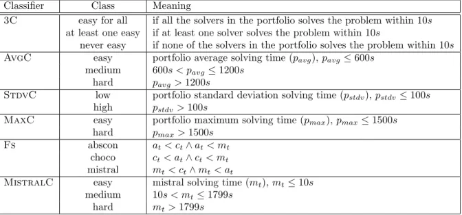
3.3 Classifiers . . . 34
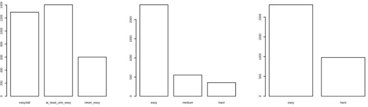
3.4 Classifiers output distribution . . . 36
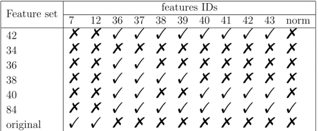
3.5 Features set . . . 37
3.6 Experimental results . . . 41
3.6.1 Comparison of different CPHydra feature sets . . . . 42
3.6.2 Comparison between CPHydra and SATzilla features sets . . 46
3.6.3 Reliability of classifiers . . . 49
4 Scheduling problems based on learning 50 4.1 Single processor case . . . 51
4.1.1 Scheduling rules . . . 52
4.1.2 Experimental results . . . 55
4.2 Multiple processors case . . . 57
4.2.1 Scheduling rules . . . 58
4.2.2 Experimental results . . . 59
4.3 The simulators . . . 64
5 Related Work 67
6 Conclusion and future work 69
Sommario
Nel lavoro di tesi qui presentato si indaga l’applicazione di tecniche di apprendimento mirate ad una pi`u efficiente esecuzione di un portfolio di risolutore di vincoli (constraint solver). Un constraint solver `e un programma che dato in input un problema di vincoli, elabora una soluzione mediante l’utilizzo di svariate tecniche. I problemi di vincoli sono altamente presenti nella vita reale. Esempi come l’organizzazione dei viaggi dei treni oppure la programmazione degli equipaggi di una compagnia aerea, sono tutti problemi di vincoli.
Un problema di vincoli `e formalizzato da un problema di soddisfacimento di vincoli (CSP). Un CSP `e descritto da un insieme di variabili che possono assumere valori ap-partenenti ad uno specifico dominio ed un insieme di vincoli che mettono in relazione variabili e valori assumibili da esse. Una tecnica per ottimizzare la risoluzione di tali problemi `e quella suggerita da un approccio a portfolio. Tale tecnica, usata anche in am-biti come quelli economici, prevede la combinazione di pi`u solver i quali assieme possono generare risultati migliori di un approccio a singolo solver.
In questo lavoro ci preoccupiamo di creare una nuova tecnica che combina un portfolio di constraint solver con tecniche di machine learning. Il machine learning `e un campo di intelligenza artificiale che si pone l’obiettivo di immettere nelle macchine una sorta di ‘intelligenza’. Un esempio applicativo potrebbe essere quello di valutare i casi passati di un problema ed usarli in futuro per fare scelte. Tale processo `e riscontrato anche a livello cognitivo umano. Nello specifico, vogliamo ragionare in termini di classificazione. Una classificazione corrisponde ad assegnare ad un insieme di caratteristiche in input, un valore discreto in output, come vero o falso se una mail `e classificata come spam o meno. La fase di apprendimento sar`a svolta utilizzando una parte di CPHydra, un portfolio di constraint solver sviluppato presso la University College of Cork (UCC). Di tale al-goritmo a portfolio verranno utilizzate solamente le caratteristiche usate per descrivere determinati aspetti di un CSP rispetto ad un altro; queste caratteristiche vengono altres`ı dette features.
La combinazione di tali classificatori con l’approccio a portfolio sar`a finalizzata allo scopo di valutare che le feature di CPHydra siano buone e che i classificatori basati su tali feature siano affidabili. Per giustificare il primo risultato, effettueremo un confronto con uno dei migliori portfolio allo stato dell’arte, SATzilla.
Una volta stabilita la bont`a delle features utilizzate per le classificazioni, andremo a risolvere i problemi simulando uno scheduler. Tali simulazioni testeranno diverse regole costruite con classificatori precedentemente introdotti. Prima agiremo su uno scenario ad un processore e successivamente ci espanderemo ad uno scenario multi processore. In questi esperimenti andremo a verificare che, le prestazioni ottenute tramite l’applicazione delle regole create appositamente sui classificatori, abbiano risultati migliori rispetto ad un’esecuzione limitata all’utilizzo del migliore solver del portfolio.
I lavoro di tesi `e stato svolto in collaborazione con il centro di ricerca 4C presso Univer-sity College Cork. Su questo lavoro `e stato elaborato e sottomesso un articolo scientifico alla International Joint Conference of Artificial Intelligence (IJCAI) 2011. Al momento della consegna della tesi non siamo ancora stati informati dell’accettazione di tale ar-ticolo. Comunque, le risposte dei revisori hanno indicato che tale metodo presentato risulta interessante.
Chapter 1
Introduction
1.1
Background
In a world where we always aim to be faster, from building better mechanics/electronics parts in order to win races, to increase the CPU performance allowing us to run appli-cations that we could only dream about years ago, most research in computing tries to push the throttle for increasing performances or decreasing the time requested for solving a specific task.
The challenge is also found in the world of constraint problems. In real life, many problems are treated as constraint problems, from train scheduling to crew scheduling of a flight company. There are also simpler examples that touch our everyday life, like the crosswords or sudoku games. Constraint problems can be formalised as constraint satisfaction problems (CSPs). A CSP is defined by a finite set of variables where each one can be associated to a domain of values. A set of constraints defines then the possible assignments of values to the variables [24].
The research in this field has been interested for quite many years, developing knowledge and new techniques. This field that worries about the solving paradigm of CSPs is called constraint programming [34]. The idea of constraint programming is that a problem is stated as a CSP and a general purpose constraint solver solves it. A constraint solver im-plements a series of techniques able to find a solution of the problem submitted, possibly in an optimal way. Nowadays many solvers exist and some of them participate to interna-tional competition with the purpose to elect the best constraint solver at the state of arts.
ronments, consists of the idea of using a set of solvers. These, combined together, try to optimize certain parameters, like minimising the solving time or maximising the number of instances solved in a determined amount of time.
The portfolio approach has been already used in different context, like for Satisfiability problems (SAT) problems [43]. SAT is a specialization of CSP, with a domain of values restricted to true and false and the constraints are Boolean formulas expressed in con-junctive normal form (conjunctions of disjunctions of literals). The previous citation is an example of integration of portfolio approach with machine learning techniques. Ma-chine learning [27] is a field of artificial intelligence that employs a series of techniques to extract knowledge, in general, from past cases and use it in future. This general ap-proach is also well known in field like cognitive science. In the portfolio case a machine learning algorithm could be useful deciding which solver to run looking on similarities of problems treated in the past.
1.2
Motivation and goals
In this work we take the challenge of creating a new way of combining a portfolio ap-proach with machine learning techniques. At the state of art the closest examples that can be found are CPHydra and SATzilla. CPHydra [30] is a portfolio for solv-ing CSPs developed at the 4C research centre in University College of Cork (UCC).1 It combines a portfolio approach with case based reasoning (CBR), a popular machine learning technique. Using similarities in past cases and partitioning CPU-Time between the components of the portfolio, CPHydra maximises the expected number of solved problem instances within a fixed time limit. The previously mentioned SATzilla [43], is a portfolio for SAT solving combined with machine learning technique which forecasts the expected solving time of a given problem.
In this thesis, we continue in this successful line of research which exploits MLA in the construction of a portfolio of CSP solver. The originality of our work is that we want to explore a different way of exploiting machine learning algorithms in a portfolio. In the specific, the goal of the new approach presented is to show that exploiting classifications on CSPs is an efficient and successful strategy able to find solutions to CSPs efficiently. A classification is a methodology that, given a series of attributes in input, is giving a prediction expressed with a number of discrete categories in output, like yes/no to classify an email spam or not spam, or easy, medium, hard to classify the difficulty of a problem. Our work is using the CPHydra attributes. These attributes used are called also features and are characteristics that describe a CSP. These features are useful to
machine learning algorithms to depict important information about the constraint prob-lem analysed. Using these features we want to create reliable and competitive classifiers.
To test that classification applied to a portfolio approach is a successful technique, we want to achieve better performance compared to a configuration employing the best sin-gle solver of the portfolio. In doing this, we want to assure that this supremacy holds both in a single processor and in a multiple processors scenario. In the single processor case we want to test the case base where our approach has to perform well otherwise any further expansion would be useless. While, in the multiple processors case we want to test that our method is scalable through a multiple CPUs scenario.
1.3
Overview
In the hereby presented work we will first focus on establishing whether CPHydra fea-tures are good. In order to do that, we will first create a group of classifiers extracted from analysis on the run time distribution of the portfolio solvers. On these classifiers, we will compare CPHydra features, after an optimization work, to the features of one of the finest portfolio solver, SATzilla[43]. We will also verify that the classifiers created are reliable by means of determined statistics.
Once the quality of the features and the reliability of the classifiers are established, in our next phase we assembles the information extracted from classifiers. This informa-tion will be used for optimising a specific statistical measure obtained solving CSPs. In our work we want to minimise the average finishing time, the time by which an instance is solved. Minimising the average finishing time can be achieved by solving each instance with an increasing order of difficulty. In the portfolio context doing this corresponds to ordering the instances accordingly to their degree of hardness and then employing the fastest solver to solve the instance. Such ordering of the instances will be consistently smart to improve the usage of the portfolio. In doing that, we want to be sure that we outperform the performances of a system composed by the best constraint solver of the portfolio: mistral [16]. This has to be verified both in a single processor case and a mul-tiple processor case for establishing that our solution scales correctly in a parallel setting.
The work here presented is structured in the following way: Chapter 2 will introduce the background concepts about machine learning, constraint satisfaction problems, con-straint programming and portfolio approach. Chapter 3 will go into the learning part, talking about the classifiers built, features selection, and features set comparison. Chap-ter 4 will consider the second main part of the work, where we will build scheduling rules
in Chapter 5 we will survey some related works before concluding and discussing future works in Chapter 6.
The hereby presented work resulted to a paper submission to the 2011 International Joint Conference of Artificial Intelligence (IJCAI).2 By the time of submitting the thesis
we are not yet informed about its acceptance status. However the reviewers feedback has revealed that our method is appealing. The submitted paper is a result of a collaboration with the 4C research centre in University College of Cork.
Chapter 2
Background
In this chapter, the required background on the thesis work is provided. However, due to the vastness of each topic treated, this chapter will be focus only on the aspects which are necessary for understanding of the presented work. The background chapter consists of an introduction to machine learning and its algorithms; a section reserved to introduce constraint satisfaction problems and constraint programming paradigms and a section introducing the principles of algorithm portfolio.
2.1
Machine learning
Since the creation of computers, there was always interest in making the machines learn and make them able to acquire knowledge from the environment. Starting from the sci-fi film category, through the Isaac Asimov literature, many aspects about robotics and machine learning were covered, mainly for entertainment purpose (robots turning against the human beings). The reality is far away from the Hollywood point of view.
Nowadays, the fields in which learning techniques are applied are many and not related only to computer science. In the following we present some examples.
Games: there are several papers related to the topic of making a machine learn how to play chess against human and competing on the better intelligence. Since then, all the video games started to develop better learning agents/players. Such an example can be found in a particular field called general game playing. In [8] an agent is developed with the aim of create an intelligence that can automatically and in real-time learn how to play many different games at an expert level without any human intervention.
Robotics: many are the aspects where learning in robotics is important. Depending on the purpose of the robot, there could be learning algorithm regarding interaction skills, working procedures. The classic example is the vacuum cleaner that analyses its previous behaviour for taking further decision, like clean first a particular spot which is usually dirty or either learn over obstacle objects [36].
Biology and medicine: there are numerous cases [28] [21] in which learning is required in these fields, for example predicting various form of cancer like prostate cancer or women breast cancer [2] and for measuring the DNA microarrays expression [15]. These DNA microarrays evaluate the eventual presence of a specific gene in a given cell and, if affirmative, the presence of a determined molecule in it .
Business: interesting applications are the predictions of important parameters like risk factors for loans or bankruptcy [26]. Among the others there are specific works on agent learning, for example, on oligopolistic competition in electricity auctions [13].
This section continues with an introduction on the main type of learning, a distinc-tion between lazy and eager learning, as well as a list of the main machine learning algorithms and performances metrics used to evaluate the results produced.
2.1.1
Supervised, unsupervised and reinforcement learning
Before taking a step further, let us give a formal definition of learning according to Mitchell’s “Machine Learning” [27]:
A computer program is said to learn from experience E with respect to some class of tasks T and performance measure P, if its performance at tasks in T, as measured by P, improves with experience E.
Let us take a concrete example. Imagine a software able to recognize handwritten digits for the ZIP code. The task T, that the software has to accomplish, is to recognize the handwritten digits from the image provided. The so called experience E is a database of images containing digits and respectively the output result from which the software will analyse similarities, patterns and learn. The performance P measure is given by the percentage of images correctly recognized by the software.
This is a classic example of a supervised learning problem. Such a problem is easily identifiable by a set of variables in input, measured or given, that are having influences on the output(s). The word supervised is referred to the goal which is to use inputs to
predict the output values. This type of learning is often referred as “learning with a teacher” [15]. Under this metaphor the “student” presents an answer ˆy for each xi in the
training sample, and the supervisor or “teacher” provides either the correct answer yi
and/or an error associated with the student’s answer. This error is usually characterized by some loss function L(y, ˆy), for example, L(y, ˆy) = (y − ˆy)2.
Examples such as handwritten digit recognition or spam recognition in emails, in which the aim is to assign a finite number of discrete categories (i.e. given an email classify it spam or not spam), are called classification problems. If the searched output consists of one or more continuous variables, then the task is called regression. A discrete value can assume only a finite set of values, while a continuous can assume infinite different values. An example of a regression problem is the prediction of the prostate-specific antigen (PSA) value. Such a continuous value for example, measures the proteins produced by cells of the prostate gland in the blood. The higher this values is, the more likely it is that this specific cancer is present.
With a bit more of formality, it can be said that, given a vector of input data X, where X = x0, ..., xn, a machine learning algorithm (MLA) is a function f that returns
a so called prediction ˆY.
f (X) = ˆY
If the output is discrete, the function f is called classifier, otherwise regression, if the output is continuous.
In other pattern recognition problems, the training data consists of a set of input vectors without any corresponding target values. Such problems are called unsupervised learning problems [15]. Their goal may be to discover groups of similar examples within the data (clustering), or to determine the distribution of data within the input space (density estimation). This type of learning is done without the help of a supervisor or teacher providing correct answers or a degree of error for each observation, that is why is also known as “learning without a teacher”. The previously introduced DNA microarrays expression is an example of unsupervised learning problem, since a DNA microarrays expression does not need to be in a class, but it needs to be clustered or analysed in other expressions so that patterns might be found.
The last of the most famous learning type, which is used in applications like the afore-mentioned robotics, is the reinforcement learning. This technique [3] is interested in the problem of finding suitable actions to take in a given situation in order to maximize a
learning process comes from examples provided by some knowledgeable external super-visor that alone is not adequate for learning from interaction [39].
These activities can be easily summarised in the following statements. A reinforce-ment learning agent and its environreinforce-ment interact over a sequence of discrete time steps. The specification of their interface defines a particular task: the actions made by the agents are the choices, the states are basis for making the choices and the rewards are the basis for evaluating the choices made. Everything inside the agent is completely known and controllable by the agent while everything outside is incompletely controllable but may or may not be completely known. Given a stochastic rule by which the agent selects actions as a function of states (a policy), the agent’s goal is then to maximize the amount of reward it receives over time and choices made.
There is one feature that is worth to be mentioned about reinforcement learning which regards exploration and exploitation. It is very important, in fact, to monitor the trade-off between exploration, in which the system tries out new kinds of actions to see how effective they are, and exploitation, in which the system makes use of actions that are known to yield a high reward. It has to be a balanced choice between the two because being too strongly focused on either exploration or exploitation will bring poor results [39].
2.1.2
Lazy and eager learning
Lazy methods are called in such way because they defer the decision of how to generalize beyond the training data until each new query instance is encountered. On the other hand, methods that are called eager generalize beyond the training data making possible all the operations that define the approximation of the algorithm to the target function before observing the new query [27].
Let us distinguish two differences between lazy and eager learning: • in computation time;
• in the classifications produced for new queries.
In the first case, lazy methods will generally require less computation time during train-ing, but more computation time when they have to predict the target value for a new query. In the second, lazy methods may consider the query instance xq, when deciding
how to generalize beyond the training data. While, in the eager methods, by the time they observe xq, they have already chosen their (global) approximation to the target
function. In other words, a lazy algorithm might take decision at the querying time, while an eager algorithm cannot.
2.1.3
Machine learning algorithms
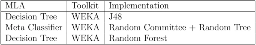
The list of machine learning algorithms (MLA) implemented so far is very long and some of them require advanced mathematical/statistical background to be completely clear. The purpose of this section, is to give an overview of the most important MLA oper-ating mainly in supervised learning, since the thesis work is interested on these kind of learning problems. For the sake of simplicity the algorithms are grouped in the closest manner possible to the categorization method of Weka [17], a data mining tool used for this project.1
The principal categories are the following: • artificial neural networks;
• Bayesian learning methods; • decision trees;
• lazy learners; • meta classifiers; • regression; • rules;
• support vector machine.
Artificial Neural Network (ANN) [27] is a method that tries to resemble to the human neural network. The most famous type of ANN, multi layer perceptron, is based on the perceptrons, the artificial equivalent of the neurons. Artificial neural networks are built out of a densely interconnected set of perceptrons, where each one of them takes a number of real valued inputs (possibly the outputs of other units) and produces a sin-gle real valued output (which may become the input to other units). These inputs and outputs influence the interconnected perceptrons making the neural network adaptive to the training inputs. ANN can be a powerful tool but is usually complex to find a good tuning of the parameter and also they require a long training time.
In the Bayesian [27] learning methods, the algorithms are based on the Bayes formula, which determines the most likely hypothesis from some space H, given an observed
1
training data set D. The Bayes formula specifies a way to calculate the probability of an hypothesis h in the following way:
P (h|D) = P (D|h)P (h) P (D)
where P (h), called the prior probability of h, measures the probability of the correctness of the hypothesis h, before having seen the training data. P (D) denotes the probability that training data D will be observed. P (D|h) denotes the probability of observing data D knowing that the hypothesis h is valid or holds. P (h|D) is the posterior probability of h and it reflects a level of confidence on h holding after the training data D is seen. A re-mark is that the posterior probability P (h|D), in contrast to the prior probability P (h), is influenced by the training data D. Among the variety of Bayesian learning methods one worth to be mentioned is the naive Bayes learner. In some domains its performance showed to be comparable to that of neural network and decision tree learning [25].
Decision trees algorithms, like the name says, are methods that construct a tree eas-ily readable following the branching sequence that, from the root node to the leaf node, leads to a classification decision [27]. Each node of the tree specifies a test of some attribute of the instance, while each tree branch from a node, corresponds to one of the possible values of this attribute. Decision trees usually work with entropy evaluation once it comes to select which attribute branch first and are the most direct example of eager learning type. An example of classic decision trees is C 4.5 [33].
Decision trees are nowadays brought to a powerful form of classification called Ran-dom Forest [4]. This algorithm uses the technique known as bagging. This method works by training each algorithm employed, in this case random trees, on a sample cho-sen randomly from the original training set. The multiple output computed are then combined using simple voting. The final composed output classifies an example x to the class most often assigned by the underlying multiple output previously computed. In general, decision trees are algorithms that suit better for classification problems [27].
In the lazy learning category, discussed above, the most important algorithm is k-NN. The k-nearest neighbor [15] is a lazy learning algorithm that returns the k most similar cases to the new problem submitted, where k is a parameter of the algorithm. To define how to evaluate the similarity between the cases, a metric is required, which normally is the Euclidean distance.
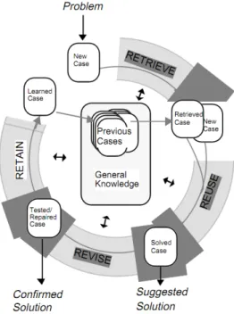
Case based reasoning (CBR) [1] is a lazy learning method that allows to elaborate solu-tions of new appearing problems, choosing from similar cases already encountered and solved. An important feature is that CBR is an approach to incremental, sustained learn-ing, since a new experience is retained each time a problem has been solved, making it
immediately available for future problems. Generally the CBR activities are summarized by the following list:
1. Retrieve the most similar cases;
2. Reuse the information and knowledge in that case to solve the problem; 3. Revise the proposed solution;
4. Retain the parts of this experience likely to be useful for future problem solving.
Figure 2.1: CBR: the cyclic process.
In Figure 2.1 the typical cyclic process of a CBR is depicted. The new problem is submit-ted to the CBR which, with the help of a k-nearest neighbor (k-NN) algorithm, retrieves the similar cases. Such similar cases combined sometimes with general knowledge are being reused for producing a solution of the problem submitted. Through the revise process the solution is then validated and corrected if the process is not successful. The last phase of retaining consists in extracting the useful information able to increase the cases database for the future usage.
This is not completely true. Even if there are similarities in these approaches, there is a substantial difference in the way they are learning. CBR uses the knowledge of the past cases, or in some cases the general world knowledge, while reinforcement learning techniques acquire knowledge exclusively by means of a process of trials and errors.
In the meta classifiers family there are all those algorithms powered by an inner MLA combined with techniques like bagging, boosting or wagging. Some examples of meta classifiers are AdaBoost, MultiBoost and Random Committee. To describe the main idea of these classifiers, let us analyse briefly AdaBoost. AdaBoost [9] is based on the tech-nique of boosting. Such a method works by repeatedly running a given weak learning algorithm on various distributions over the training data, and combining the classifiers produced by the weak learner into a single classifier. More specifically, AdaBoost calls the weak learn algorithm (WL) repeatedly in a series of rounds. On each round, Ad-aBoost provides WL with a distribution over the training set. In response, WL computes a classifier or hypothesis which should correctly classify a fraction of the training set that has large probability with respect to. The weak learner’s goal is to find an hypothesis which minimises the training error. At the end of the rounds AdaBoost combines the weak hypotheses into a single final one. The difference between AdaBoost (mainly the boosting methods) from a bagging technique is that boosting is iterative. Whereas in bagging individual models are built separately, in boosting each new model is influenced by the performance of those built previously. Another important advantage coming from the iterative nature is that boosting allows weighting a model’s contribution by its per-formance rather than giving equal weight to all models, like in bagging.
MultiBoost [40] is actually an extension of AdaBoost that combines AdaBoost with wag-ging. Wagging is variant of bagging, which requires a base learning algorithm that can utilize training cases with differing weights. Rather than using random samples to form the successive training sets, wagging assigns random weights to the cases in each training set. Random Committee [41] builds an ensemble of weak classifiers and averages their predictions. Random Committee distinguishes itself by making each classifier be based on the same data but using a different random number seed. This only makes sense if the base classifier is randomized, otherwise the classifiers would all be the same.
The simplest algorithm of regression category is the linear regression [27]. Such an algorithm approximates a linear function f to a given set of training samples close to the query instance x.
f (x) = w0+ w1a1(x) + w2a2(x) + . . . + wkak(x)
In the specific, ai(x) indicates the ith attribute value of the instance x, while wi are the
coefficients weighting each attribute. This is a natural technique considered when the class and all the attributes are continuous values.
In the rules category are grouped all those classifiers based on simple rules [18], like 1-R, a classifier that learns one rule from the training set.
A Support Vector Machine (SVM) is a method that aims to find the optimal sepa-rating hyperplane that separates the instances of a two classes problem (separable or not). In order to find this optimal solution, SVM uses a margin, defined as the smallest distance between the decision boundary and any instance of the training set. SVM then, separates the two classes’ problem, maximising the margin between the training points and the decision boundary.
SVM is not the only algorithm that is separating the classes. For example the multi layer perceptron algorithm, introduced under the ANN category, tries to find a separat-ing hyperplane minimizseparat-ing the distance of misclassified points to the decision boundary. However this solution is dependent on the initial parameter of the perceptrons and the solution is found just one of the many available. SVM has different variants, like the one that can be applied to regression problems or for example the MultiClass SVM that allows the algorithm to manage classification with multiple classes since the classic SVM is meant to be for two classes problems only [15].
2.1.4
Performances metrics and testing techniques in
classifi-cation
There are many metrics able to depict the goodness of a classification in the supervised learning context, but without a doubt the first one that has to be considered is the accuracy. The accuracy of a machine learning algorithm represents, in percentage, how many instances are correctly classified.
Another metric, Cohen’s kappa statistic (κ-statistic) [5] is used to measure the agree-ment between the predicted and the observed classification. It is expressed with a value from 0 to 1, where values closer to 0 represent a poor agreement, while values closer to 1, a good agreement. However, this measure does not take misclassification costs into account.
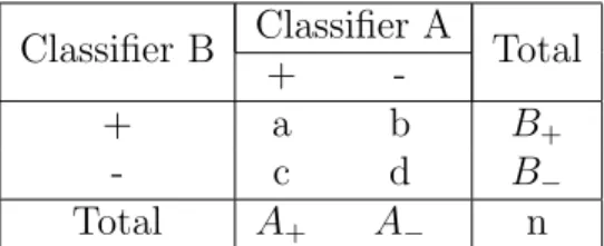
Now we will show a practical example using an outcome from an experiment like the one used in [14]. In Table 2.1 two type of classifiers ( A,B) classify n instances in two classes + and −. a and d represent the number of instances classified respectively + and - from both classifiers A and B. b and c, instead, represent the number of instances which are
Classifier B Classifier A Total +
-+ a b B+
- c d B−
Total A+ A− n
Table 2.1: Distribution of n instances classified by two classifiers.
The formula of Cohen’s κ-statistic is the following:
κ = P (a) − P (e) 1 − P (e)
where the probability of agreement (meaning that both classifiers have the same output) P (a), is defined as:
P (a) = a + d n
the probability of expected agreement P (e) is defined as follows:
P (e) = P (A+)P (B+) + P (A−)P (B−) and P (A+) = A+ n , P (B+) = B+ n , P (A−) = A− n , P (B−) = B− n
In the Tables 2.2 and 2.3 two examples that show how κ is varying through different data are given. Let us take the following tables with both n = 100 instances over two classes and two classifiers (the problem can be extended to multiple classes):
Classifier B Classifier A Total +
-+ 45 15 60 - 25 15 40 Total 70 30 100
Table 2.2: κ statistic calculation example with 100 instances.
P (a) = 45 + 15 100 = 0.6 P (e) = 0.7 × 0.6 + 0.3 × 0.4 = 0.42 + 0.12 = 0.54 κ1 = 0.6 − 0.54 1 − 0.54 = 0.1304
Classifier B Classifier A Total +
-+ 25 5 30
- 5 65 70
Total 30 70 100
Table 2.3: κ statistic calculation example with 100 instances.
P (a) = 25 + 65 100 = 0.9 P (e) = 0.3 × 0.3 + 0.7 × 0.7 = 0.09 + 0.49 = 0.58 κ2 = 0.9 − 0.58 1 − 0.58 = 0.7619
In Table 2.2, the level of disagreement is higher than the one in Table 2.3 and is testified by their κ values: κ2 = 0.7619, κ1 = 0.1304.
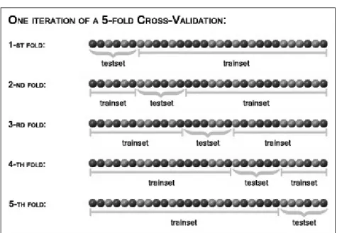
The most important testing technique in classification is the n-fold cross validation [27]. A cross validation is a methodology that consists of dividing the original data set in n-folds (typically 5 or 10). Iteratively then, one fold is kept as testing set while the remaining n − 1 folds are used for training the classifier. The cross validation is usually adopted whenever the data set is not big enough to allow two consistent sets, one for training and the other one for testing. Furthermore it might be useful to reduce the problem of overfitting which happens usually in the decision tree learning when there is noise in the data (wrong instances) or when the training set is too small for having a good representation of the problem. An algorithm is said to be overfitting when an increase of performance of the classifier on the training set, corresponds to a decrease on the test set. This results in taking the training data too much as a strict example of reality, risking that the algorithm is not able to later generalize on new presented problems. An evident drawback of cross-validation is that the number of training runs required are increasing as a factor n and this can be problematic for those models that are computationally expensive to train.
Figure 2.2: An example of a 5-fold cross validation.
The Figure 2.2 gives an example of 5-fold cross validation where each fold consists of six instances represented as dots.2 As it is possible to see, in the first iteration only first
fold is kept as test set, while the remaining ones are used as the training set. Once it iterates over the next fold, the fold is selected as new test set. This process continues until all the five folds are considered.
2.2
Constraint satisfaction problems and constraint
programming principles
In this section we will focus on the basic principles of constraint satisfaction problems, giving an overview from the theoretical point of view, introducing also one of its special case, the satisfiability problems. Then, we will present some basic concepts of constraint programming and some principles and examples of constraint solvers.
2.2.1
Constraint satisfaction problems
The every day life is full of constraint problems. When it comes to scheduling trains or scheduling crews for a flight company, these are all problems that deal with constraints. Even in the everyday games, like crosswords and sudoku, we can find constraints prob-lems. Given a real world constraint problem, it is necessary to define a mechanism that
allows to formalize the problem in a schematic way.
Such problems can be formulated as Constraint Satisfaction Problem (CSP), defined in the Handbook of constraint programming [34] as:
A CSP P is a triple P = hX, D, Ci where:
• X is an n-tuple of variables X = hx1, x2, . . . , xni;
• D is a corresponding n-tuple of domains D = hD1, D2, . . . , Dni such
that xi ∈ Di;
• C is a t-tuple of constraints C = hC1, C2, . . . , Cti.
A CSP is defined by a finite set of variables, each of which is associated with a domain of possible values that can be assigned to the variable, and a set of constraints that define the set of allowed assignments of values to the variables [24]. A constraint Cj
is a pair hRSj, Sji where RSj is a relation on the variables in Sj. In other words, each
constraints Cj involves some subset of the variables Sj and specifies in RSj the set of
allowed combinations of values that the variables can take simultaneously. In such way, RSj can be defined as a subset of the Cartesian product of the domains of the variables
in Sj.
Given a CSP, the task is normally to find an assignment to the variables that sat-isfies the constraints, which we refer to as a solution. A solution P is an n-tuple A = ha1, a2, . . . , ani where ai ∈ Di and each Cj is satisfied in that RSj and it holds
the projection of A onto the scope Sj .
Given a CSP, it is requested to find one of the following: • any solution, if one exists;
• all the solutions;
• an optimal solution given some objective function defined in terms of apart or the entire set of variables.
A classic example used in literature: the n-queens problem. Such a problem consist of finding the right disposal point of n queens on a n × n chessboard, in a way that each queen is not able to attack and being attacked by another one (considering that a queen moves horizontally, vertically and diagonally).
One possible way to encode this problem as CSP is as follows: • a variable xi is defined for the queen on row i;
• the domains Di of each variable xi is defined as Di = {1 . . . n}, giving the possible
columns that queen i can be placed;
• ∀i, j, i 6= j having 1 ≤ i < j ≤ 8, the constraints are defined as:
1. xi 6= xj (knowing that two queens cannot be on the same row from the i 6= j,
here we say that two queens cannot be placed on the same column);
2. i − j 6= xi− xj (no other queen can be placed on one of the two diagonals);
3. j−i 6= xj−xi(no other queen can be placed on other one of the two diagonals).
Figure 2.3 shows one of the possible solutions of the 8 × 8 queens problem. It is verifiable that no queen on the board is able to attack another one.
Figure 2.3: One possible solution of the 8-queens CSP.
Another example that helps to better understand what CSPs are, is the popular sudoku game. A classic sudoku problem [37] can be expressed in the natural language like the following: given a 9 × 9 board, the purpose of the game is to fill each of the 81 boxes with a number from 1 to 9 in a way that in each row, in each column and in each 9 major 3 × 3 subregion, is possible to have all the numbers from 1 to 9. An solution of a sudoku game looks like the following:
2 5 8 7 3 6 9 4 1
6 1 9 8 2 4 3 5 7
4 3 7 9 1 5 2 6 8
3 9 5 2 7 1 4 8 6
7 6 2 4 9 8 1 3 5
8 4 1 6 5 3 7 2 9
1 8 4 3 6 9 5 7 2
5 7 6 1 4 2 8 9 3
9 2 3 5 8 7 6 1 4
One possible way to encode this problem as CSP is as follows:
• each variable xi,j corresponds to the cell on the board, with i, j ∈ [1, 9];
• the domain D(xi,j) = {1 . . . 9}, giving the numbers that can be filled in each cell;
• and the constraints are :
1. ∀i, j1, j2 ∈ [1, 9], then xi,j1 6= xi,j2 (two numbers in the same row cannot be
equal);
2. ∀j, i1, i2 ∈ [1, 9], then xi1,j 6= xi2,j (two number in the same column cannot be
equal);
3. for each 9 subregions Sr, xij 6= xhk, if i, j, h, k ∈ Sr, i 6= h and j 6= k (two
numbers in the same major 3 × 3 subregion cannot be equal).
The arity of a constraint is the number of variables it constrains. This is an impor-tant feature that can be used for analysing and depicting the specificity and possibly the complexity of CSP. A first classification among CSP comes precisely on this fea-ture. Constraints are defined as: unary, binary or n-ary if the arity is equal to 1, 2 or > 2 respectively. Intensional constraints are specified by a formula that is the charac-teristic function of the constraint. Extensional constraints are specified by a list of its satisfying tuples. Global constraints are those constraints that involve relations between an arbitrary numbers of variables. The most used example of a global constraint is the all-different constraint which states that the variables in the constraint must be pairwise different [34].
2.2.2
SAT
Satisfiability problems (SAT) are actually a specialization of CSP, where the domains are restricted to be {true, f alse} and the constraints are clauses expressed as a Boolean formula in conjunctive normal form (CNF) [34].
An example of a SAT problem can be the following: the formula (¬x1∨ x2) ∧ (x1 ∨ x3)
is a clause expressed in CNF, conjunction of disjunction of literals, where a literal is a Boolean variable or its negation. A solution to this problem is: x1 = F ; x2 = F ; x3 = T .
The satisfiability of propositional formulae is one of the most famous example of prob-lems in computer science, mainly because of its interesting applications in the theoretical field. It has been proved that problem in the N P class [6] (problems for which exist an algorithms that given an instance i and one of its possible solution s, is possible to verify the correctness of s within a polynomial time) can be encoded into SAT ones and then be solved by SAT solvers.
2.2.3
Constraint programming
Constraint programming is a solving paradigm of constraint problems that draws on a wide range of techniques from artificial intelligence, computer science, databases, pro-gramming languages, and operations research. Constraint propro-gramming is currently applied with success to many domains like:
• scheduling; • planning;
• vehicle routing (i.e. the travelling salesman problem (TSP): the problem of finding the shortest path that visits a set of customers and returns to the first one); • configuration (the task of composing a customized system out of generic
compo-nents. Classic examples involve constraints to assembling computers and cars); • networks (apart from the classic networking field, CP can be used in
electric-ity/water/oil networks); • bioinformatics.
Constraints are just relations, and a constraint satisfaction problem (CSP) states which relations should hold among the given decision variables. For example, in scheduling activities in a company, the decision variables might be the starting times and the du-rations of the activities and the resources needed to perform them, and the constraints might be on the availability of the resources and on their use for a limited number of
activities at a time.
The basic idea in constraint programming is that the user states the constraints and a general purpose constraint solver is used to solve them. Constraint solvers take a real-world problem like the scheduling activities in a company previously mentioned, represented in terms of decision variables and constraints, and find an assignment to all the variables that satisfies the constraints.
2.2.4
Constraint solvers
Constraint solvers search the solution space using different techniques [34]. The main algorithmic techniques for solving CSPs are backtracking search, and local search. While the first one is an examples of complete algorithm, the local search is an example of in-complete algorithm. Complete means that there is the guarantee that a solution will be found, if one exists, otherwise prove unsatisfiability, or find an optimal solution. On the other hand incomplete algorithms are those that cannot assure to find a solution. Systematic methods, like the more advanced versions of backtracking search, interleave search and inference, which helps detect regions of the search space that does not con-tain solutions. This information is usually propagated among the constraints. Constraint propagation explicitly forbids values or combinations of values for some variables of a problem because a given subset of its constraints cannot be satisfied otherwise. For ex-ample, in a crossword puzzle, you propagate a constraint when the words Iceland and Germany are discarded from the set of European countries that can fit a 7-digit slot because the second letter must be a ’R’. The backtracking search is represented as a search tree where partial solutions are built up by choosing values for variables until a dead end is reached, where the partial solution could not be consistently extended. When the dead end is reached, the last choice is rolled back and another one tried (back-track). This is done in a systematic manner that guarantees that all possibilities are tried.
A local search algorithm starts with an initial configuration (for the CSP are, typically a randomly chosen, complete variable assignment), in each step the search process moves to a configuration selected from the local neighbourhood (typically based on heuristics function). This process is iterated until a termination criterion is satisfied. To avoid stagnation of the search process, almost all local search algorithms use some form of randomisation, typically in the generation of initial positions and in many cases also in the search steps. Local search algorithms cannot be used to show that a CSP does not have a solution or to find an optimal solution. However, such algorithms are often effec-tive at finding a solution if one exists and can be used to approximate an optimal solution.
tion in 2009.3 However, in this competition only solvers capable of accepting a CSP with the specific XML format, XCSP [35] are admitted. The results are ranked based on the number of solved instances and ties are broken by considering the minimum total solution time. Based on this criteria of ranking, Figure 2.4 shows the results of the 2009 competition. Among the participating solvers pcs, abscon, choco, sugar and mistral are winners in one or more category. In the specific mistral and sugar are tied winner with both 8 leading categories over 21, then choco and abscon won 2 and pcs 1.
Figure 2.4: The winner of the 2009 constraint solver competition.
Unfortunately no direct ranking is provided on the “speed” of the solvers or at least on the ratio between CPU time and number of solved instances.
As well as constraint solvers, SAT solvers state of art is presented in different com-petition like the International SAT Comcom-petition 4 and the SAT Race. At the writing
time the last competitions held are in 2009 for the SAT competition 5 and 2010 for the SAT Race. 6 The variety of SAT solvers participating at these competitions are high and the categories of competition are split on type of instances, representation of problems or type of execution.
3http://www.cril.univ-artois.fr/CPAI09/ 4http://www.satcompetition.org/ 5http://www.satcompetition.org/2009
From the 2009 SAT competition, 9 are the categories in which the solvers are tested. Among the competing solvers, the portfolio solver SATzilla won 3 out of 9, clasp 2 categories and precosat , glucose, TNM and March hi one.
From the 2010 SAT race, among the participating solvers, the winners of the three competitions are CryptoMiniSat, plingeling and MiniSat++ 1.1.
It is interesting to see how SATzilla is employing the best performing solvers of the 2006 SAT race and 2005 SAT competition for winning three categories both in the 2007 and 2009 SAT competition. This portfolio of SAT solvers will be described in Section 2.3.1.
2.3
Algorithm portfolio
Over the past decade there has been a significant increase in the number of solvers that have been deployed for solving constraint satisfaction problems. It is recognised within the field of constraint programming that different solvers are better at solving different problem instances, even within the same problem class [12]. It has been shown in other areas, such as satisfiability testing and integer linear programming that the best on av-erage solver can be outperformed by a portfolio of possibly slower on avav-erage solvers, examples are respectively SATzilla [43] and this work [23]. The same philosophy is applied also to some latest machine learning algorithms, like the previously mentioned AdaBoost (Section 2.1.3). Instead of using a single classifier, a series of ”weak” classifiers are combined together in a way to reach a consensus. The portfolio selection process is usually performed using a machine learning technique based on feature data extracted from constraint satisfaction problems.
Portfolio solvers are often distinguished by the following categorization: • parallel, where all the solvers all run in parallel;
• sequential, where a solver waits for the previous one to finish, before starting its computation;
• partly sequential, an hybrid version of the previous categories.
Two portfolio solvers are involved in the hereby presented work. CPHydra is the protagonist portfolio solver. From which, we extract the features to manipulate. The
2.3.1
SATzilla
SATzilla [43] is an automated approach for constructing per-instance algorithm se-quential portfolio for SAT problems. SATzilla uses machine learning techniques, such as linear regression, to build run time prediction models based on features computed from instances.
In the specific, the original version of SATzilla uses a very specific strategy for building a sequential portfolio. The part of construction is done offline. After selecting a set of in-stances believed to be representative of some underlying distribution, SATzilla selects a set of candidate solvers that are expected to perform well on the data distribution. The appropriate features are then selected on these problem instances. This operation is usually done with the help of knowledge from a domain expert. The features set are calculated on a training set of instances, determining also the real running time for each algorithm candidate.
In the next phase SATzilla identifies one or more solvers that have to be used as pre-solvers. Such solvers are used to eliminate those problems that are solved in a short amount of time and will be launched before the feature computation. Using a validation dataset, SATzilla then determines the backup solver. This solver is the one which achieves the best performances on those instances that are not solved by the pre-solvers. In absence of instances that go timeout or produce error, the best single solver known so far is selected as backup solver. Then a model containing the runtime predicted for each solver is constructed and SATzilla selects the best subset of solvers to use in the final portfolio.
In the online phase, SATzilla runs the pre-solvers for a limited amount of time; if the pre-solvers succeed the process end up here but if the pre-solvers fail to solve the problem then it computes the features of the instance just run. If, once again, these fea-tures are not calculated because of errors or timeout, then the backup solver is used for solving the instance. If instead the features are calculated, then the runtime algorithm is predicted using a simple variant of linear regression and finally, once the best predicted is selected, this is run. In the International SAT Competition 2009, SATzilla won all three major tracks of the competition.7
2.3.2
CPHydra
CPHydra [30] is sequential portfolio solver for constraint satisfaction problems devel-oped at 4C (Cork Constraint Computation Centre) that uses a CBR machine learning algorithm to select solution strategies for constraint satisfaction. A CBR methodology
performs well in decision making as reported in [11]. CPHydra was the overall winner of the 2008 Constraint Solver Competition. Its strength relies on the combination of machine learning methodology, case based reasoning (CBR), with the idea of partition-ing CPU-Time between components of the portfolio in order to maximise the expected number of solved problem instances within a fixed time limit. Mainly because it has been built for the 2008 competition, CPHydra uses a portfolio with three solvers (abscon, choco and mistral ) and it does not exploit the latest results of the competition, where sugar won the same number of categories as mistral. However, comparing mistral to the other solvers will clearly establish that it is the fastest solver in the portfolio.
In the retrieval phase of the CBR, CPHydra uses a k-nearest neighbor algorithm that returns the set of solving times for each of the k most similar problem instances found in the base case along with their similarities to the submitted one. In order to define how to evaluate the similarities between the cases, CPHydra uses a classic Euclidean distance between the features of the problems. In situation of equality, tied cases are returned in the k neighbour. In the reuse phase the runtime of the k most similar cases are used to generate a solver schedule. For each problem submitted, γ are the similar cases returned. For a given solver s and a time point t ∈ [0 . . . 1800], we define C(s, t) as the subset of γ solved by s given at least time t. The goal of the scheduler is then to maximise C(s, t), for each solver. This goal is then optimised weighting the input case by the Euclidean distance of each similar case.
During the revision phase a solution is evaluated and validated running each solver for the amount of time decided by the scheduler. If only one solver solves the instance within the time slot, then the schedule is considered a success. A revision of the solution is not possible in a competition scenario, where there would not be enough time for run-ning each solver. In the retention phase, as well, there is not enough time for building the complete new case. Such an operation requires to run every solver till a solution is reached and in competition scenario this is not possible.
The experiments and the 2008 competition results showed that CPHydra is implement-ing a winnimplement-ing strategy. In the 2008 competition, CPHydra was the overall winner.8
Chapter 3
Learning from problem features
Learning is a generic concept that can be applied to many fields. Hereby, the learning concept will be applied to CSPs for information extraction. This information is going to be useful for solving CSPs in the context of a portfolio solver, as will be explained in Chapter 4.
Next we will first introduce the dataset used. Then we will analyse how the portfolio is behaving on this dataset. We will tackle the solving times of each solver for building a group classifiers. With these classifiers we will perform two kinds of tests: one to test different features set of CPHydra and the other one to compare the CPHydra features to those of SATzilla. The latter test will establish how reliable our classifiers are.
In order to avoid confusion, in the next sections we will talk about instance or prob-lem, indicating a CSP instance.
3.1
The international CSP competition dataset
The comprehensive dataset of CSPs used is based on the various instances from the annual International CSP Solver Competition from 2006-2008. Overall, there are five categories of benchmark problems in the competition:
• 2-ARY-EXT instances involving extensionally defined binary (and unary) con-straints;
• N-ARY-EXT instances involving extensionally defined constraints, at least one of which is defined over more than two variables;
• N-ARY-INT instances involving intensionally defined constraints, at least one of which is defined over more than two variables;
• GLB instances involving any kind of constraints, including global constraints. The competition stated that a problem would have to be solved with a time out value of 1800 seconds. Once the time frame is passed, the problem is considered not solved. So, in the dataset considered, it is clear to see whether or not a solver finds a solution before the cut off. Another important remark is that, at the competition time, the problems that are not solved by the portfolio within 1800 seconds of cut off, are removed from the dataset. In total, the dataset contains approximately more than 4000 instances across these various categories. Later we will restrict this dataset to a subset of 3293 for reasons that we will clarify.
3.2
Portfolio solving time analysis
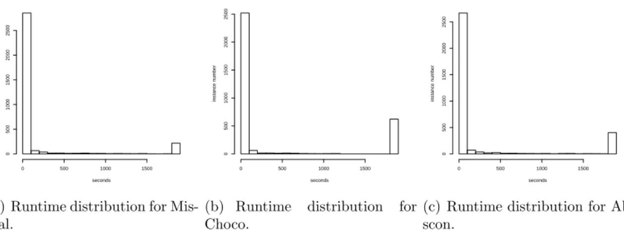
Based on the three solvers of the portfolio used in the 2008 CSP Solver Competition variant of CPHydra, it is interesting, as a first step, to present the runtime distribu-tions. Figures 3.1(a), 3.1(b), 3.1(c), respectively mistral, choco and abscon solving time distributions, are introducing their distributions. Each runtime distribution is specified as a histogram of the frequency (y-axis) of a given runtime (x-axis). The purpose of doing this is to show for every single solver in the portfolio, the number of instances of the dataset solved in the given time windows. This can highlight the fact that there are many instances for which one of the solvers finds a solution quickly, while another solver struggles to solve them. However, it is not the case that each solver finds that the same instances are either easy or hard because. For instance, abscon can solve some instances in an easier way than mistral and the situation is the other way around in some other instances. This is a good hint for developing what will be one of the first classifiers, which however will be more useful in the scheduling part: a classifier which will try to forecast the fastest solver in the portfolio.
seconds instance n umber 0 500 1000 1500 0 500 1000 1500 2000 2500
(a) Runtime distribution for Mis-tral. seconds instance n umber 0 500 1000 1500 0 500 1000 1500 2000 2500
(b) Runtime distribution for Choco. seconds instance n umber 0 500 1000 1500 0 500 1000 1500 2000 2500
(c) Runtime distribution for Ab-scon.
Figure 3.1: The performance of each solver in the portfolio on the dataset.
We note in Figure 3.1(a) that mistral seems to be the fastest solver only analysing the bars of the plot. In fact it is the one with the higher bar on the left side and lowest bar in correspondence of the timeout value.
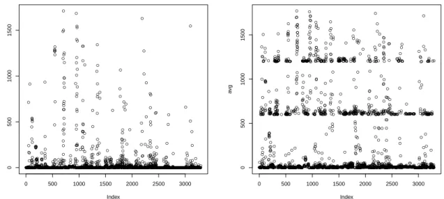
After showing how the single solvers of the portfolio are behaving, it is interesting to ad-dress directly the portfolio itself. For each instance, we extract the minimum, maximum and the average runtime of the instances given by the three solvers in the portfolio, as well as the standard deviation. Analysing such data could highlight any kind of clus-tering or distribution patterns showed by the combination of the solvers. A cluster or a distribution pattern in the plot, would manifest that a good machine learning classifica-tion could be created.
In the plots below (Figures in 3.2) we show the output distribution of data analysed. All the functions applied show a natural clustering of the instances, except the minimum. In fact the minimum plot (Figure 3.2(a)) shows a distribution that does not indicate any immediate clustering or possible classification.