Image enhancement for a Bose-Einstein condensate interferometer

(1)

Alma Mater Studiorum · University of Bologna

School of Science

Department of Physics and Astronomy Master Degree in Physics

Image Enhancement for a Bose-Einstein

Condensate Interferometer

Supervisor:

Dr. Francesco Minardi

Submitted by:

Luca Cavicchioli

(2)

(3)

Sommario

L’atomo, grazie al suo comportamento ondulatorio, può manifestare fenomeni associati, nell’esperienza comune, alla luce: l’interferenza è uno di questi. La possibilità di raffreddare nubi atomiche e di manipolare gli stati degli atomi ivi situati ha aperto molte nuove opportunità per sfruttare questi stati per svariati utilizzi, uno dei quali è la misura di vari tipi di osservabili fisiche con altis-sima precisione, grazie ai succitati fenomeni di interferenza: l’interferometria atomica.

Sin da quando sono stati ottenuti i primi condensati di Bose-Einstein in gas atomici, l’interferenza tra di essi ha suscitato un vivo interesse, in quanto si tratterebbe di osservare direttamente fenomeni di coerenza quantistica tra oggetti di dimensioni macroscopiche. Tuttavia, a differenza delle nubi atomiche

termiche, per i condensati l’alta densità atomica rende difficile ignorare gli effetti

delle interazioni all’interno degli stessi. Per le applicazioni, è di fondamentale importanza comprendere il ruolo delle interazioni nella formazione delle figure d’interferenza.

In questa tesi è stato sviluppato un algoritmo per migliorare la qualità delle immagini in assorbimento di un condensato. Questo algoritmo calcola una base di immagini per il rumore e rimuove la proiezione dell’immagine di partenza da questa base, ottenendo così un’immagine contenente, idealmente, solo il segnale. È stato poi utilizzato per la pulizia di immagini ottenute da interferometria atomica. Queste immagini sono state analizzate utilizzando due tecniche, e i risultati ottenuti sono stati comparati a quelli per il caso di un condensato ideale. I risultati trovati sono incompatibili con il caso ideale, e sono quindi frutto delle interazioni tra atomi.

(4)

(5)

Abstract

The atom, thanks to its wave behaviour, can manifest phenomena which are, usually, associated to light: interference is one of them. The possibility of cooling atomic clouds and manipulating the states of the atoms contained in them opened many new opportunities to exploit these states in many ways; one of them is measuring various kinds of physical observables with high precision, thanks to the aforementioned interference phenomena: this is atom interferometry.

Since the first Bose-Einstein condensates in atomic gases were obtained, there has been a keen interest in interference between them, as it would mean to observe coherent quantum phenomena between macroscopic objects. Nevertheless, the high atomic density of condensates with respect to non condensed, thermal, atomic clouds makes it difficult to ignore the effects of interactions within them. For the applications, understanding the role of interactions in the formation of interference figures is crucial.

In this thesis, an algorithm for the enhancement of absorption images of a condensate has been developed. This algorithm computes an image basis for the noise and then remove the projection of the starting image from this basis, thus obtaining a clean image. This algorithm has then been applied to the enhancement of images obtained from atom interferometry. These images have then been analyzed using two techniques, and the obtained results have been compared to those for an ideal condensate. The results have been found not compatible with the ideal case, and are then due to atom-atom interactions.

(6)

(7)

Introduction

This thesis concerns the development of an image-enhancing algorithm used for cleaning absorption images of Bose-Einstein condensates, for its usage in the K-Rb experiment at LENS (Laboratorio Europeo di Spettroscopia Non lineare), and the application of this algorithm to remove noise from interferometric images created in that same experiment.

In the first chapter, we detail the theoretical framework that is used in this kind of experiment. We first start with a brief treatment of atom-light interaction and of the diffraction of atoms by light gratings, both thin and thick, that are used in an atom interferometer as beam splitters. Then, the principal result of the theory of Bose-Einstein condensates, in the ideal and weakly interacting case. In the next section, we explain the origins of the phase shifts, and how these can be used, with atom interferometry, to measure external fields. Finally, the last section concerns how all these pieces come together to enable the creation of an atom interferometer.

The second chapter reports the development of the denoising algorithm that is the subject of this thesis. First, some background and theoretical motivation behind this algorithm and absorption imaging is given, then all the steps of the algorithm are explained in detail. In the next sections, we report what optimizations we have considered, how the test images have been obtained, and the results of the optimization tests. In the last section, the overall performance of the optimized algorithm is assessed in two different variants.

In the third chapter, we apply the algorithm to the denoising of interferomet-ric images and analyze them. First, the experimental procedure used to obtain the images is explained. Then, in the next sections, two techniques of analysis are used to extract the wavenumber of the interference fringes; the expected wavenumber is calculated for an ideal Bose gas, and finally the experimental wavenumbers are compared to the theoretical prediction.

(10)

(11)

1 Theoretical setting

Atomic interferometry relies crucially on some of the most peculiar features of quantum mechanics, that is, the wave-particle duality and the superposition of states. Nevertheless, the steps needed for an interferometry experiment are few and with a direct optical analogue. First, the incoming beam has to be split in two paths, that will then have a different evolution and therefore a different phase; these two waves then will be recombined, and will produce interference fringes.

In this chapter we shall review some important results in order to understand the theory behind atomic interferometry with Bose-Einstein condensates. In section1.1we will see how the mechanism of interaction of light with atoms can be exploited to create a beam splitter for atoms. In section 1.2we explain how to obtain a simple model for the evolution of the wave function of a BEC. The evolution of the phase in the two arms of the interferometer is detailed in section1.3, and then in section1.4we will have a look at how these pieces come together.

1.1 Atom-light diffraction

The core mechanism of matter-wave interferometry is coherent scattering, that makes possible the manipulation of particles with the aim of obtaining interference. For the case of atoms, experiments have been made using a wide variety of methods for achieving such a splitting, that can be divided in the

(12)

two main families of mechanical methods and light methods. In the following pages, only the latter will be treated, and only in two main cases; an exhaustive review of atom interferometry methods is given in [1]. To understand light beam-splitters, we preliminarily introduce a simple model of the atom-light interaction.

1.1.1 Semiclassical atom-light interaction

One of the most used models for the problem of atom-light interaction is the so called semiclassical model, in which the radiation field is treated classically, while the atom is quantized. In this subsection, we will briefly recall the main results for this model, following the analysis in [2, P. 151 and following].

In its most straightforward implementation, the atom is treated as a two level system with the states |𝑔⟩ and |𝑒⟩, respectively called the ground and excited states, separated by an energy gap 𝐸𝑒− 𝐸𝑔 = ℏ𝜔𝑒𝑔; the classical field,

on the other hand, is a monochromatic and completely polarized field, i.e. the field obtained with an ideal laser:

𝑬(𝑡) = 𝝐𝐸0

2 cos(𝜔𝐿𝑡) (1.1)

= 𝑬(+)₀ 𝑒−𝑖𝜔𝐿𝑡_{+ 𝑬}(−) 0 𝑒𝑖𝜔𝐿𝑡

where 𝝐 is the polarization vector and 𝜔𝐿is the frequency of the wave. Following

[2], we split the field in a co-rotating component 𝑬(+) _{and a counter-rotating}

component 𝑬(−)_.

Our transitions of interest are in the optical regime, and have a radiation wavelength in the range 300 nm–800 nm; this is much larger than the size of an atom, and we are thus justified in approximating the atom as a dipole. Making also the assumption of a single electron1_{, we can write the interaction} Hamiltonian as

ℋ_int = − 𝑒 ̂⏟𝒓

̂

𝒅

⋅𝑬, (1.2)

where −𝑒 is the charge of the electron. Note that the position operator 𝒓 is, under parity, odd: as the atomic Hamiltonian is parity invariant, its eigenstates can be chosen from those with well-defined parity, hence the interaction Hamiltonian

1_{For the majority of experiments made with quantum gases alkali atoms are used, so this}

(13)

1.1 Atom-light diffraction

only has off-diagonal components. We can separate the components of the dipole operator like in Eq. (1.1):

̂

𝒅 = ⟨𝑒| ̂𝒅 |𝑔⟩ |𝑒⟩ ⟨𝑔| + ℎ.𝑐. =𝒅(+)̂ +𝒅(−)̂

and so we see that ̂𝒅(±)evolves in time with the frequency ∓𝜔_𝑒𝑔. If we carry out the multiplication ̂𝒅 ⋅ ̂𝑬, the product of the two co-rotating components and that of the two counter-rotating components will evolve with an angular frequency of ∓(𝜔𝐿+ 𝜔𝑒𝑔), respectively, while the cross terms will evolve with an angular

frequency ∓(𝜔𝐿− 𝜔𝑒𝑔) = ∓𝛥. In the limit 𝛥 → 0, we can retain only the two

cross terms, as the direct terms will be averaged out: this approximation is called the Rotating Wave Approximation.

The complete Hamiltonian then is ℋ = ℏ𝜔_𝑒𝑔|𝑒⟩ ⟨𝑒| − ℏ𝛺 2 (𝑒 −𝑖𝜔_𝐿𝑡_{|𝑒⟩ ⟨𝑔| + 𝑒}𝑖𝜔_𝐿𝑡_{|𝑔⟩ ⟨𝑒|) ,} where 𝛺 = ⟨𝑔| 𝝐 ⋅𝒅 |𝑒⟩̂ ℏ 𝐸0

is called the Rabi frequency. We can write the Schrödinger equation for the state |𝛹⟩ = 𝛼(𝑡) |𝑔⟩ + 𝛽(𝑡) |𝑒⟩: ⎧ { { ⎨ { { ⎩ 𝜕 𝜕𝑡𝛼 = 𝑖 𝛺 2𝛽𝑒 𝑖𝜔𝐿𝑡 𝜕 𝜕𝑡𝛽 = −𝑖𝜔𝑔𝑒𝛽 + 𝑖 𝛺 2𝛼𝑒 −𝑖𝜔_𝐿𝑡_,

that we can solve by doing the transformation ̃𝛽 = 𝛽𝑒𝑖𝜔𝐿𝑡, that results in

⎧ { { ⎨ { { ⎩ 𝜕 𝜕𝑡𝛼 = 𝑖 𝛺 2𝛽̃ 𝜕 𝜕𝑡𝛽 = −𝑖𝛥 ̃̃ 𝛽 + 𝑖 𝛺 2𝛼.

Those equations can be solved by doing a partial derivative with respect to 𝑡 and eliminating the variables that appear in both equations.

The general result is ⎧ { { { ⎨ { { { ⎩ 𝛼(𝑡) = 𝑒𝑖𝛥2𝑡_(𝛼(0)cos (𝛺̃ 2𝑡) − 𝑖 ̃ 𝛺(𝛥𝛼(0) + 𝛺 ̃𝛽(0))sin ( ̃ 𝛺 2𝑡)) ̃ 𝛽(𝑡) = 𝑒𝑖𝛥2𝑡_{( ̃}_𝛽(0)cos (𝛺̃ 2𝑡) − 𝑖 ̃ 𝛺(𝛥 ̃𝛽(0) − 𝛺𝛼(0))sin ( ̃ 𝛺 2𝑡)) , (1.3)

(14)

where ̃𝛺 = √𝛺2_{+ 𝛥}2 _{is the generalized Rabi frequency. For the special case}

of peculiar interest for which the atoms are initially all in the |𝑔⟩ state, i.e. 𝛼(0) = 1and ̃𝛽(0) = 0in (1.3), we have that the probability for the atom to be in the excited state is

̃ 𝛽2(𝑡) = (𝛺 ̃ 𝛺) 2 sin2₍𝛺̃ 2𝑡) , (1.4)

This phenomenon of the oscillation of the probability of being in the excited state with time is called Rabi flopping or Rabi oscillation. When talking about light pulses, one usually refers to the quantity ̃𝛺𝜏in the sine of Eq. (1.4) as an angle: for example, a 𝜋/2 pulse is one for which ̃𝛽2 _∝_sin2_{(𝜋/4) = 1/2}_{; in the}

resonant case, for which ̃𝛺 = 𝛺, this pulse puts the wave function in an equal superposition of |𝑒⟩ and |𝑔⟩.

1.1.2 General theory of the atom beam splitter

We have now the basic results needed to understand the physics of an atomic beam splitter made with an electromagnetic field. The first step in the theory of the atom beam splitter is to have a model of the interaction of an atom with a travelling wave, taking also in consideration the motion of the centre of mass of the atom, and then to superpose two travelling waves in order to understand the scattering of an atom by a light grating. We will follow for this endeavour the treatment in [3] and [4] , respectively. Another point of view, using Bloch states that propagate in a light grating, is detailed in [5].

An atom, initially in the internal ground state and with a centre-of-mass momentum 𝒑, i.e. in the state |𝑔, p⟩, traverses a laser beam of frequency 𝜔𝐿

and wavenumber 𝑘𝐿, as sketched in figure1.1. In the interacting Hamiltonian

(1.2) we can write

𝑬₀(𝑥, 𝑧) = 𝝐𝐸₀(𝑥)𝑒𝑖𝑘𝐿𝑧_.

The field will affect appreciably only the 𝑧 component of the atomic mo-mentum: this means that, for a state |𝑝𝑧⟩

𝑒𝑖𝑘𝐿𝑧_|𝑝

𝑧⟩ = |𝑝𝑧+ ℏ𝑘𝐿⟩ ,

and there is a coupling between the state |𝑔, 𝑝𝑧⟩and the state |𝑒, 𝑝𝑧+ ℏ𝑘𝐿⟩; we

(15)

Figure 1.1: Interaction of an atom with a beam of light of frequency 𝜔_𝐿 and wavenumber 𝑘𝐿. An atom interacting with such a field will affect in general

both the internal state and the momentum state, as the atom will recoil when absorbing a photon. Image adapted from [3].

is that we can treat the space-varying Rabi frequency 𝛺(𝑥) as a time-varying quantity by changing reference frame 𝛺(𝑥 ≈ 𝑣𝑥𝑡) = 𝛺(𝑡).

We can then treat the problem as we did in1.1.1: writing the Schrödinger equation for the atomic Hamiltonian (we will denote |𝑔, 𝑝𝑧⟩with |𝑔, 0⟩)

⎧ { { ⎨ { { ⎩ ℋ |𝑔, 0⟩ = 𝑝̂2 2𝑚|𝑔, 0⟩ ℋ |𝑒, 1⟩ = (( ̂𝑝 + ℏ𝑘𝐿)2 2𝑚 + ℏ𝜔𝑒𝑔) |𝑒, +1⟩ , (1.5)

the interaction Hamiltonian (1.2), and the state

(16)

where 𝑎(𝑡) = 𝛼(𝑡)𝑒𝑖𝜔_𝑔,0𝑡 _{and 𝑏(𝑡) = 𝛽(𝑡)𝑒}𝑖𝜔_𝑒,1𝑡 _{are such that |𝛹(𝑡)⟩ =}

𝛼(𝑡) |𝑔, 0⟩ + 𝛽(𝑡) |𝑒, 1⟩, we find the differential equations for the coefficients: ⎧ { { ⎨ { { ⎩ ̇ 𝑎(𝑡) = +𝑖𝛺(𝑡) 2 𝑒𝑖𝛥𝑡𝑏(𝑡) ̇𝑏(𝑡) = 𝑖𝛺(𝑡) 2 𝑒−𝑖𝛥𝑡𝑎(𝑡); (1.6)

the energy diagram for the problem can be seen in figure1.2. The detuning 𝛥 in Eq. (1.6) is different from the one that we found previously; this is due to the motion of the atoms:

𝛥 = 𝜔_𝐿+ 𝜔_𝑔,0− 𝜔_𝑒,+1 = 𝜔_{⏟⏟⏟⏟⏟}_𝐿− 𝜔_𝑒𝑔 𝛿 −𝑘𝐿𝑝𝑧 𝑚 ⏟ 𝜔_𝐷 −ℏ𝑘 2 𝐿 2𝑚 ⏟ 𝜔_𝑅 .

Figure 1.2: Energy diagram for the problem of the scattering of one atom from a laser beam, as written in Eq. (1.5). There is a difference between 𝐵 and the energy of the excited state 𝐵′_{; this energy difference is the detuning 𝛥 of}

the laser, as seen in the atom’s reference, and it has a constant part and a part linear with 𝑝𝑧: this latter term is the Doppler shift for the moving atom.

(17)

Now that the problem for a single (i.e. travelling) wave is solved, we can solve the problem for the scattering of an atom by a standing wave, that is the superposition of two travelling waves. The interaction Hamiltonian is

ℋ_𝑖 = ℏ𝛺 2 (𝑒

𝑖𝑘𝐿𝑧_{+ 𝑒}−𝑖𝑘𝐿𝑧_{) (𝑒}𝑖𝜔𝐿𝑡_{|𝑔⟩ ⟨𝑒| + 𝑒}−𝑖𝜔𝐿𝑡_{|𝑒⟩ ⟨𝑔|) .} (1.7)

We can see that the |𝑔, 0⟩ level is coupled by the field to |𝑒, ±1⟩, and that these states are, in turn, coupled to |𝑔, ±2⟩, and so |𝑔, 0⟩ is coupled to all |𝑔, ±2𝑛⟩. Because we assume coherent scattering, this process is just a redistribution of photons from one beam to another, and the total energy of the system composed by atom and beams is conserved.2

If the atomic internal state is not changed by light scattering, the energy conservation means that there is no change in the kinetic energy of the atom, that is

|𝒑| = |𝒑 + 2𝑛ℏ𝒌_𝐿|, (1.8)

but we also see that, if 𝒑 ∥ 𝑥 and 𝒌𝐿 ∥ 𝑧, the vectors 𝒑 and 𝒑 ± 2ℏ𝒌𝐿 cannot have

the same modulus, as Eq. (1.8) would require. In order to solve this problem, we shall consider a more realistic laser beam: the Gaussian beam, which has an intensity profile

𝐼(𝑥, 𝑦, 𝑧) ∝ 𝑒−2

𝑥2+𝑦2 𝑤2(𝑧)_,

and the beam waist 𝑤2_(𝑧)_{is, taking 𝑧 = 0 in its minimum,}

𝑤2(𝑧) = 𝑤2₀⎡_⎢ ⎣ 1 + ( 𝑧 𝑧_𝑅) 2 ⎤ ⎥ ⎦ ,

where 𝑧𝑅 = 𝜋𝑤20/𝜆 is called Rayleigh range [6, P. 153].3 This beam has a

component along 𝑥, and so the process becomes possible, as long as 𝑤0is small

enough. This regime is called the Raman-Nath regime,4 _{and implies that} 𝑝2

𝑧/2𝑚 ≈ 0. If 𝑤0 is instead sufficiently big, we can take 𝒑 and 𝒑 + 2ℏ𝒌𝐿

symmetric with respect to 𝑥, and 𝒌𝐿 ∥ 𝑧; this is called the Bragg regime.

Physically speaking, we can say that Bragg scattering is more similar to an

2_{The assumption of coherent scattering is valid as long as incoherent, i.e. spontaneous,}

emission is negligible.

3_{The Rayleigh range is the value of 𝑧 for which the beam waist is √2𝑤} 0.

4_{Also known as Kapitza-Dirac scattering, as the paper [}₇_{] treated the diffraction of an electron}

(18)

Figure 1.3: Comparison between the Bragg and Raman-Nath regimes of atomic diffraction, from [1]. The latter, on the left, can be seen as the diffraction from a thin grating: as in the familiar optical case, we have multiple diffraction orders with different intensities. The Bragg scattering is the scattering from a thick grating that is weakly perturbing: in this case, a familiar analogue would be the scattering of a light wave from a crystal, and we have, as we expect, diffraction when 𝒌𝑖− 𝒌𝑓 = 𝑮, where 𝑘𝑖 and 𝑘𝑓 are the initial and final

wavevectors, and 𝑮 is a reciprocal lattice vector for the grating.

optical beam splitter, as the beam is divided in two components, whereas the Raman-Nath scattering is more similar to the effect of a diffraction grating, as the incident beam is divided into a symmetric fan of impulse states. This argument can be also compounded by the consideration that, if the pulse duration is brief compared to ℏ/𝐸𝑅, where 𝐸𝑅 = ℏ2𝑘2𝐿/2𝑚is the recoil kinetic

energy, by Heisenberg’s uncertainty principle the energy transferred with that pulse must have a large uncertainty: if this energy spread is sufficient to populate other states, we have the Raman-Nath regime, otherwise we are in the Bragg regime. A comparison between the two regimes can be seen in figure

1.3.

1.1.3 Raman-Nath Regime

If the kinetic energy along the 𝑧 axis is neglected, all the terms in the Hamilto-nian commute with 𝑧, and thus 𝑧 is a constant of motion, and we can make all

(19)

our calculation taking ℋ𝑖(𝑧)of equation (1.7) as ℋ𝑖(𝑧0).

In the off-resonance case, we can easily calculate the probability of finding the atom in the 𝑛−th diffracted order, following [8]. An off-resonance electric field creates a potential, called optical dipole potential, that can be explained with the different AC Stark shifts for the ground and excited level [9]. The potential for the atom-field system (1.7) can be written as

𝑉(𝑧, 𝑡) = ℏ𝛺2(𝑡) 𝛥 cos

2_(𝑘

𝐿𝑧). (1.9)

Being off resonance, we can assume that the atom remains in the state |𝑔⟩, and, therefore, we can write the final state as

|𝛹_𝑓⟩ = |𝑔⟩exp [− 𝑖 ℏ∫ℝd𝑡 𝑉(𝑧, 𝑡)] . (1.10) We define ̄ 𝛺2(𝑧) = 1 𝜏∫ℝd𝑡 𝛺 2_{(𝑧, 𝑡),}

where 𝜏 is the transit time, i.e. the time interval for which 𝛺 is appreciably different from 0, and thus Eq. (1.10) becomes

|𝛹_𝑓⟩ = |𝑔⟩ 𝑒−𝑖

̄

𝛺2𝜏

2𝛥 (1−cos(2𝑘𝐿𝑧))_;

we expand in terms of the Bessel functions of first kind:

|𝛹_𝑓⟩ = |𝑔⟩ 𝑒−𝑖 ̄ 𝛺2𝜏 2𝛥 +∞ ∑ 𝑛=−∞ 𝑖𝑛_𝐽 𝑛( ̄ 𝛺2𝜏 2𝛥 ) 𝑒 −𝑖2𝑛𝑘𝐿𝑧 = 𝑒−𝑖 ̄ 𝛺2𝜏 2𝛥 +∞ ∑ 𝑛=−∞ 𝑖𝑛𝐽_𝑛(𝛺̄2𝜏 2𝛥 ) |𝑔, 2𝑛ℏ𝑘𝐿⟩ . Therefore, the probability for diffraction in the order 𝑛 is

𝑃_𝑛= 𝐽_𝑛2(𝛺̄2𝜏 2𝛥 ) .

1.1.4 Bragg regime

In the Bragg regime, the waist of the beam is big and, therefore, we can consider it as a thick grating. Given that, as said above, 𝒑 and 𝒑 + 2ℏ𝒌𝑳 must

(20)

be symmetric with respect to the 𝑥 axis, the two states of interest are |𝑔, −1⟩ and |𝑔, +1⟩. Following the treatment in [8], we consider this as a two level system undergoing a two photon transition, also called a stimulated Raman

transition. The atomic Hamiltonian is

ℋ_𝑎 = ℏ𝜔_𝐿|𝑒, 0⟩ ⟨𝑒, 0| + ℏ 2_𝑘2 𝐿 2𝑚 |𝑔, −1⟩ ⟨𝑔, −1| + ℏ2𝑘2_𝐿 2𝑚 |𝑔, +1⟩ ⟨𝑔, +1| , the interaction Hamiltonian

ℋ_𝑖 = −𝑖𝑒−𝑖𝜔𝐿𝑡ℏ𝛺

2 (|𝑒, 0⟩ ⟨𝑔, −1| − |𝑒, 0⟩ ⟨𝑔, −1|) + ℎ.𝑐. and we search a solution for the Schrödinger equation of the form

|𝛹⟩ = 𝛼 |𝑔, −1⟩ 𝑒−𝑖

ℏ𝑘2_𝐿

2𝑚𝑡_{+ 𝛽 |𝑔, +1⟩ 𝑒}−𝑖 ℏ𝑘2_𝐿

2𝑚𝑡_{+ 𝛾 |𝑒, 0⟩ 𝑒}−𝑖𝜔𝑒𝑔𝑡_.

The population of the |𝑒, 0⟩ state, when the radiation is off-resonance with the atomic transition, is negligibly small, and so we can put 𝛾 ≈ 0. Solving the differential equations for 𝛼 and 𝛽 with the initial conditions 𝛼(0) = 1, 𝛽(0) = 0, we obtain the result

𝛼(𝑡) = 𝑒−𝑖𝛺24𝛥𝑡cos ⎛⎜ ⎝ 𝛺2_𝑅 4𝛥𝑡⎞⎟_⎠ 𝛽(𝑡) = 𝑒−𝑖𝛺24𝛥𝑡sin ⎛⎜ ⎝ 𝛺2_𝑅 4𝛥𝑡⎞⎟_⎠,

where we see that the Rabi oscillations occur at the two photon Rabi frequency,

𝛺₍₂₎ = 𝛺2 2𝛥.

The transition probability, considering that the transit time is 𝜏, is

𝑃(𝜏) =sin2(𝛺(2)

2 𝜏) . (1.11)

Even with the result of Eq. (1.11), we should be wary of the two level approx-imation in this case, as |𝑔, +1⟩ is coupled not only to |𝑔, −1⟩, but also to |𝑔, +3⟩. The condition

𝜏 ≫ 𝜋 2𝜔_𝑅

(21)

1.2 Wave function of a BEC

assures that the interaction time is enough to resolve the frequency difference from the first to the second Bragg order [8]. The other key concern is spontan-eous emission, which results in an incoherent scattering. From [9], we see that the rate of spontaneous emission is

𝐴 = 𝛤_𝑎𝛺2 4𝛿2,

where 𝛤𝑎 is the rate of spontaneous emission for the unperturbed atom.

There-fore, we shall limit the region for Bragg scattering to 𝐴𝜏 ≪ 1. Another key limit is that the depth of the potential in Eq. (1.9) is smaller than the recoil energy ℏ2_𝑘2

𝐿/2𝑚of the atom, in order to be able to consider the potential as a

perturbation of the atom; if this condition is not fulfilled, we enter the

chan-nelling regime, in which the atoms are simply guided as they go through the

grating along the minima of the potential [1].5

1.2 Wave function of a BEC

Bose-Einstein condensation is defined, in the broadest terms possible, as the macroscopic occupation of the ground state of a system. Following the treatment of [10], we write the many-body field operator

̂

𝛹(𝒓) = 𝜙₀(𝒓) ̂𝑎₀+ ∑

𝑖≠0

𝜙_𝑖(𝒓) ̂𝑎_𝑖, (1.12)

where the 𝜙𝑖 are the single particle states, and ̂𝑎𝑖 is the annihilation operator

for a particle in the 𝑖−th state. If the number of particles in the ground state, ⟨𝑎†₀𝑎₀⟩ = 𝑁₀, is large, it is justified [10] to approximate

̂

𝑎†₀≈ √𝑁₀

̂

𝑎₀≈ √𝑁₀;

this is called the Bogoliubov approximation. Equation (1.12) thus becomes

̂

𝛹 = 𝛹₀+ ∑

𝑖≠0

𝜙_𝑖𝑎_𝑖̂,

5_{This is, in principle, also valid for the Raman-Nath case; however, due to the thinness of the}

(22)

and 𝛹0 = √𝑁0𝜙0is therefore the order parameter that characterizes the

Bose-Einstein condensate; it is equal to 0 above a certain temperature, and goes to √𝑁𝜙₀ _{as 𝑇 → 0 [}₁₁_]:

𝑁₀ = 𝑁 [1 − ( 𝑇 𝑇_𝑐)

𝛼

] ,

where 𝛼 depends on the confinement of the condensate. We shall thus seek a description of the condensate in terms of 𝛹0.

1.2.1 The Gross-Pitaevskii equation

In order to have an equation for the evolution of 𝛹0, we should begin from the

Hamiltonian

ℋ = −ℏ2∇2

2𝑚 + 𝑉𝑒(𝒓, 𝑡) + ∫ℝ3d𝒓

′_𝛹̂†_(𝒓′_{)𝑉(𝒓 − 𝒓}′_{) ̂}_𝛹(𝒓′_); _(1.13)

where 𝑉𝑒is an external potential, and the last term is the direct Hartree term

that keeps track of the interactions between two particles in a condensate. We can approximate further this interaction in order to have it in terms of 𝛹0, by

noting that, at low energy, the scattering properties are governed by a constant term in momentum space [11],

𝑔 = 4𝜋ℏ2𝑎

𝑚 ,

that means that the two-body interactions can be replaced by an appropriate contact potential

𝑉(𝒓) = 𝑔𝛿(𝒓 − 𝒓′),

where 𝑎 is the s-wave scattering length for the original interaction. By using this contact potential in Eq. (1.13) and writing the Heisenberg equation, we obtain

𝑖ℏ𝜕

𝜕𝑡𝛹0= (− ℏ2∇2

2𝑚 + 𝑉𝑒(𝒓, 𝑡) + 𝑔|𝛹0|2) 𝛹0;

this equation is the Gross-Pitaevskii equation (GPE), and describes the beha-viour of a Bose-Einstein condensate. If we suppose a stationary wave function

𝛹₀= 𝜓(𝒓)𝑒−𝑖

𝜇 ℏ𝑡_,

(23)

we obtain the time-independent GPE

(−ℏ2∇2

2𝑚 + 𝑉𝑒(𝒓) + 𝑔|𝜓|2) 𝜓 = 𝜇𝜓. (1.14) If we calculate the energy functional for the state |𝜓⟩:

𝐸[𝜓] = ⟨𝜓| ℋ𝐺𝑃− 𝜇 |𝜓⟩ ⟨𝜓| |𝜓⟩ ,

where ℋ𝐺𝑃 is the Hamiltonian in Eq. (1.14), and we impose the variational

condition 𝛿𝐸[𝜓] = 0, we can prove that the 𝜇 in Eq. (1.14) is indeed the chemical potential for the system [12]:

𝜇 = 𝜕𝐸 𝜕𝑁,

where 𝐸 is the energy of the state for which the energy functional is stationary.

1.2.2 Interference with BEC

Suppose that we have a condensate delocalized on two points separated by a distance 𝒅 and that between them the relationship

𝛹(𝒓, 0) = 𝛹_𝑎(𝒓 − 𝒅

2, 0) + 𝑒𝑖𝛷𝛹𝑏(𝒓 + 𝒅 2, 0)

holds [10], with 𝑑 large enough that the spatial overlap of 𝛹𝑎and 𝛹𝑏is

negli-gible. Now, if the condensate starts expanding freely at 𝑡 = 0, after some time we will have

𝑛(𝒓, 𝑡) = 𝑛_𝑎(𝒓, 𝑡) + 𝑛_𝑏(𝒓, 𝑡) + 2√𝑛𝑎𝑛𝑏cos (𝑆(𝒅, 𝑡) + 𝛷) , (1.15)

where 𝑛 = |𝛹|2_{. There is therefore a modulation in the density of the}

con-densates, that is due to an interference effect: this is the conceptual basis for interferometry with BEC.

1.2.3 Ideal Bose-Einstein wave function

The Gross-Pitaevskii equation is in general of difficult solution, because of the self-interaction of 𝛹0, but we can see that, in the simplest case of 𝑔 = 0, Eq.

(24)

(1.14) becomes nothing more than the Schrödinger equation. In the case of greater interest, both from an experimental and a theoretical point of view, of an harmonic potential, 𝑉_ℎ(𝑥, 𝑦, 𝑧) = 1 2𝑚𝜔𝑥𝑥 2₊1 2𝑚𝜔𝑦𝑦 2₊1 2𝑚𝜔𝑧𝑧 2

we have the wave function [11]

𝜓(𝒓) = 1 √𝜋3/2_𝑎 𝑥𝑎𝑦𝑎𝑧 𝑒 −( 𝑥2 2𝑎2_𝑥+ 𝑦2 2𝑎2_𝑦+ 𝑧2 2𝑎2_𝑧) ,

where the characteristic lengths 𝑎𝑖 (𝑖 = 𝑥, 𝑦, 𝑧) are

𝑎_𝑖 = √ ℏ 𝑚𝜔_𝑖, and 𝜓(𝒌) = 1 √𝜋3/2_𝑏 𝑥𝑏𝑦𝑏𝑧 𝑒 −(ℏ2𝑘2𝑥 2𝑏2_𝑥 + ℏ2𝑘2_𝑦 2𝑏2_𝑦 + ℏ2𝑘2_𝑧 2𝑐2_𝑧 ) , (1.16)

with 𝑏𝑖 = ℏ/𝑎𝑖. If now we release the trap, the momentum components of Eq.

(1.16) are [11] 𝛹(𝒌, 𝑡) = 𝜓(𝒌)𝑒−𝑖ℏ2𝑘22𝑚 ℏ𝑡_, and thus 𝛹(𝒓, 𝑡) = 1 √8𝜋3∫ℝ3d𝒌 exp [− ℏ2𝒌2 2𝑏2 − 𝑖 ℏ2𝒌2 2𝑚 𝑡 ℏ] 𝑒𝑖𝒌⋅𝒙 = ∏ 𝑖=𝑥,𝑦,𝑧 1 [𝜋𝑎2_{(1 + 𝑖𝜔} 𝑖𝑡)]1/4 𝑒− 𝑟2_𝑖 2𝑎2(1+𝑖𝜔𝑖𝑡)

The BEC therefore expands, and the expansion velocity is proportional, for large 𝑡, to the frequency of the trap, i.e. the expansion is fastets in the most confined directions.

(25)

1.2.4 Interacting Bose-Einstein wave function

The evolution of a BEC wave function can also be treated in an interacting case. In order to achieve this, the first step is to introduce the Thomas-Fermi

approximation: in this approximation, the kinetic energy term is ignored in

Eq. (1.14), leading to [11]:

[𝑉_𝑒(𝒓) − 𝑁𝑔 ∣𝜓∣2] 𝜓 = 𝜇𝜓, that has the simple solution

𝜓_𝑇𝐹(𝒓) = √𝜇 − 𝑉(𝒓) 𝑔𝑁 ,

and the chemical potential is found by normalizing the wave function

𝜇 = 1 2ℏ ̄𝜔 ⎛⎜_⎝15𝑁𝑎√ 𝑚 ̄𝜔 ℏ ⎞⎟_⎠ 2/5 , where ̄𝜔 =3_√𝜔

𝑥𝜔𝑦𝜔𝑧 is the geometric mean of the trapping frequencies.

Fol-lowing [13], we will derive the equations that describe the expansion of the Thomas-Fermi wave function when in a time-dependent harmonic potential.6

Suppose first we have a gas of classical particles with the potential 𝑉_ℎ(𝒓, 𝑡) + 𝑔𝜌(𝒓, 𝑡),

where 𝜌 is the density of the gas. The gas will evolve by expanding in some way, and therefore we can make the ansatz

𝑟_𝑖(𝑡) = 𝜆_𝑖(𝑡)𝑟_𝑖(0), 𝑗 = 𝑥, 𝑦, 𝑧, (1.17) that results in a 𝜌 of the form

𝜌(𝒓, 𝑡) = 1 𝛬(𝑡)𝜌 (( 𝑟_𝑥 𝜆_𝑥, 𝑟_𝑦 𝜆_𝑦, 𝑟_𝑧 𝜆_𝑧) , 0) ,

6_{The most important special case for this problem is the release of the condensate from a}

trap, that is treated by using for the time dependant harmonic frequency, 𝜔𝑖(𝑡) = ⎧ { ⎨ { ⎩ 𝜔𝑖 𝑡 ≤ 0 0 𝑡 > 0 𝑖 = 𝑥, 𝑦, 𝑧.

(26)

with 𝛬(𝑡) = 𝜆𝑥(𝑡)𝜆𝑦(𝑡)𝜆𝑧(𝑡). The Newton equation for the system is 𝑚𝑟_𝑖(0)d 2 d𝑡2𝜆𝑖(𝑡) = − 𝜕 𝜕𝑟_𝑖𝑉ℎ(𝒓(𝑡), 𝑡) + 1 𝜆_𝑖(𝑡) 1 𝛬(𝑡) 𝜕 𝜕𝑟_𝑖𝑉ℎ(𝑟(0), 0); calculating the derivatives we have

d2 d𝑡2𝜆𝑖(𝑡) + 𝜔 2 𝑖(𝑡)𝜆𝑖 = 1 𝛬(𝑡) 𝜔2_𝑖(0) 𝜆_𝑖(𝑡); (1.18)

these equations describe the evolution of the 𝜆𝑖, and , for this reason, are called

scaling equations. From (1.17) we also obtain the local velocity in the expanding cloud:

𝑣_𝑖(𝒓, 𝑡) = 𝑟_𝑖𝜆̇𝑖(𝑡)

𝜆_𝑖(𝑡) (1.19)

The important aspect of these equations is that they do not depend on the interaction parameter, apart from the constant term 𝑁0. This means that, in

the Thomas-Fermi limit, the effect of the interactions is to determine the initial shape of the wave function, that will then expand like an ideal gas.

Returning to the BEC, we can use equations (1.17) and (1.19) and make the assumption that Eq. (1.17) will hold. We will have therefore

𝛹(𝒓, 𝑡) =exp ⎡⎢ ⎣−𝑖𝛽(𝑡) + 𝑖 𝑚 2ℏ∑ ̇ 𝜆2_𝑖(𝑡) 𝜆_𝑖(𝑡)𝑟2𝑖⎤⎥_⎦ 1 3 √𝛬(𝑡) ̃ 𝛹 ((𝑟𝑥 𝜆_𝑥, 𝑟_𝑦 𝜆_𝑦, 𝑟_𝑧 𝜆_𝑧) , 0) . By inserting this wave function in the GPE and then doing the Thomas-Fermi approximation, we obtain that

𝑛_𝑇𝐹(𝒓, 𝑡) = 1 𝛬(𝑡)⎛⎜_⎝ 𝜇 𝑔 − 1 𝑔∑ 𝑖 1 2𝑚𝜔2𝑖(0) 𝑟2_𝑖 𝜆2_𝑖 ⎞ ⎟ ⎠; the 𝜆𝑖 still evolve with the equation (1.18).

A simple but interesting solution for Eq. (1.18) can be found when we have an elongated trap, with 𝜔𝑥 = 𝜔𝑦 ≫ 𝜔𝑥, that is released at 𝑡 = 0, 𝜔𝑖(𝑡 > 0) = 0.

For this problem, the scaling equations are: ⎧ { { { ⎨ { { { ⎩ d2 d𝑡2𝜆𝑥 = 𝜔2 𝑥(0) 𝜆3 𝑥𝜆𝑧 d2 d𝑡2𝜆𝑧 = 𝜔2_𝑧(0) 𝜆2 𝑥𝜆2𝑧

(27)

1.3 Phase evolution

and approximate solutions are ⎧ { { ⎨ { { ⎩ 𝜆_𝑥(𝑡) ≈ √1 + (𝜔_𝑥(0)𝑡)2 𝜆_𝑧(𝑡) ≈ 1 + 𝜔𝑧(0) 2 𝜔_𝑥(0)2(𝜔𝑥(0)𝑡arctan(𝜔𝑥(0)𝑡) −ln √1 + (𝜔𝑥(0)𝑡)2) .

1.3 Phase evolution

If we start from a single wave packet that is then split onto the two paths, the interference fringes in Eq. (1.15) will be due to the differential evolution in the two arms of the interferometer. This difference may be caused either by the interaction of the particle with a different field in the two arms, or by difference in the geometry of the two paths.

The most useful formalism for the calculation of a phase shift is that of

Feynman’s path integrals. Given an initial wave function 𝛹(𝒓𝑖, 𝑡𝑖)and a final

wave function 𝛹(𝒓𝑓, 𝑡𝑓), we have that [14]

𝛹(𝒓_𝑓, 𝑡_𝑓) = ⟨𝒓_𝑓| |𝛹(𝑡_𝑓)⟩ (1.20) = ⟨𝒓_𝑓| 𝑈(𝑡_𝑖, 𝑡_𝑓) |𝛹(𝑡_𝑖)⟩

= ∫d𝒓_𝑖𝐾 (𝒓_𝑖, 𝑡_𝑖, 𝒓_𝑓, 𝑡_𝑓)𝛹(𝒓_𝑖, 𝑡_𝑖).

The operator 𝐾 is called the propagator for the wave function, and it is the solution to the equation [15]

[−𝑖ℏ 𝜕 𝜕𝑡_𝑓 −

ℏ2

2𝑚∇2𝑓 + 𝑉(𝒓𝑓)] 𝐾 (𝒓𝑖, 𝑡𝑖, 𝒓𝑓, 𝑡𝑓) = 𝛿(𝒙𝑓− 𝒙𝑖)𝛿(𝑡𝑓− 𝑡𝑖).

Feynman’s idea was to express the integral in Eq. (1.20) as

𝐾 (𝒓_𝑖, 𝑡_𝑖, 𝒓_𝑓, 𝑡_𝑓) = ∑

{𝛤}

𝑒𝑖

𝒮(𝛤)

ℏ _, (1.21)

where {𝛤} is the set of all the paths 𝛤 from (𝒓𝑖, 𝑡𝑓) to (𝒓𝑓, 𝑡𝑓), 𝒮(𝛤) is the

action calculated along 𝛤:

𝒮(𝛤) = ∫

(28)

and ℒ is the Lagrangian of our system. It can be shown that, for paths with a substantial deviation from the classical path 𝛤𝑐, the exponential term in Eq.

(1.21) oscillates rapidly, and therefore the contribution of those paths to the integral vanish. If we have a perturbation in the Lagrangian ℒ = ℒ0+ 𝜖ℒ1,

we can write [14]

𝛹(𝒓_𝑓, 𝑡_𝑓) = 𝛹₀(𝒓_𝑓, 𝑡_𝑓)𝑒𝑖𝜙, where 𝛹0is the unperturbed wave function and

𝜙 = 𝜖

ℏ∫𝛤_𝑐d𝑡 ℒ1(𝒓, ̇𝒓, 𝑡)

is the action calculated along the classical path for the perturbation only. This last equation is therefore suitable for treating the phase evolution of a wave packet that travels along one of the two arms of an interferometer. If the path along the first arm is 𝐴𝐵𝐶, and that along the second arm is 𝐴𝐵′_𝐶_{, then}

[14]

𝜙 = 𝜖

ℏ∮𝐴𝐵𝐶𝐵′_𝐴d𝑡 ℒ1.

1.4 Atom interferometry

Now that we have some knowledge of all the principal elements of an atomic interferometer, we can discuss how all these pieces come together, and what are some possible uses for this technique.

While the general scheme for the realization of an atomic interferometer is identical to that of an optical one, there are some special considerations that have to be made when using matter waves. One of the first considerations it that the two length scales for an interferometry experiment, namely the wavelength and the (longitudinal) coherence length of the incoming waves, are much smaller than for light. For example, we could compare a very good incoherent source, an86Kr discharge lamp, has a wavelength of approximately 6 × 10−7_{m and a coherence length of order 1 × 10}−1_{m, whereas a thermal}

atomic beam has a wavelength of order 1 × 10−11_{m and a coherence length of}

order 1 × 10−10_{m [}₁_{]. For coherent sources, the wavelength of a He-Ne laser is}

about the same as that of the86Kr lamp, but its coherence length can easily be brought to an order of 1 × 102_{m [}₁₆_{], but for a BEC, it can rarely exceed}

1 × 10−5_{m, and the condensate has maximum wavelength of order 1 × 10}−6_m.

(29)

1.4 Atom interferometry

with one another much more strongly than the photons in a light beam, giving rise to non linear effects. Moreover, if condensates are used, there is a minimum time between two interrogations of the interferometer, because of the time needed to prepare the condensate.7

1.4.1 The Mach-Zehnder and Ramsey interferometers

In optics, a Mach-Zehnder interferometer is formed by a beam splitter that divides the incoming beam into two paths, which then are reflected by mirrors onto a second beam splitter, that recombines them (figure1.4, left). By placing in one arm a substance with a diffraction index 𝑛2, different from the diffraction

index of the working medium 𝑛1,8the phase difference causes a displacement of

the interference fringes with respect those that appear without the 𝑛2substance.

The displacement is [17]

𝛥𝑚(𝑥, 𝑦) = ∫d𝑧 𝑛₂(𝑥, 𝑦, 𝑧) − 𝑛₁,

where 𝑧 is the optical axis and 𝑛1is supposed uniform for simplicity. One of the

peculiarities of the Mach-Zehnder interferometer is that it is still capable of producing interferometric fringes even with white light: the dispersion would normally result in a spread of the interference fringes, that overlap until they are not discernible anymore; instead, with this configuration, the spacing of the three central fringes is independent of dispersion [18].

The atomic Mach-Zehnder interferometer uses a conceptually similar ar-rangement. First, the atoms are split with a grating: while, for the purposes of this thesis, we have treated only light gratings, mechanical gratings such as those used in [19] have also been used with success. This split puts the atoms in a superposition of momentum states: let’s take, for simplicity, two states |𝑔, 0⟩ and |𝑔, 2⟩ obtained with Bragg scattering. Those two states will then evolve freely for a time 𝑡𝑖, when a second pulse will scatter the first state, that

moves in the interferometer arm 𝐴, to |𝑔, 0⟩𝐴and |𝑔, 2⟩𝐴, and the second one, in

the arm 𝐵, to |𝑔, 2⟩_𝐵 and |𝑔, 0⟩_𝐵. The states |𝑔, 2⟩_𝐴 and |𝑔, 2⟩_𝐵can then overlap. Finally, the two waves are imaged after a time 𝑡𝑓, with either an imaging pulse,

for condensates, or another kind of detection scheme for thermal atoms. This

7_{There are, however, some current efforts to create a continuous beam of condensed atoms}

[Chen-2019].

(30)

is the interferometric procedure used in this thesis; the whole experimental setup and procedure are detailed in3.1.

Another kind of interferometer that follows this same idea, but using internal states instead of momentum states is the Ramsey interferometer. Ramsey developed this method for the exact determination of atomic frequencies [20], and it is still adopted in the present day definition of the second [21]. Here, the gratings are substituted with a resonant pulse, and the fact that in equation (1.4) the excitation probability is 1 only if 𝛥 = 0 is exploited to stabilize the frequency of the resonant field with that of the atomic transition. In this case, the phase difference in the two atomic paths can be seen as a difference in evolution of the ground state and the excited state, and the fringes are obtained as a function of the detuning.

Figure 1.4: Optical (left) and atomic (right) Mach-Zehnder interferometer, as used in [19]. The first beam splitter corresponds to the first grating, and the mirrors correspond to the second, as the light is redirected towards the same point, as the atoms do when they are diffracted the second time. The third is analogous to the second beam splitter, because it makes possible to see the interference pattern by recombining the beams. The image on the left is from [16], the image on the right is from [1].

(31)

Bragg interferometer with BEC

The interferometer used in this thesis work is a Bragg interferometer with a BEC. Bragg interferometers are a specialized type of Mach-Zehnder interfero-meters in which the two beam splitters are Bragg gratings.

In the earlier experiments, condensates were given an initial velocity with a first Bragg pulse [22, 23]. In [22], the first pulse was given by a standing wave that divided the condensate in two components: one at rest, |0⟩1, and

two with a momentum of ±2ℏ𝑘𝐿, |±2⟩1; the components start to separate

because of their different momenta. Then, after a time 𝛥𝑡, a second pulse is applied, which further splits the central component in |±2⟩2 and |0⟩2: we

have thus that |+2⟩1 and |+2⟩2are moving with the same velocity, and along

the same path, at a distance 𝑑 = 𝛥𝑡 ⋅ 2ℏ𝑘𝐿/𝑚. Because they are not trapped,

the condensates expand and overlap, thus giving rise to interference. The situation is symmetrical for |−2⟩1,2. All the pulse had a low diffraction efficiency,

𝑃 ≈ 0.02, where 𝑃 is that of Eq. (1.11).

In [23], the two condensates were split by two detuned counterpropagating laser beam detuned from each other. In this way, using a 𝜋/2 pulse, the condensate can be equally split in a rest |0⟩2and in a moving |2⟩2component,

that will then separate. After a time 𝛥𝑡1, the two components are subjected to a

resonant 𝜋 pulse that will exchange the momenta: |0⟩1 → |2⟩2and |2⟩1→ |0⟩2.

Therefore, the two components will start to overlap again. Then, a 𝜋/2 pulse after 𝛥𝑡2will again mix the two states in an equal superposition, and they are

then imaged.

In the interferometer used in this thesis, the condensate is first given a velocity 𝑣𝐵 = ℏ𝑘𝐿/𝑚 by moving the trapping potential. Then, after the

po-tential has been turned off, a 𝜋/2 resonant pulse is applied with an optical lattice; such a pulse puts the original state |𝑔, +1⟩ in an equal superposi-tion (|𝑔, +1⟩ + |𝑔, −1⟩)/√2, and thus the two components of the wave funcsuperposi-tion separate spatially. After a time 𝛥𝑡𝑖 a second, identical pulse completes the

interferometer, and each of the incoming state is split again: thus, we now have two |𝑔, +1⟩ and two |𝑔, −1⟩ components. Then, the condensate undergoes a free expansion for a time 𝛥𝑡𝑓; during this expansion, wave function components

with equal momentum progressively overlap, and they separate from those with opposite momentum. Finally, the condensate is imaged. The experimental details are found in Sec. 3.1.

(32)

Figure 1.5: Space-time diagram for the Bragg interferometer used in this thesis. Adapted from [24].

1.4.2 Measurements with interferometers

Cold atoms and condensates, due to their small wavelength and narrow line widths of some of their transitions, are especially suited for the implementation of precision measurement protocols. The field of precision measurements with atomic interferometers has been rapidly developing in the past 30 years, and is the subject of a lot of recent and current research; the most recent reviews on the subject are [25] and [26].

Ever since the first demonstration by Kasevich and Chu [27], one of the fields of major utilization of atom interferometry is that of gravitational and inertial forces. Gravimeters are sensor that measure the local gravitational constant 𝑔, and are essentially vertical Ramsey interferometers that exploit the Doppler shift caused by the acceleration of the atom in the gravitational field; record sensitivities of approximately 4 × 10−8_m/s2_/√_{Hz have been reached in 2013}

[28]. Gradiometers are, instead, instruments apt to measure the gradient of the gravitational field and have reached sensitivities of up to 3 × 10−8_/_s2_/√_Hz

[26]. Gyroscopes have been implemented using a matter-wave analogue to the Sagnac effect [29], with the current state of the art being a gyroscope with a sensitivity of 6 × 10−10_{rad/s/√Hz. These techniques have also been used in}

(33)

fundamental studies, such as the measurement of the gravitational constant 𝐺, in [30], using a gradiometer and obtaining a relative accuracy of 1.5 × 10−4, or the confirmation of the equivalence principle of general relativity in [31] up to a factor of 1 × 10−12_.

Another quantity of interest for atomic interferometry is the measurement of magnetic fields, using the spectroscopic detection of the Larmor frequency, which is proportional to the intensity of the magnetic field traversed by the spin ensemble [32]. Sensitivities of approximately 0.5 fT/√Hz, comparable to those of state-of-the-art SQUID magnetometers, have been achieved, with the advantage of not needing a big cryogenic apparatus [33].

Lastly, all the implementations of atomic clocks use a Ramsey interferometer. While relative clock stabilities 𝛿𝑓 /𝑓 ∼1 × 10−15_{–1 × 10}−16 _{have been the norm}

for primary timekeeping for the recent years [34], in recent years there has been a prolific activity in researching atomic transitions that could substitute the hyperfine transition of 133Cs that is used in the current definition of the second, reaching 𝛿𝑓 /𝑓 ∼ 2.5 × 10−19 _{by employing}87_{Sr [}₃₅_].

We can therefore see that the field of atomic interferometry is a very act-ive field, with many uses for both metrology and precision measurements of fundamental constants. The understanding of the role of the interactions in con-densates and the reduction of noise in interferometric images could therefore benefit this discipline.

(34)

(35)

2 Background removal algorithm

The background removal algorithm we used in this thesis is based on the idea of reconstructing a background of our absorption image, and then subtracting it from our image; a similar approach has been used in other works [36–39].

In section 2.1, we state the problem and give an overview of the absorption imaging of atomic clouds. Then, in 2.2we describe in detail the various parts of the algorithm. In2.3and2.4are described, respectively, the methods used to obtain the images we used, and the test we performed on said images, the results of which are reported in 2.5 and briefly discussed in 2.6. The final assessment of the performance of the algorithm is in2.7. The code for the most relevant functions is shown in appendix A.

2.1 Absorption imaging

Absorption imaging is a widely used technique for the imaging of atomic clouds [40]. When such a cloud with density is illuminated with optical radiation of intensity 𝐼0and (angular) frequency 𝜔, the transmitted intensity will be:

𝐼_𝑡= 𝐼_𝑜exp⎛⎜⎜ ⎝ − 𝜎 ̃𝑛(𝑥, 𝑦) 1 + 𝛿2₊ 𝐼 𝐼𝑠 ⎞ ⎟ ⎟ ⎠

(36)

[40], where 𝜎0 is the resonant cross-section,1𝛿is the detuning in units of 𝛤/2,

and ̃𝑛(𝑥, 𝑦) is the column density, i.e. the density 𝑛 integrated in the direction of the beam

̃

𝑛(𝑥, 𝑦) = ∫d𝑧 𝑛(𝒓),

and finally 𝐼𝑠 is the saturation intensity.2 The transmitted intensity is then

captured by a camera, and so we can obtain a two-dimensional map of ̃𝑛. The optical density 𝐷 = − ln(𝐼𝑡/𝐼0) of an atomic cloud can be as high as

1 × 102_[₄₀_{] or higher, and so regions of high atomic density can appear uniform}

when, in fact, they are not. This can be avoided by increasing the 𝛿, which however also causes an increment of the real part of the index of refraction; the refracted radiation degrades the capability for quantitative analysis of the images. It is therefore important to find the right trade-off between the angular resolution and the dynamic range of the absorption image. One of the ways to solve this problem is to make an image of the condensate after some expansion time, during which it is free from all the trapping potentials (time of flight imaging).

From an experimental viewpoint, the optical density is usually obtained by taking three different images: one absorption image of the atomic cloud 𝐴, one image of the beam 𝐵, and one image 𝐶 of the dark background. The optical density is then

𝐷 = −ln𝐴 − 𝐶

𝐵 − 𝐶. (2.1)

In both images 𝐴 and 𝐵, there will also be the diffraction figures caused by the optics, which are closer than the coherence length of a laser. These features should in principle exactly cancel in the logarithm, however, in practice, they do not, due to small vibrations in the imaging system, amplitude fluctuations of the probe laser beam, and other factors [36,38,39]. There is therefore some residual background noise in the optical density.

1_{For a two-level atom and nearly monochromatic light, we have:}

𝜎0=

3𝜆2

2𝜋 𝐴 𝛥𝜔,

where 𝐴 is the Einstein spontaneous emission coefficient, and 𝛥𝜔 is the line width of the transition [2]. If the Doppler contribution to 𝛥𝜔 can be neglected, 𝛥𝜔 = 𝐴, the natural

linewidth of the atom. 2_{For a two-level atom, 𝐼}

𝑠= ℏ𝜔0𝐴

𝜎0 [2]. For

87_{Rb, the atomic species used in this thesis, in the}

(37)

2.2 The algorithm

Some efforts have been made to implement single-shot imaging, in which the 𝐵 image is dismissed altogether, and instead an ideal background is recon-structed in other ways: in [36–38], using an algorithm similar to the one we used in this thesis, and in [39] using a deep neural network.

2.2 The algorithm

Background removal algorithms have been studied using different approaches. In our algorithm, similar to [36], a background is reconstructed by calculating a basis of a noise-image space, projecting our image upon said basis, and finally subtracting from our image the linear combination of the noise space basis vectors with the aforementioned weights.

An image is a matrix 𝑴 in the space of 𝑛 by 𝑚 matrices 𝕄𝑛,𝑚, where each

element 𝐴𝑖𝑗 is, ideally, proportional to the intensity of optical radiation upon

the corresponding pixel of a suitable sensor. The main assumption behind this kind of algorithm is that the noise background can be reasonably approximated in a subspace ℕ ⊂ 𝕄, and that the signal is contained entirely in another subspace 𝕊 ⊂ 𝕄 orthogonal to ℕ. In this way, we could project an arbitrary matrix onto the two subspaces, and keep only the component in 𝕊; in practice, this means subtracting from the image 𝐼 ∈ 𝕄 the component that belongs to ℕ. While we could, in theory, simply train some kind of system to recognize the signal part of the image, in practice this would not be quite impractical, given the ample variety of possible configurations of the atomic cloud. Moreover, a large enough basis for ℕ would invariably include portions of signal.3 _However, by both our results and results with similar schemes, we can say that this approximation works reasonably well.

Our algorithm will then be:

• acquire as many background images as possible, their number being 𝑚;

3_{If we take, for example, 𝕄}

2,2, and 𝑁₁= (1 0 0 0) , 𝑁2= ( 0 1 0 0) , 𝑁₃= (0 0 1 0) , 𝑆1= ( 0 0 0 1)

as the basis vectors for, respectively, ℕ and 𝕊, every part of the image outside of the lower-right pixel would be mapped as noise.

(38)

• compute the noise subspace basis from these images ; • acquire an usual optical-density image;

• project this image on the basis of the noise subspace; • reconstruct the noise component of our image; and • subtract the noise from this image.

This procedure is nearly identical to that used by [36–38], because a singular value decomposition is used to compute a basis of the noise space, which is then used to reconstruct the background noise for a particular image; the main difference is that in our case, the algorithm is not used for single-shot imaging, but on an optical density image. Some recent studies have found that this kind of algorithm is susceptible to slow-varying changes in the noise pattern [39]. By doing the denoising on optical density images, we see that this problem is not present, and, as such, an adaptive algorithm is not needed.

2.2.1 Basis calculation

The two main options we considered for this calculation are two different decom-positions: QR and singular value decomposition. These matrix decompositions are applied to a matrix 𝑴 which has for columns the flattened images of the background, and then the columns of the matrix that represent the basis vectors of the transformed space are taken as output of the calculation.

The QR decomposition for a matrix 𝑨 ∈ 𝕄𝑛,𝑚 is of the form

𝑴 = 𝑸𝑹,

where 𝑸 is unitary, and 𝑹 is upper triangular [42].

The singular value decomposition is a generalization of the widely used diagonal decomposition for matrices of arbitrary shape; it is a factorization of 𝑴 ∈ 𝕄_𝑛,𝑚 of the form

𝑴 = 𝑼𝜦𝑽∗_,

where 𝑼 ∈ 𝕄𝑛,𝑛, 𝑽 ∈ 𝕄𝑚,𝑚are unitary matrices, and 𝜦𝑖𝑗 = 𝛿𝑖𝑗𝜆𝑗 is an 𝑛 by

𝑚matrix, whose entries 𝜆_𝑗 are called singular values [42]. More specifically, the columns of 𝑼 are the eigenvectors of 𝑴𝑴∗_{, those of 𝑽 are the eigenvectors}

of 𝑴∗_𝑴_{, and the 𝜆}

𝑗 are the 𝑝 biggest eigenvalues of 𝑴∗𝑴, with 𝑝 the number

(39)

2.2 The algorithm

A possible theoretical advantage of the SVD decomposition over its counter-part is given by the Eckart-Young-Mirsky theorem [43].

Definition 1 (Frobenius norm) For a matrix 𝑴 ∈ 𝕄𝑛,𝑚, the Frobenius

norm is defined as:

∥𝑴∥₂ _{= √∑}

𝑖,𝑗

𝑀2 𝑖𝑗

With this definition, the theorem, as stated in [44] is:

Theorem 1 (Eckart-Young-Mirsky theorem) For a SVD decomposition of

a matrix 𝑴 ∈ 𝕄𝑛,𝑚:

𝑴 = 𝑼𝜦𝑽∗,

if we define:

• 𝑝 ∈ ℕ s.t. 0 ≤ 𝑝 ≤ min{𝑛, 𝑚}, 𝑞 = 𝑛 − 𝑝;

• 𝑼1, 𝑼2 s.t. 𝑼 = [𝑼1, 𝑼2] , 𝑼1has 𝑝 columns, and 𝑼2 has 𝑞 columns;

• 𝑽1, 𝑽𝟐 as the analogous partition for 𝑽; and

• 𝜦1∈ 𝕄𝑝,𝑝, 𝜦2∈ 𝕄𝑝,𝑝 s.t.

𝜦 = (𝜦1 𝟎 𝟎 𝜦₂) ,

then 𝑴′ _{= 𝑼}

1𝜦1𝑽1∗ is the matrix for which

∥𝑴 − 𝑴′∥₂= min

rank 𝑩≤𝑝∥𝑴 − 𝑩∥2.

In other words, by choosing the appropriate sub-matrices, per the definitions above, we can construct a matrix with lower rank than the original, and the SVD is the optimal algorithm for such an approximation. However, this theoretical advantage does not, necessarily, translate into practice.

In order to choose between the two alternatives, we have compared the denoising performance (2.2) for the two algorithms as a function of various parameters, as described in section2.4.

(40)

2.2.2 Image projection and noise removal

Once the basis {𝒃𝑖}is calculated, we can start by acquiring an optical density

image, and then projecting it on the basis. This is done using the usual dot product of the two flattened images, obtaining thus a set of weights:

𝑑_𝑖 = 𝑫 ⋅ 𝒃_𝑖. Then the noise image is reconstructed

𝑵 =

𝑞

∑

𝑖=1

𝑑_𝑖𝒃_𝑖, and, finally, our clean image will be

𝑫_𝑐 = 𝑫 − 𝑵

2.2.3 Denoising performance

In order to optimize our choices, we have defined a figure of merit, called

denoising performance, as 𝛥(𝑫_𝑐, 𝑫) = 𝜎(𝑫) − 𝜎(𝑫𝑐) 𝜎(𝑫) , (2.2) 𝜎(𝑿) = √ ∑ 𝑖,𝑗∈ℳ (𝑋_𝑖𝑗− ̄𝑋_𝑖,𝑗)2

where 𝑫 and 𝑫𝑐 are the images, respectively, before and after the denoising

process, ̄𝑋 indicates the mean of 𝑋, and ℳ, called the masked image, is the set of the pixels of the image, from which we have removed a central square portion that includes the actual image of the atomic cloud. In other words, the masked image is akin to an external frame of the image, upon which the denoising performance is calculated.

This figure of merit is the difference between the Frobenius norms of the masked two matrices, divided by the Frobenius norm of the first one. In the ideal case, 𝑫𝑐 would be exactly equal to zero where there are no atoms, hence

maximizing 𝛥. Another possibility would have been to define 𝛥′_{= ∥𝑵 − 𝑫} 𝒄∥₂,

but in this case it would not have been possible to see if a worsening of the noise has occurred, whereas it is possible to do so with (2.2). The masking procedure is necessary, as the maximum of 𝛥 would otherwise be for 𝑫𝑐 = 𝟎, but that

(41)

2.3 Obtaining the test images

Two kind of images have been used: absorption images of a real condensate, and synthetic images, made by superimposing a noise pattern on a stock image. The synthetic images were employed only for the tests for which it is crucial to control the parameters of the noise (namely, the tests detailed in subsections

2.4.2and2.4.1). For all the other tests, we used real images of a Bose-Einstein Condensate, in order to provide a more realistic assessment of the capabilities of the algorithm.

2.3.1 Images of the condensate

The images of the condensate have been obtained following the procedure detailed in3.1, without carrying out the interferometric sequence. This resulted in images of a spherical Bose-Einstein condensate imaged in free space, like the one reported in2.3.

2.3.2 Synthetic images

The synthetic images have been made with the [45] image, cropped to 512 px × 512 px, superimposing it on a 1024 px × 1024 px matrix 𝑵 such that

𝑁_𝑖𝑗 = 𝑎𝑟sin (2𝜋𝑛

1024𝑖) + 𝑐 (2.3)

where 𝑎 is a real parameter, 𝑟 is a gaussian random variable with mean 0 and variance 1, 𝑛 ∈ ℕ and 𝑐 is the mean of the signal image. A synthetic image, along with the original, can be seen in figure2.1.

2.4 Decomposition comparisons

We have made four comparisons of the two decompositions, in order to choose the better one; the first two using synthetic images, and the other two using real images of a BEC. We used the synthetic images so that we could control parameters of the image which would have otherwise been too difficult to manipulate.

(42)

Figure 2.1: On the left, the original 512 px×512 px image. On the right, the 1024 px×1024 px image with the synthetic pattern added.

2.4.1 Initial noise

In this test, made using synthetic images and a basis of 30 components, we have varied the parameter 𝑎 of (2.3), in order to vary the initial RMS value of the noise background.4 _{The parameter has been varied in the interval 0.01–1} in steps of 0.01, measuring 𝛥 for each of these values.

2.4.2 Spatial frequency

In this test, also made using synthetic images and a basis of 30 components, we have varied the parameter 𝑛 of (2.3), comparing the performances of the two decompositions for various values of the wavenumber of the noise. The parameter has been varied in the interval 1–512 in steps of 1; the upper bound

4_{For an arbitrary signal 𝑠(𝑡),}

𝑠_RMS= √ 1 𝛥𝑡∫𝛥𝑡d𝑡

′_|𝑠(𝑡′_)|2_,

(43)

2.5 Results

Figure 2.2: On the left, a synthetic image before denoising. On the right, the same image after removal of the background.

of 512 corresponds to the aliasing frequency of the image, whose side is 1024 px. We measured 𝛥 for each of these values.

2.4.3 Dimensionality and computation time

For this test, we used 125 real images of a BEC and basis with different numbers of components calculated with backgrounds randomly sampled from a set of 150. We varied the dimensionality of our basis from 1 to 40 in increments of 1, measuring 𝛥 for each value. During the same test, we also measured the time required for the two decompositions.

2.5 Results

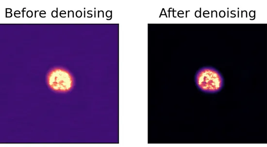
The algorithm has been seen to work on both synthetic and real images, as can be seen, respectively, in figure2.2and in figure2.3.

(44)

Figure 2.3: On the left, a real image before denoising. On the right, the same image after removal of the background. The images have a 1.7× contrast enhancement.

2.5.1 Initial noise

The two curves acquired are reported in figure2.4. The mean difference between the two performances 𝛿(𝑎) = 𝛥_SVD(𝑎) − 𝛥_QR(𝑎)is 0.0 ± 0.2.5 Performing a one-sample Student’s t-test on 𝛿 with null hypothesis that the mean of 𝛿 is 0, we find a T-Statistic value of 1.26, with 98 degrees of freedom, and a corresponding p-value of 0.21: we cannot, therefore, reject the null hypothesis.

We can see that, for small values of 𝑎, we have a large negative value of 𝛥. This is due to the fact that the images of the noise basis, which are subtracted from the image, contain a noisy signal. This, under normal circumstances, is the desired behaviour of the denoising algorithm. However, for small amplitudes of the initial noise, the image will still add some noise, as the weight for a component is found to never be exactly zero. Thus, some noise is added to the image, explaining the sign of the 𝛥. Its magnitude is due to the fact that the initial noise is already very low, and so the added noise can be up to 17 times the initial noise (as can be seen in fig2.4). In denoising done on real images,

(45)

2.5 Results

Figure 2.4: 𝛥as a function of initial noise amplitude, i.e. the parameter 𝑎 in (2.3). In blue, the SVD decomposition, in orange the QR decomposition.

we always found a positive value of 𝛥, and as such we can rest assured that real images always have a sufficient amount of noise for the algorithm to be effective.

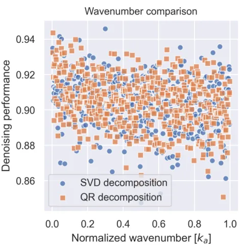
2.5.2 Noise wavenumber

The two datasets acquired are reported in figure 2.5. For the SVD dataset, we have a mean 𝛥_SVD=0.90 ± 1.00, which is identical to the QR one 𝛥_QR.6 _An

(46)

independent sample Student’s t-test, conducted against the null hypothesis that the two distributions have identical means, finds a T-Statistic of 0.13, with 510 degrees of freedom, and a p-value of 0.89. We therefore do not reject the null hypothesis. A linear regression of 𝛥 as a function of 𝑘, suggested by an apparent trend in figure2.5 finds very weak 𝑅2 _{coefficients of 0.05 and 0.07}

for, respectively, the SVD and QR decompositions.

2.5.3 Dimensionality

The two curves acquired are shown in figure2.6; their good overlap suggests a very small difference in performance. The mean value of 𝛿(𝑛) = 𝛥_SVD(𝑛) − 𝛥_QR(𝑛) is (7.081 944 ± 0.000 002) × 10−8, with the standard error taken as uncertainty. A one sample Student’s t-test, against the null hypothesis that this mean value is compatible with 0, results in a t-statistic of 37.8, with 4872 degrees of freedom. The p-value is negligibly different from 0 and we therefore reject the null hypothesis.

We can see that after 10–20 basis components, there is no significant im-provement of the performance. Therefore, a conservative value of 20 elements is adequate for our purposes.

2.5.4 Computation time

The two curves acquired are reported in figure 2.7. As can be seen in the graphs, the QR algorithm is usually faster: 𝑡_QR− 𝑡_SVD is, outside the 29 to 34 component region, between 0.06 s and 0.34 s; however, inside said region, the QR decomposition can be up to 0.97 s slower. At present, we do not have a clear explanation for this quite peculiar behaviour.

2.6 Remarks

The denoising performances of the two algorithm variants are almost identical. Only in one case there has been a statistically significant difference between the two performances: this is probably due to theorem1. Nevertheless, we chose the SVD algorithm, due to its already proven status in this kind of application [38], and the consideration that, for our application, a decomposition which is marginally slower in the average case is preferable to one that is considerably slower in the worst case.

Image enhancement for a Bose-Einstein condensate interferometer

Alma Mater Studiorum · University of Bologna

Image Enhancement for a Bose-Einstein

Condensate Interferometer

Supervisor:

Dr. Francesco Minardi

Submitted by:

Luca Cavicchioli

Sommario

Abstract

Contents

Introduction

1

Theoretical setting

1.1 Atom-light diffraction

1.1.1 Semiclassical atom-light interaction

1.1.2 General theory of the atom beam splitter

1.1.3 Raman-Nath Regime

1.1.4 Bragg regime

1.2 Wave function of a BEC

1.2.1 The Gross-Pitaevskii equation

1.2.2 Interference with BEC

1.2.3 Ideal Bose-Einstein wave function

1.2.4 Interacting Bose-Einstein wave function

1.3 Phase evolution

1.4 Atom interferometry

1.4.1 The Mach-Zehnder and Ramsey interferometers

1.4.2 Measurements with interferometers

2

Background removal algorithm

2.1 Absorption imaging

2.2 The algorithm

2.2.1 Basis calculation

2.2.2 Image projection and noise removal

2.2.3 Denoising performance

2.3 Obtaining the test images

2.3.1 Images of the condensate

2.3.2 Synthetic images

2.4 Decomposition comparisons

2.4.1 Initial noise

2.4.2 Spatial frequency

2.4.3 Dimensionality and computation time

2.5 Results

2.5.1 Initial noise

2.5.2 Noise wavenumber

2.5.3 Dimensionality

2.5.4 Computation time

2.6 Remarks