Automated machine learning : competence development, market analysis and tools evaluation on a business case

POLITECNICO DI MILANO

School of Industrial and Information Engineering

Management Engineering

AUTOMATED MACHINE LEARNING:

COMPETENCE DEVELOPMENT,

MARKET ANALYSIS AND TOOLS

EVALUATION ON A BUSINESS CASE

Supervisor: Prof. Barbara Pernici

Correlator: Alessandro Volpe

Master Degree by:

Tommaso Curotti 905582

Abstract

Today data are increasing in volume and in complexity every day, to follow this exponential growth are necessary new methods to analyze the enormous amount of data generated. Companies have understood that data are essential to compete, and they are collecting even more data, but sometime happens that they do not have the resources to analyze them. The actual problem is not how to generate data but how to analyze data. The real problem today for companies is the scarcity of expert data scientists able to extract value from Big Data. To solve this problem are arising new technologies of data management and analysis. One of the most potential innovation in this field is the automated machine learning. The thesis aims to define it considering different perspectives to increase knowledge and to test how these systems work.

Automated machine learning is the new technology enabling the development of machine learning models autonomously by the machine. These systems reduce the level of interaction human-machine, letting the machine to decide how to create complex models to solve complex problems. Machine learning is in the hand of few skilled people, data scientists, having deep knowledge in computer science, mathematics and statistics. With AutoML systems this equilibrium is wrecked since even persons without strong skills can rapidly develop machine learning solutions.

To create a comprehensive ‘big picture’ of this world, different analysis both qualitative and quantitative were executed. Qualitative researches were carried about understanding what automated machine learning is, researching the reasons why this new technology is becoming even more requested by companies and studying the potential impact that it could bring to data science professional figures in doing their jobs. Quantitative analysis was about both quantification and classification of the actual AutoML systems, trying to define the number of different solutions in existence today and their target customers. Always regarding the quantitative researches were tested different automated machine learning systems, precisely five, comparing their performances with those one of two different machine learning solutions really implemented to solve a prediction problem for a gas dispatching company. The comparison was conducted considering a specific trade-off composed by three main drivers: MAPE as metric to establish the goodness of the different models compared; the economic return, directly correlated to MAPE, brought by the different solutions in order to understand if AutoML can achieve the same results obtained by traditional machine learning; the set of time, cost and effort needed to develop the different model of prediction both for AutoML and traditional machine learning. This final part of the thesis aims to answer to the question: could AutoML be considered as a valid alternative to traditional machine learning workflow? As will be seen from the conclusions drawn from the tests carried out on the business case under consideration, this new technology drastically reduces development time and costs, but does not always respect the level of performance desired. The choice whether to adopt these systems or not is based on the triple trade-off performance-time-development costs.

Abstract (italiano)

Ogni giorno i dati stanno aumentando di volume e complessità, per seguire questa crescita esponenziale sono necessari nuovi metodi per analizzare l'enorme quantità di dati generati. Le aziende hanno capito l’importanza dei dati per competere nel mercato e per questo stanno aumentando la quantità di dati raccolti, ma capita che sempre più spesso non dispongono delle risorse per analizzarli. In effetti, oggi il problema non è come generare dati ma come analizzare i dati. Il problema per le aziende oggi è la scarsità di esperti data scientist capaci di estrarre valore dai Big Data. Per risolvere questo problema stanno nascendo nuove tecnologie di gestione e analisi dei dati. Una delle innovazioni col più grande potenziale in questo campo è il machine learning automatizzato. La tesi mira a definire questa tecnologia considerando diverse prospettive per aumentare la conoscenza su di essa e testare come effettivamente questi sistemi performano.

Il machine learning automatizzato è una nuova tecnologia che permette alla macchina di sviluppare autonomamente modelli di machine learning. Questi nuovi sistemi riducono il livello di interazione uomo-macchina, permettendo alla macchina di decidere come creare un modello di machine learning per risolvere problemi complessi. Il machine learning è nelle mani di poche persone, i data scientist, i quali hanno profonde conoscenze in computer science, matematica e statistica. Con i sistemi di AutoML questo equilibrio potrebbe vacillare, dato che anche persone senza forti competenze possono rapidamente sviluppare soluzioni di machine learning.

Per creare una comprensiva ‘big picture’ di questa tecnologia sono state eseguite diverse analisi sia qualitative che quantitative. Le ricerche qualitative sono focalizzate nel definire il machine learning automatizzato, ricercando le ragioni del perché questa nuova tecnologia stia diventando sempre più richiesta dalle aziende. Inoltre, è stato oggetto di ricerca indagare sul potenziale impatto che l’AutoML potrebbe portare nel metodo di lavoro dei data scientist durante il tipico processo di sviluppo di un modello di machine learning. Le analisi quantitative, invece, sono state condotte al fine di classificare e quantificare i sistemi AutoML presenti oggi nel mercato e per definire quale sia la loro strategia di targeting.

Sempre riguardo le ricerche quantitative sono stati testati diversi sistemi di machine learning automatizzato, precisamente cinque, comparando le loro performance con quelle di due soluzioni di machine learning tradizionale realmente implementati per risolvere un problema di previsione per una compagnia che si occupa di dispacciamento di gas. La comparazione è stata fatta considerando uno specifico trade-off composto da tre driver principali: il MAPE come metrica per definire la bontà dei diversi modelli confrontati; il ritorno economico, direttamente correlato al MAPE, portato dalle diverse soluzioni per capire se l’AutoML può ottenere gli stessi risultati ottenuti dal machine learning tradizionale; l’insieme di tempo, costi e sforzo necessario per sviluppare i diversi modelli di previsione sia delle soluzioni automatiche che di quelle tradizionali. Questa parte finale della tesi cerca di rispondere alla domanda: l’AutoML potrebbe essere una valida alternativa al tradizionale metodo di lavoro per sviluppare modelli di machine learning? Come si evincerà dalle conclusioni tratte dai test effettuati sul business case preso in considerazione, questa nuova tecnologia riduce drasticamente il tempo e i costi di sviluppo, ma non sempre rispetta il livello di performance voluto. La scelta se adottare questi sistemi o meno è basata sul triplice trade-off performance-tempo-costi di sviluppo.

Table of Contents

1.3 Machine Learning Introduction ... 16

1.4 Machine Learning Pipeline ... 20

1.4.1 Data Cleaning ... 22 1.4.2 Feature Engineering ... 24 1.4.3 Feature selection ... 28 1.4.4 Model selection ... 30 1.4.5 Hyper-parameters optimization ... 33 1.4.6 Model evaluation ... 35

1.5 Machine Learning problems ... 40

1.6 Automated Machine Learning ... 42

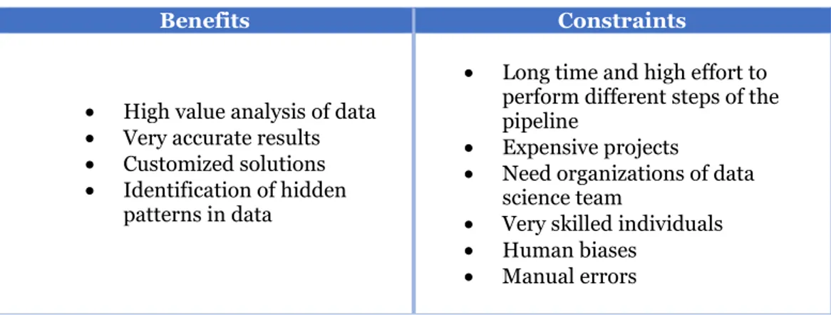
1.7 AutoML Benefits and Constraints ... 44

2 Impact on Data science ... 46

2.1 CRISP-DM model with AutoML ... 47

2.2 Deep-dive on Data Scientist ... 49

2.3 New professional role: Citizen Data Scientist ... 53

3 AutoML Market Analysis, Innovation and Benchmarking ... 57

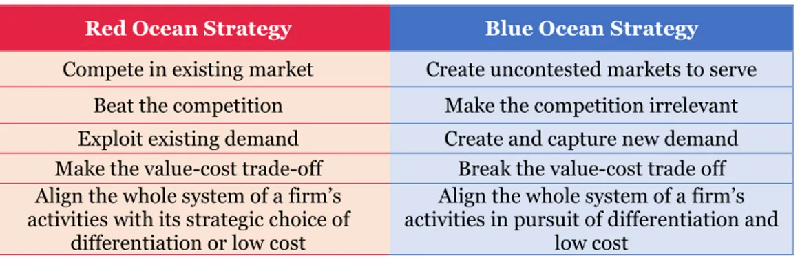
3.1 AutoML: Innovation & Strategy ... 58

3.2 AutoML: Market Pull ... 61

3.3 AutoML Market Research: Methodology ... 63

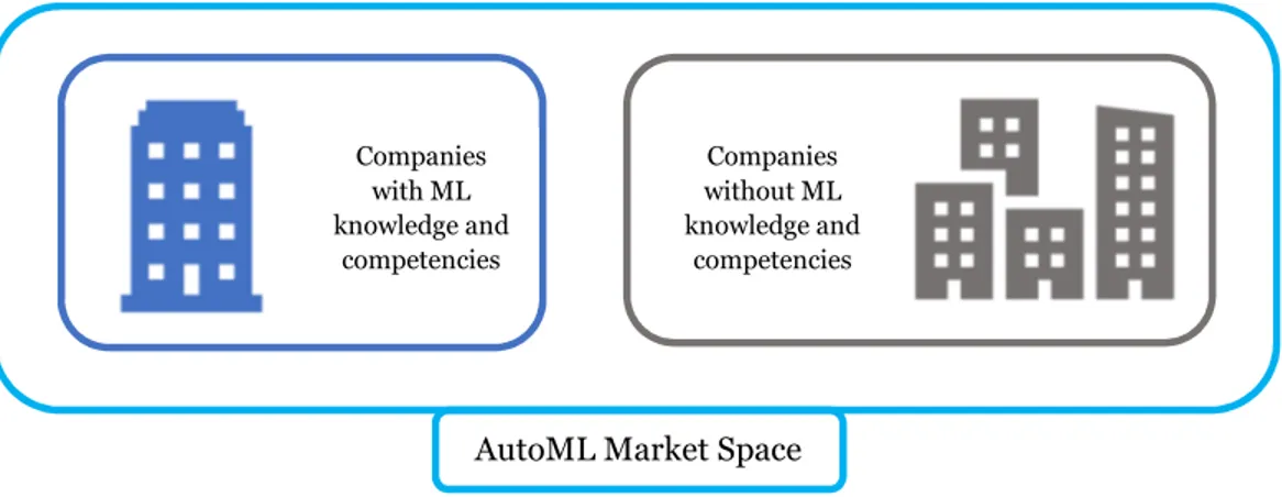
3.4 Market Big Picture ... 66

3.5 AutoML Customers Analysis ... 71

3.6 Deep-dive on AutoML tools used in business case ... 79

4 business case: a comparison between automl and ml models ... 85

4.1 Business context ... 87

4.3 Situation before Bip ... 92

4.4 Bip first solution: ANN ... 93

4.5Bip second solution: Ensemble ... 98

4.6AutoML experiments ... 102

4.6.1Google Cloud AutoML Tables ... 105

4.6.2Dataiku ... 108 4.6.3Azure ML Microsoft ... 113 4.6.4H2O Driverless AI ... 115 4.6.5 AWS Sagemaker ... 116 4.7 Final insights ... 117 5 Conclusions ... 121

5.1 Future researches and applications ... 124

Bibliography ...125

Webography ... 127

LIST OF TABLES

Table 1 - Differences between traditional statistics and ML ... 17

Table 2 - Example of binning technique, on the right for numerical features and on the left for categorical features ... 26

Table 3 - Example of one-hot encoding ... 27

Table 4 - Confusion Matrix ... 36

Table 5 - Benefits and constraints of ML ... 41

Table 6 - AutoML benefits ... 44

Table 7 - AutoML constraints ... 45

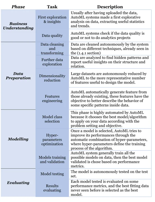
Table 8 - Phases automated by AutoML systems ... 48

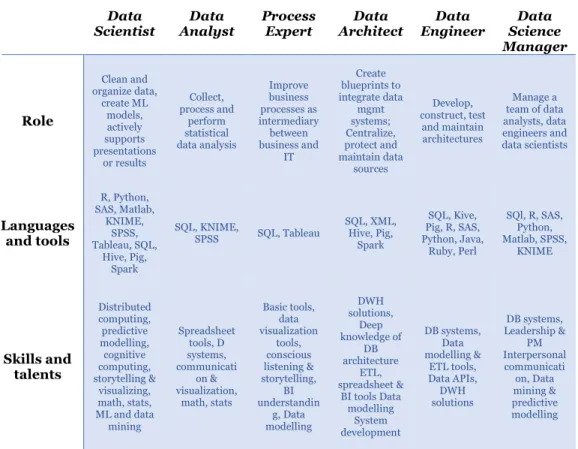
Table 9 - Data Science professional roles ... 50

Table 10 - Differences between a blue ocean and a red ocean strategy ... 59

Table 11 - AutoML tools classification framework ... 63

Table 12 - Table listing all the AutoML tools considered in the market analysis ... 67

Table 13 - Table listing all the AutoML customers, regarding the tools analyzed in the market analysis ... 72

Table 14 - Principles of the resolution ... 88

Table 15 - Table listing the three performances instituted by the authority ... 89

Table 16 - Input data ... 92

Table 17 - ANN main characteristics ... 94

Table 18 - Table defining the data used to build all the six models ... 98

Table 19 - Ensemble main characteristics ... 99

Table 20 - Economic results between the three solutions in different periods of time .. 101

Table 21 - Characteristics of each dataset used in business case ... 103

Table 22 - Three different target with tree different timeframe structures ... 103

Table 23 - Performances obtained using Google AutoML Tables ... 105

Table 24 - MAPE and incentives obtained by the different models built by GCP ... 107

Table 25 - Time periods of the successive tests conducted with Dataiku ... 108

Table 26 - Performances obtained using Dataiku ... 108

Table 27 - MAPE and incentives obtained by the different models built by Dataiku ... 110

Table 28 - Performances obtained by Dataiku on further tests made on 2/2018 and 6/2018 ... 111

Table 29 - MAPE and incentives obtained by the different models built by Dataiku on further target periods ... 111

Table 30 - Performances obtained using Azure ... 113

Table 31 - MAPE and incentives obtained by the different models built by Azure ... 114

Table 33 - MAPE and incentives obtained by the different models built by H2O Driverless AI ... 115 Table 34 - Performances obtained using AWS Sagemaker... 116 Table 35 - MAPE and incentives obtained by the model developed by AWS Sagemaker ... 116 Table 36 - Full comparison between AutoML solutions and ML solutions (ANN and Ensemble) ... 117 Table 37 - Comparison of 3 drivers: Time, Full Time Employee and Cost related to each solution ... 119 Table 38 - Benefits and constraints emerged from the tests conducted on AutoML with our specific problem ... 120

LIST OF FIGURES

Figure 1 - 5 V of Big Data ...13

Figure 2 - How machine learning works... 16

Figure 3 - Work-flow of statistical model development ... 17

Figure 4 - Work-flow of ML model development ... 17

Figure 5 - Machine Learning algorithms ... 18

Figure 6 - CRISP-DM Model ... 20

Figure 7 - First preprocessing step ... 22

Figure 8 - Data cleaning main techniques ... 22

Figure 9 - Feature engineering steps ... 24

Figure 10 - Main feature engineering techniques ... 25

Figure 11 - Example of log transformation ... 26

Figure 12 - Feature selection techniques ... 29

Figure 13 - Overfitting, blue line ... 30

Figure 14 - Underfitting, red line ... 30

Figure 15 - Dataset splitting methods: train and test ...31

Figure 16 - Model selection techniques ...31

Figure 17 - Cross validation technique ... 32

Figure 18 - Early stopping technique ... 32

Figure 19 - Hyper-parameters optimization techniques ... 34

Figure 20 - Grid and Random search ... 34

Figure 21 - ROC curve ... 37

Figure 22 - AUC ... 37

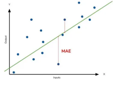
Figure 23 - MAE ... 38

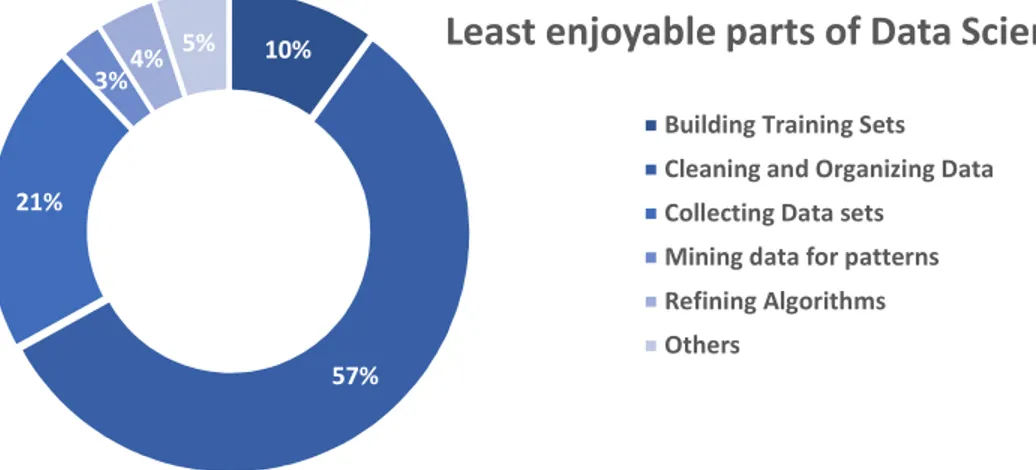
Figure 24 - Results of the survey made by Forbes ... 40

Figure 25 - Graphical pipeline with and without AutoML ... 43

Figure 26 - Functions automated by AutoML considering the CRISP-DM model ... 47

Figure 27 - Citizen data scientist profile ... 53

Figure 28 - Google cloud AutoML service diversification ... 60

Figure 29 - Blue Ocean strategy of AutoML ... 60

Figure 30 - Innovation model to define a new technology ... 61

Figure 31 - AutoML classification map ... 65

Figure 32 - Market analysis framework ... 66

Figure 33 - Cumulate of AutoML tools products per year ... 69

Figure 34 - Map highlighting the countries in which AutoML system considered in the market analysis have been developed ... 70

Figure 36 - Count of AutoML customers per industry ... 76

Figure 37 - Pie chart to highlight the classes of AutoML customers considering their size ... 77

Figure 38 - Bar chart highlighting the average size of the customers per AutoML tool .. 78

Figure 39 - Framework developed to analyze in depth an AutoML tool ... 79

Figure 40 - Evolution of ML models to predict the gas day-ahead ... 86

Figure 41 - Four main processes of gas dispatching ... 87

Figure 42 - Legislation structure ... 88

Figure 43 - Incentives structure, relation between MAPE and Incentive... 89

Figure 44 - ARIMA model input and output ... 90

Figure 45 - Data input in ANN ... 93

Figure 46 - Comparison between ANN and ARIMA, in simulation ... 94

Figure 47 - Incentives comparison between ANN and ARIMA in simulation... 95

Figure 48 - MAPE comparison between ANN and ARIMA in production ... 96

Figure 49 - Incentives comparison between ANN and ARIMA in production ... 96

Figure 50 - Histogram figuring the MAPE for each month achieved by ANN, in blue the yearly MAPE ... 97

Figure 51 - Data input in Ensemble ... 98

Figure 52 - MAPE comparison between Ensemble and ANN in simulation ... 99

Figure 53 - Incentives comparison between Ensemble and ANN in production ... 100

Figure 54 - AutoML tools used for the business case, from left to right: Google AutoML Tables, Dataiku, Azure, AWS Sagemaker, and H2O Driverless AI ... 102

Figure 55 - Temporal split between training datasets and test datasets, considering 10/2017 as the test set ... 103

Figure 56 - Excel page showing the steps to calculate the incentives gained or lost... 106

Figure 57 - Incentives during October 2017 considering the model built on the raw dataset (the best obtained by Google) ... 106

Figure 58 - Excel page showing the steps to calculate the incentives gained or lost ... 109

Figure 59 - Incentives during October 2017 considering the best model with MAPE of 4,53% ... 110

Figure 60 - Azure workflow ... 113

Figure 61 - Overall performances obtained by each tool for every model developed, comparing MAPE of every model with the two thresholds given by the monthly MAPE of ANN and by the monthly MAPE of Ensemble ... 118

Figure 62 - Comparison between incentives gained or payed adopting AutoML or ML in October 2017 ... 119

Figure 63 - Trade-off ... 120

1 INTRODUCTION

In recent years the world has seen an exponential growth of machine learning (ML) techniques in many fields and industries. However, ML methods are very sensitive to a wide range of variables and design decisions, which are a considerable barrier to new users of these techniques. ML can be split into many subdivisions covering a very large territory of knowledge and competencies, which need deep knowledge in many fields. To simplify the adoption of ML was born the automated machine learning (AutoML) that aims to automate the entire pipeline from data preprocessing to model selection. AutoML is the core topic of this thesis. It is a very new hot topic in the field of Artificial Intelligence (AI) that could bring massive changes in the various methods companies and professionals work with data and develop high-value ML models. The idea behind AutoML is to automate ML pipelines, where pipelines are all the sequence of steps that a traditional project of ML has to pass through to achieve its results. Ideally, AutoML is an extremely powerful tool that enables everyone to conduct analysis and project on data even without knowledge in programming, mathematics, and statistics. AutoML can lead to improved performance of the models while reducing the time and effort spent by data scientists. As consequence, AutoML gained a real commercial value in recent years and several big companies are developing their AutoML systems to sell in the market. The purpose of democratizing ML is not to impute only to proprietary tools but also to open source tools, both deep analyzed in the chapter of the market analysis.

In the following chapters we will go through different aspect of AutoML, trying to describe how it works and what it is changing in the field of ML, then the impact that it has on the market, organization, professional role and to conclude we will analyze all these aspects in a very insightful business case developed in Bip. xTech. The business case will show the differences between a predictive ML project for an oil & gas company and then it will compare the same project developed with five different proprietary AutoML tools tested in Bip, to build a useful benchmark and point out the benefits and the constraints that AutoML has over ML. The tools used to develop the business case are Google Cloud AutoML Tables, Dataiku, Azure ML Microsoft, AWS Sagemaker and H2O Driverless AI.

1.1 Objectives

Being AutoML very new there are few types of research about it and a difficult part of this thesis was to define its objectives. The difficulty was given by the type of analysis to conduct: the indecision was about to develop a technical thesis covering the technicalities behind the implementation and construction of an AutoML system or to highlight AutoML impact in the market, in the organization, on the performance, and professional data science roles. Thus, we decide to make an inside-out analysis that tries to describe and build an overview of what an AutoML system can do and then go to analyze the impact that it has on the external variables. So, to build an inside-out analysis we defined four principal objectives to achieve:

1. To create knowledge and awareness about a very new hot topic in the field of data science, automated ML. The research is not aimed to describe in detail the technicalities and algorithms behind the AutoML solutions, but to point out the main characteristics of these new tools and to explain which part of the traditional ML pipeline AutoML impacts.

2. To understand how AutoML is changing the world of data science, in this perspective the focus will go on the study of three main impacts:

• Data scientist profession

• Arising professional role: the citizen data scientist

• Organization of data science workflow, considering the CRISP/DM model

3. To create the big picture of the actual tools both proprietary and open source based on some features selected to classify these tools. After having created the big picture of the actual market we will analyze the main customer base of the most important proprietary tools to understand which kind of industries are interested and are using AutoML solutions. This chapter will be concluded with a deep-dive on the tools used in the business case of the fourth chapter.

4. To show what are the differences between a traditional ML project and the same project develop with different proprietary AutoML tools. This part will be integrated and explained with a real case developed in Bip.xTech. The Business case will be structured as follow:

• Description of the context in which the oil & gas company operates

• First intervention of Bip and results

• The second intervention of Bip and results

• Description of the same project developed with AutoML tools

• Comparison of the different solutions

• Conclusions

The whole thesis is focused to achieve the first objective: to create knowledge and awareness about all what concerns this new field under different point of views. Instead for the other three objectives, there is a dedicated chapter that treats a specific argument. To achieve these four objectives the thesis will begin from the history of ML and why it is fundamental to deal with data. Then we will introduce the new branch of artificial

intelligence called AutoML. Introducing AutoML we will focus our attention on the birth of AutoML and then we will go in-depth about how it impacts the traditional ML pipeline, discovering what are the main functionalities, benefits, and constraints that AutoML brings with itself, firstly from a theoretical point of view and then from a practical perspective adopted in the Chapter 4 where we will analyze AutoML experiments. Once we concluded the introduction part the focus will go towards the second section of the thesis that tries to satisfy the objective of understanding the impact that AutoML has on the professional role of data scientists and on the organization of the data science team. Since that, theoretically, AutoML can perform all the tasks that usually are executed by data scientists, it is interesting to discuss the possible future scenarios in data science and to describe the new role emerging thanks to AutoML. This part will be integrated with some important professional article analysis (Forbes, Forrester, and Gartner).

The third part of the thesis, treating the relative objective, is aimed to create a benchmark of the different tools. To build a concrete big picture of what kind of solutions we can find in the market today, we will discuss and analyze through a consistent market analysis all the available tools in the market nowadays. In order to comprehend that it is not just a theoretical topic but a real added-value for every company that deals with Big Data, during the market analysis, the major information that we will extract will be the typology of the different tools (open source or proprietary), who are the leaders of the market and all the technical functionalities of each tool analyzed. An insightful part of the market analysis aims even to map and classify the target customers for the main proprietary tools for which are available trustable information about their customers with relative business cases published on their websites.

The final part, aimed to satisfy the fourth objective of the thesis, is a practical comparison between traditional ML projects developed in Bip.xTech, a very successful case of study, and the same problem solved through the usage of different AutoML tools.

The different solutions will be analyzed under three main key performance indicators (KPI):

• MAPE (Mean Absolute Percentage Error)

• Economic return (potential incentive gained or lost)

• Project cost, time and effort

This comparison is very useful to comprehend in which measure AutoML can help companies and data scientists to do ML projects. All the details will be discussed in Chapter 4.

1.2 Big Data

Before starting to talk about automated ML is important understand why society, companies, people and everything is around us need to deal and comprehend a very important element: data. The main reason could be imputed to Internet. Internet is the reason of the technological evolution that lead humankind to develop new ways to deal with things around us, adopting new ways to communicate, to interact, to move and to behave.

So, in order to understand why we talk about automated ML we can start from Big Data that is one of the main consequences of Internet growth and enabling devices diffusion.

“Big data usually includes data sets with sizes beyond the ability of commonly used software tools to capture, curate, manage, and

process data within a tolerable elapsed time.” [1] From the definition, Big Data are very huge amount of data that can’t be analyzed with common tools because the time needed is too long and today actions must be taken faster. Big data usually includes data sets with sizes beyond the ability of commonly used software tools to capture, curate, manage, and process data within a tolerable elapsed time. Big Data are created by every single person or device connected through Internet or able to collect and store data. Big Data are all those data on which is possible to conduct analysis trying to extract important information, they have a real value if managed efficiently. Usually, to define Big Data is used the 5 Vs model that explain the concept of Big Data with its 5 main characteristics:

Velocity: obviously, velocity refers to the speed at which vast amounts of data are being generated, collected and analyzed. Every day the number of emails, twitter messages, photos, video clips, etc. increases. Every second of every day data is increasing. Increasing the velocity of data generation means also increasing of the pace at which they are generated. This leads us to develop new method to handle this new dynamic situation.

Variety: variety is defined as the different types of data we can now use. Data today looks very different than data from the past. We no longer just have structured data (name, phone number, address, financials, etc) that fits nice and neatly into a data table. Today’s data is unstructured. In fact, the Computer World magazine states that unstructured information might account for more than 70%-80% of all data in organizations. New and innovative big data technology is now allowing structured and unstructured data to be harvested, stored, and used simultaneously.

Variability: the meaning or interpretation of the same data may vary depending by the contest in which it is collected and analyzed. The value, thus, is not held by the data itself but it is strictly linked to the contest to which come from.

Volume: it refers to the incredible amounts of data generated each second from social media, cell phones, cars, credit cards, M2M sensors, photographs, video, etc. The vast amounts of data have become so large in fact that we can no longer store and analyze data using traditional database technology.

Value: it refers to the real value of the Big Data, they record significant events with several types of data correlated from each other. From the analysis of these data is possible understand why events happens and which are the important factors related to events. Veracity: Veracity is the quality or trustworthiness of the data. It is the degree to which data is accurate, precise and trusted [2].

Big Data comprehend all kind of data, but when we deal with data analysis or data projects is fundamental to comprehend what kind of data we are treating. It is fundamental to define the type of data because consequently, based on the type of data there will be a specific set of activities and task to perform on them. Typically, data are segmented in 3 main sets:

• Structured Data: they are data collected with a clear organization, usually with a tabular form where each event has different features characterizing it. Considering a table each row represents an event and each event has its own features that correspond to the number of columns.

• Unstructured Data: they are data collected without an organization, they are not clear and extracting information from them is very difficult because they are not pre-defined in a clear manner. When we talk about unstructured data, we refer to images, videos, records and so on.

• Semi-structured Data: they are data that belong to structured data but do not obey to formal structure, they may be not collected in a tabular form and they may not have all the same features.

Every day, every hour, every minute and every second many data are created by people, machine, companies, application and everything is digital and has the capability to record events and consequently data. In the last year we are seeing an increase of data generation due to the availability of interconnected devices to Internet, new software and cheaper solution to collect and store data.

A real impressive fact is that the 90% of the existing data were create only in the past 2 years [3]. Data are growing exponentially, and this is the reason why they are getting importance and value now, because before there were not so many data to extract

information and patterns useful to conduct business decisions. As we can deduct from this situation, and how we can see from the market, nowadays the top-companies in the world are those ones that are able to use and extract very important information from data they create and gathered.

Big Data doesn’t mean new hardware or software, it means new way of looking at data, new extended information outside the company and new type of analysis. To extract value from Big Data, we need analytical models. To create analytical models, we require a team of data scientists.

This rapid evolution of businesses, data creation and collection led to create a new method to manage and to leverage on data named Machine Learning, a method to deal with Big Data that enables computers to learn from data patterns and to develop models able to extract value from data with the supervision of high-skilled professionals, called data scientists. This professional figure will be the focus of the following Chapter 2.

1.3 Machine Learning Introduction

“Machine Learning (ML) is the scientific study of algorithms and statistical models that computer systems use to perform a specific

task without using explicit instructions, relying on patterns and inference instead. It is seen as a subset of artificial intelligence (AI).

ML algorithms build a mathematical model based on sample data, known as "training data", in order to make predictions or decisions

without being explicitly programmed to perform the task.” [4]

Figure 2 - How machine learning works

ML idea is to enable machines to learn how to behave from past data, allowing them to take actions or make predictions with a minimum human intervention. ML is characterized by different methodologies, techniques and tools on which perform its capabilities. It is possible to say that when we are talking about ML, we are intending different mechanisms that allow to an intelligent machine to improve its capabilities and performances during time.

At the base of ML there are a set of different algorithms that will be able to take one decision instead of another, or able to execute actions learned in the past. Before the birth of ML, the highest level of data analysis is what we call traditional statistics. To understand the changes brought by ML techniques is useful have a picture of what were the characteristics before and then ML:

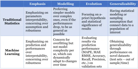
Table 1 - Differences between traditional statistics and ML

Emphasis Modelling Evolution Generalizability

Traditional Statistics Emphasizing on parameters interpretability, concerning over assumption and robustness Preferring simpler models over complex ones, even if the performances drop, to be as general as possible Focusing on a-priori hypothesis and statistical significance of results Having statistical modeling or sampling assumption that connect data to a population of interest Machine Learning Emphasizing on prediction and performances over interpretability, concerning over robustness Concern for overfitting but not model complexity per se, which can dynamically adapt to changes over time Evaluating results via prediction performance (MAPE, MAE RMSE, Accuracy, Recall, Precision, etc..) on validation sets Obtaining generalizability through performance on novel datasets (test sets – out of sample/time)

The two different solutions can be easily shaped with the two following schemes. Traditional Statistics Machine Learning Input Rules Statistical Models _Output Input Output ML Models Learn Rules New Input ML Models Predict Output Figure 3 - Work-flow of statistical model development

The big difference that we can immediately see is the conceptual method to approach the problem. If with the traditional statistics the objective is to find patterns inside data thanks to mathematics knowledge, with ML the objective is to allow machine to learn patterns from training data and then to apply these patterns (models) to new data never seen to make predictions or classification tasks. Statistics is at the base of ML but with a narrow purpose: analyze known data. Instead ML wide the purpose and tries to get accurate predictions thanks to the analysis of past data.

The algorithms of ML are different from each other for their approach to the problem, for the type of data input and output and the type of task or problem they are trying to solve. The algorithms can be divided as follow:

Figure 5 – Machine Learning algorithms Supervised Learning

In this case, these algorithms build a mathematical model based on a set of data that contains both the inputs and the desired outputs. The data on which the model is build is called training data, and it is a dataset of records used to train the model. Supervised learning algorithms after the training phase are able to predict with high accuracy (it depends on the goodness of the model) the output of a new input set. Such algorithms are considered good when they are able to correctly determine the output for inputs that it has never seen before.

These algorithms could be both of classification or regression:

• Classification Algorithms: they are used when the output belongs to a restricted set of values.

• Regression Algorithms: they are used when the output may have any numerical value within a range.

Machine Learning

Algorithms

Supervised

Algorithms

Classification

Algorithms

Regression

Algorithms

Unsupervised

Algorithms

Clustering

Algorithms

Semi-supervised

Algorithms

Reinforcement

Algorithms

Semi-supervised learning

It is similar supervised learning algorithms but in input data miss some outputs. The goal of a semi-supervised model is to classify some of the unlabeled data using the labeled information set.

Unsupervised Learning

In this case the algorithm takes a set of data in which are included just the inputs without any output. The algorithm has the task to find hidden patterns and structures in data that explain how data are correlated. The algorithm learns from input data that has not been labeled, categorized or classified. The most famous example is the cluster analysis on a dataset:

• Clustering Algorithms: they try to divide the observations of a dataset in subsets also called clusters, based on similarity or other predefined criteria. Consequently, if observations inside one cluster are similar, observations inside different clusters are dissimilar.

Reinforcement Learning

It is a branch of ML that is concerned with the computer programs or also called software agents, enable them take actions in an environment so as to maximize some notion of cumulative reward. It differs from supervised learning in that labelled input/output pairs need not be presented, and sub-optimal actions need not be explicitly corrected. Instead the focus is finding a balance between exploration and exploitation [5].

1.4 Machine Learning Pipeline

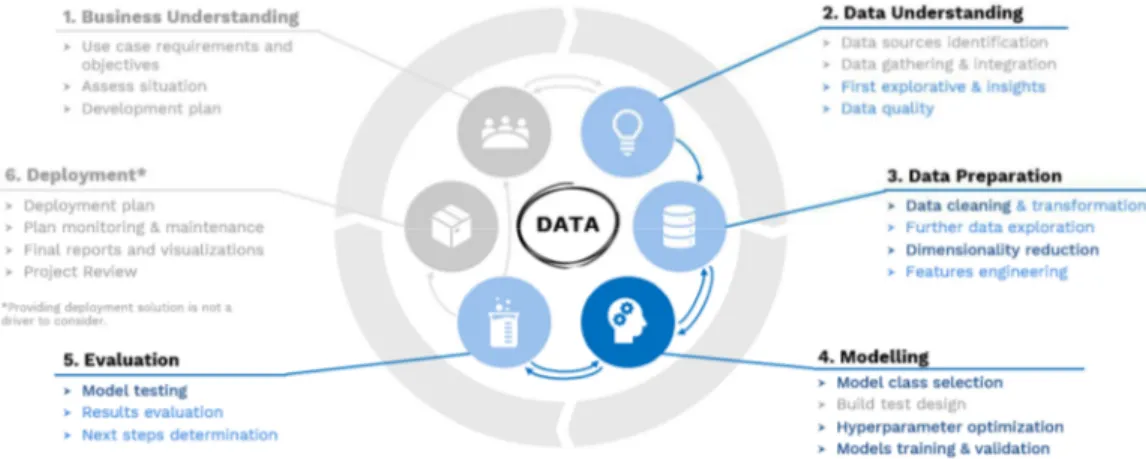
A model that describe the organization of a ML project is the CRISP-DM framework. CRISP-DM stands for Cross-Industry Standard Process for Data Mining. It gives a structured planning even for a ML project. This model explains the state-of-the-art of a model development. In practice many of the tasks can be performed in a different order and it will often be necessary to backtrack to previous tasks and repeat certain actions. The framework is composed by the following points:

1. Business understanding

The first stage of the CRISP-DM framework is to understand the business objectives, uncover the hidden factors that could lead the project to better results. In order to define the right objectives to achieve is mandatory to assess the actual situation and then to develop a plan of actions.

2. Data understanding

The second stage of the model is centered on the data sources of the project. The important data must be identified, gathered and integrated. After having all important data is useful to do a first explorative analysis on them to extract some insights. Another important task to be done is to check the quality of data.

3. Data preparation

This objective of this stage is to prepare data before creating the ML model. Data to ingest in the model must be very relevant, data before being considered good has to pass different stage, they must be cleaned and transformed, they must be analyzed deeper to detect some important information. If only some data are relevant is necessary to apply some dimensionality reduction methods. If needed data can be created through some feature engineering techniques.

4. Modeling

The fourth phase of CRISP-DM model is the modeling, in this phase data scientists must select the ML model to apply and tune the hyper-parameters to improve model training. Once a model is trained it must be evaluated according some metrics chose to describe meaningfully the ability of the model.

5. Evaluation

Once a model is trained it must be evaluated according some metrics chose to describe meaningfully the ability of the model. This phase is characterized by tests applied to the model in order to understand if it fit well unknown situation.

6. Deployment

The last phase of the model is the implementation of the model, with the creation of a monitoring system to collect the results and keep the model always update if something goes wrong.

This model gives an overview of a traditional ML project, the next section will give you a deeper description of the different techniques involved in all the steps. Now that we have a general idea about the different tasks that a ML project must deal with, we can introduce some technical aspects to embrace when dealing with ML. A model, or better the model development, is the core activity of every ML project. The model is the logical structure developed to deal with specific data, aiming to obtain the expected output also from data never seen before. A model is a mathematical representation of a real-world process, it is derived from the training set by which the ML algorithm learn from. Creating a model is in general is a very complicated task, there are a lot of problems to manage and many steps to solve. Let’s go to see the most famous and used techniques during the pipeline: the pipeline is the sequence of steps needed to build a consistent ML model.

The sequence of steps is not linear but iterative until the model is not good enough, as we have seen from the CRISP_DM organization could be present many backtrack between phases until the performance is not achieved. In each step the data are modified and transformed from a raw to a clean and understandable situation, depending on the algorithm to apply on the data.

Now let’s go deeper in detail within each phase to understand the essential activities to perform on data. The objective of the following six subsections about the ML pipeline is to define the traditional activities performed during a project. The explanation of the main techniques involve in ML is useful to understand and to highlight the complexity involved behind an AutoML solution that typically works with a friendly drag and drop interface or with few steps where no code is necessary.

1.4.1 Data Cleaning

Once you have collected the raw data (raw data means data picked and collected by a source, they are set of data uncleaned and with possible errors and inconsistences), to become valuable for ML activities those data must be cleaned by the outliers, by the null values and so on. The first data preprocessing step of a ML pipeline is to clean your data.

We must know that data cleaning techniques vary from dataset to dataset based on the configuration of data and on the objectives of the analysis. Proper data cleaning can make or threat your project, it is a very important phase. Usually professional data scientists spend a very large portion of their time to complete in the better way possible this step. Why is it so important? For two reasons well explained by the following two cites:

1. “Garbage in is garbage out” [6]

It means that if you build a ML model on bad data, even the model will result bad and the output won’t be accurate as you want.

2. “Better data beats fancier algorithms” [7]

It means that it is better having a good dataset cleaned and preprocessed than a very good algorithm, the cause is that ML model are built on the data they are analyzing and the better they are the better will be the model.

Basically, both the “laws” say that in order to obtain a very good model, the first action to do is to transform skewed, raw and noisy data in a clean form suitable for algorithms to extract values from them.

The main methods to clean data are the following:

Figure 8 - Data cleaning main techniques

Data Cleaning

Techniques

Remove

unwanted

observations

Fix structural

errors

Filter unwanted

outliers

Handle missing

values

Raw Data _{Data Cleaning Techniques} Clean Data

1. Remove unwanted observations, this includes duplicate or irrelevant observations.

2. Fix structural errors, these errors arise during measurement, data transfer, or other types of “poor housekeeping”.

3. Filter unwanted outliers, they can cause problems with some models, but they are innocent until proven guilty, only if you have a legitimate reason to remove an outlier, it will help your model’s performance.

4. Handle missing data, it is a deceptively tricky issue in applied ML because you can’t just ignore them in your dataset since that many algorithms do not accept missing values. The two most commonly methods to handle missing values are dropping observations that have missing values or imputing the missing values based on other observations, but these two methods are not considered the more intelligent. Typically, you can have to deal with numerical of categorical missing values in a dataset and for each of them there are different techniques. With specific class of data as categorical ones, you can simply label them as “Missing”, simply you are adding a new class and the algorithms can handle it. For Numeric data you should flag and fill the values, that means flag an observation with an indicator carriable of missingness and then fill the original missing value with 0 just to meet the technical requirement of no missing values.

The final objective of this phase is to have a high data-quality to feed the ML algorithms, high-quality data must pass a set of criteria to be considered ‘good’.

• Validity: the degree to which the measures conform to defined business rules or constraints.

• Accuracy: the degree of conformity of a measure to a standard or a true value. It is very hard to achieve through data-cleansing in the general case, because it requires accessing an external source of data that contains the true value; such “gold standard” data is often unavailable.

• Completeness: the degree to which all required measures are known. Incompleteness is almost impossible to fix with data cleansing methodology: one cannot infer facts that were not captured when the data in question was initially recorded.

• Consistency: the degree to which a set of measures are equivalent in across systems. Inconsistency occurs when two data items in a dataset contradict each other. Fixing consistency is not always possible.

• Uniformity: the degree to which a set of data measures are specified using the same units of measure in all systems.

Once you are sure to have cleaned and made consistent your dataset, satisfying the precedent criteria, you can start building your ML algorithms.

We can notice that this part in the traditional way is very long and there are a lot of variables to consider. Usually this phase takes long time to be executed by data scientists. The next phase of the pipeline is a set of activities intercorrelated, it is the feature engineering phase.

1.4.2 Feature Engineering

It is the process in which typically data scientists use their domain knowledge of the data to create features that allow the best application of ML algorithms. It is a fundamental phase of ML, and it is both difficult and expensive in time and effort. The objective of this phase is to create and select the best set of features to build the model.

“Coming up with features is difficult, time-consuming, requires expert knowledge. ‘Applied machine learning’ is basically feature

engineering.” (Andrew Ng, Stanford University)

A feature is an attribute or property shared by all the independent units on which analysis or prediction is to be done. Any attribute could be a feature, until it is useful to the model. The purpose of features, other than being attributes, would be much easier to understand in the context of a problem. Feature are important for predictive models because they influence the results that you are going to achieve with the model selected. The quality and quantity of the features will have great impacts on whether the model is good or bad. (in our business case in Chapter 4 will be faced a predictive problem solved with different models built on datasets with different set of features, with the objective to understand how the results rely on features in input.

Choose the right features is very important because better features can create simpler and more flexible models, and they often yield better results.

The typical process of feature engineering is composed as follow:

Brainstorming

Deciding what features to create

Creating features

Checking how the features work with

your model Improving your

features if needed Go back to brainstorming until

the work is done

Typically feature engineering is iterative and based on the try & error approach, indeed the approach model shape is circular to permit iteration and improvement of results. Now we will introduce what are the main techniques that could be implemented to perform feature engineering tasks [8]:

Figure 10 - Main feature engineering techniques Imputation

It is better than dropping rows with missing values because it preserves the data size. For numerical values you can change NA with ‘0’ in column Boolean. Otherwise could be correct substitute missing values with the medians of the column. For categorical values instead replacing the missing values with the maximum occurred value in a column is a good option.

Handling Outliers

Outliers can be detected with standard deviation, if a value has a distance to the average higher than x*standard deviation, it can be assumed as an outlier.

Outlier detection with percentiles, it is another mathematical method. You can assume a certain percent of the value from the top or the bottom as an outlier, the key point here is to set the percentage value once again, and it depends on the distribution of your data.

Binning

Binning can be applied both to numerical and categorical data, the main objective of binning is to make the model more robust and prevent overfitting, it has a cost to the performance. The trade-off between performances and overfitting is the key point of the binning process.

Feature

Engineering

Techniques

Table 2 - Example of binning technique, on the right for numerical features and on the left for categorical features

Numerical binning example Categorical binning example

Value Bin Value Bin

0-30 Low France Europe

31-70 Mid Italy Europe

71-100 High Brasil South America

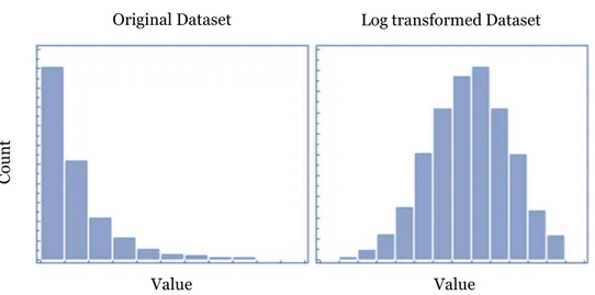
Logarithmic Transformation

Logarithmic transformation is one of the most commonly used mathematical transformation in feature engineering. It has different benefits:

• It helps to handle skewed data, after the transformation the distribution becomes more approximate to normal.

• In most of the cases the magnitude order of the data changes within the range of the data.

• It also decreases the effect of the outliers, due to the normalization of magnitude differences and the model become more robust.

Figure 11 - Example of log transformation

One-hot encoding

It is one of the most common encoding methods in ML. This method spreads the values in a column to multiple flag columns and assign 0 or 1 to them. These binary values express the relationship between grouped and encoded column. This method changes your categorical data, which is challenging to understand for algorithms, to a numerical format and enables you to group your categorical data without losing any information.

Value Value C o u n t

“Why One-Hot? If you have N distinct values in the column, it is enough to map them to N-1 binary columns, because the missing value can be deducted from other columns. If all the columns in our hand are equal to 0, the missing value must be equal to 1. This is the

reason why it is called as one-hot encoding” [8] Table 3 - Example of one-hot encoding

UserID City UserID Instanbul Madrid

UID76 Roma UID76 0 0

UID32 Madrid UID32 0 1

UID45 Madrid UID45 0 1

UID09 Instanbul UID09 1 0

UID33 Instanbul UID33 1 0

UID12 Instanbul UID12 1 0

UID75 Roma UID75 0 0

Grouping operations

In most ML algorithms, every instance is represented by a row in the training dataset, where every column shows a different feature of the instance. This kind of data are called “tidy”. There are 3 main ways to aggregate categorical columns:

• First option to select the label with the highest frequency.

• Second option is to make a pivot table. Instead of binary notation, it can be defined as aggregated functions for the values between grouped and encoded columns.

• The third and last option is to apply a group by function after applying one-hot encoding. This method preserves all the data, and in addition, you transform the encoded column from categorical to numerical in the meantime.

Numerical columns are grouped using sum and mean functions in most of the cases. Both can be preferable according with the meaning of the feature.

Feature split

Splitting feature is a good way to make them useful in terms of ML because usually datasets contain string columns that violates tidy data principles. By extracting the utilizable part of a column into new feature:

• ML algorithms able to understand them.

• Make possible to bin and group them.

• Improve model performance by uncovering potential information.

Scaling

Many times, the numerical features of the dataset do not have a certain range and they differ from each other. How can ML comprehend for example the range of two columns different as ‘Age’ and ‘Income’, how these two columns can be compared? Scaling solve this problem, the continuous features become identical in terms of the range, after a scaling process. Algorithms based on distance calculations such as k-NN or K-Means need to have scaled continuous feature as model input. Two main ways:

• Normalization, it scales all values in a fixed range between 0 and 1. It does not change the distribution of the features and due to the decreased std dev, the effects of the outliers increases. It is recommended before applying scaling to handle the outliers with care

= −₋

• Standardization scales the values and at the same time takes in consideration standard deviation. If the standard deviation of features is different, their range also would differ from each other. This reduce the effect of the outliers in the features.

= − Extracting date

Through date columns usually provide valuable info about the model target, they are neglected as an input or used nonsensically for the ML algorithms. Building an ordinal relationship between the values is very challenging for a ML algorithm if you leave the date columns without manipulation. Three possible types of preprocessing for dates:

1. Extracting the parts of the date into different columns: Year, month, day, etc. 2. Extracting the time periods between the current date and columns in terms of

years, months, days, etc.

3. Extracting some specific features from the date: Name of the weekday, weekend or not, holiday or not, etc.

1.4.3 Feature selection

It is the process of selecting a subset of relevant features to use in model construction. Feature selection is different from dimensionality reduction. Both methods seek to reduce the number of attributes in the dataset, but a dimensionality reduction method do so by creating new combinations of attributes, whereas feature selection methods include and exclude attributes present in the data without changing them.

When we deal with feature selection the objective is to choose and apply the selected features to our model to see if it works good or not. It is a fundamental part because after

having cleaned and engineered our raw data if we don’t choose the essential features to build our model all the effort made will be lost, since the model will not work as expected. Feature selection is one of the core concepts in ML which hugely impacts the performance of your model. The data features that you use to train your models have a huge influence on the performance you achieve. If on one side some features can benefit your model, on the other side some of them can affect negatively its performances.

Feature selection techniques are used for four main reasons:

• To short training times.

• To avoid the curse of dimensionality.

• To enhance generalization by reducing overfitting.

• Simplification of models to make them easier to interpret by researchers.

Now we are going to discuss the various techniques and methodologies that you can use to subset your feature space and help your models perform better and efficiently [9].

Filter methods

Features are selected based on their scores in various statistical tests for their correlation with the outcome variable. The correlation is a subjective term here.

Wrapper methods

With this method we try to use a subset of features and train a model using them. Based on the inferences that we draw from the previous model, we decide to add or remove features from your subset. The problem is reduced to a search problem. These methods are usually computationally very expensive. Some common examples of wrapper methods are forward feature selection, backward feature elimination and recursive feature elimination.

Embedded methods

These methods combine the qualities of filter and wrapper methods. It’s implemented by algorithms that have their own built-in feature selection methods. Some of the most popular methods are LASSO and RIDGE regression which have inbuilt penalization functions to reduce overfitting.

Modeling is the next phase of the traditional pipeline of a ML project. After having changed all the raw data in clean data, after having transformed and created relevant

Feature Selection

Techniques

Filter methods

Wrapper

methods

Embedded

method

features and chose the best ones, now is time to introduce the phases of model selection and hyper-parameters optimization. In the following two section we will discuss about these steps and what are the main activities to perform in order to create a good model.

1.4.4 Model selection

“In model selection tasks, we try to find the right balance between approximation and estimation errors. More generally, if our learning algorithm fails to find a predictor with a small risk, it is

important to understand whether we suffer from overfitting or underfitting.” [10]

When dealing with model selection, the attention goes to avoid two main problems: Overfitting: in the field of ML happens when

an algorithm is fitted with a certain set of examples called training test. Typically happens when we have a set of data on which we know the results and another set on which we want to predict the future results. The algorithm will achieve a level of learning that enable it to predict the set not analyzed yet. But when the fitting phase is too long or the training set is too small, the model shall adapt to characteristics unique of the training set, but that are useless for the test sets. So, the model will be very accurate for the training set but will give low performances on the test set. From the example is clear that the blue line shows overfitting characteristics with an irregular model to determine value, instead with the green line we have a stable model even with data never seen before. Underfitting: it occurs when a statistical model cannot adequately capture the underlying structure of the data. A model is underfitted when some parameters or terms that would appear in a correctly specified model are missing. For instance, underfitting would occur when fitting linear model to a non-linear data. Such a model will tend to have poor predictive performance. The red line in figure shows a model than is underfitted, we can see that it does not fit the red points as well as the green line which represents a good model that is not characterized neither by underfitting nor overfitting.

Figure 13 – Overfitting, blue line

When we build a model, we must check if the model is getting overfitting or underfitting, how we can do this? To address this, we can split the original dataset into separate training and test subsets.

This method can approximate of how well our model will perform on new data. If our model does much better on the training set than on the test set, then we are likely overfitting.

Avoid these two problems is very important to build a correct model that have optimal performances on data never seen. It is a part where the expertise of the data scientist is very crucial because to prevent these two problems, he/she can adopt different strategies, the most commons are:

Figure 16 - Model selection techniques

Model

Selection

Techniques

Cross-Validation

It is a powerful preventative measure against overfitting. The idea is to use your initial training data to generate multiple mini train-test splits and use these splits to train your model.

In standard k-fold cross-validation, we partition the data into k subsets, called folds. Then, we iteratively train the algorithm on k-1 folds while using the remaining fold as the test set called holdout fold.

Train with more data

It doesn’t work every time, but training with more data can help algorithms detect the essential features. Obvious that if we add more noisy data, this technique is useless. So before to add more data we should be always ensure that data are clean and relevant.

Remove features

Some algorithms have built-in feature selection, for those that don’t, we can manually improve their generalizability by removing irrelevant input features. It is a manual task that request time and deep knowledge of the data you are considering. It can even apply this technique with a try and error approach, testing which are the features more important with different subsets.

Early stopping

When we are training a learning algorithm iteratively, you can measure how well each iteration of the model performs. Up until a certain number of iterations, new iterations improve the model. After that point the model’s ability to generalize can weaken as it begins to overfit the training data.

Early stopping refers stopping the training process before the learner passes that point. It is a technique to avoid the overfitting.

Regularization

It refers to a broad range of techniques for artificially forcing your model to be simpler. The method depends on the type of learner (algorithm) you are using. For example, you could prune a decision tree, use dropout on a neural network, or add a penalty parameter to the cost function in regression.

Figure 17 - Cross validation technique

Ensembling

Ensembles are ML methods for combining predictions from multiple separate models. There are two main methods for ensembling:

Bagging:

• It attempts to reduce the chance overfitting complex models.

• It trains large number of ‘strong’ learners in parallel.

• A strong learner is a model that is relatively unconstrained.

• Bagging then combines all the strong learners together in order to ‘smooth out’ their predictions.

Boosting:

• It attempts to improve the predictive flexibility of simple models.

• It trains large number of ‘weak’ learners in sequence.

• A weak learner is a constrained model.

• Each one in the sequence focuses on learning from the mistakes of the one before it.

• Boosting then combines all the weak learners into a single strong learner. They are both ensemble methods but their approach to the problem is from opposite directions.

The next and last phase of the pipeline we consider is the hyper-parameters optimization. It is a very hard task aimed to improve the performances of the model selected.

1.4.5 Hyper-parameters optimization

The purpose of this step is to improve the learning process of the algorithm used to train the model. In the world of ML there are two types of parameters:

1. Model parameters

They are learned by the algorithm while learning phase. 2. Hyper-parameters

A hyper-parameter is a parameter whose value is used to control the learning process. They need to be set before beginning the learning phase.

Optimizing the hyper-parameters is a function with the objective of minimizing the loss/cost of the algorithm, which in turn keep balance between the mode bias and variance. This is essential in getting a low cross-validation error at the end of the experiment. There are different techniques to tune hyper-parameters:

Figure 19 - Hyper-parameters optimization techniques

The objective of this part is not to explain all the possible techniques in detail but to give an overview of the main techniques to adopt. The more important techniques are:

Grid Search

Grid search expects few sets of values as parameter space and tries all combinations of these values to learn in brute force manner. Search will be guided by a metric, which is often cross validation error of the training data or evaluation on the test data.

Grid Search suffers from curse of dimensionality, because even when there are two hyper-parameters and five distinct values of these hyper-parameters, it requires twenty-five times of modeling and evaluation. Besides, there is no feedback or adjustment mechanism, thus the algorithm is highly unintelligent.

Random Search

Random search is very similar to grid search and does pretty much the same, but in a random combination of hyper-parameters. It is proved to outperform Grid Search, but it performs poorly in real cases as there is not adjustment or feedback in the learning process based on the results of previous learning.

Hyper-parameters Optimization Techniques Model Free Grid Search Random Search Model-Based Bayesian Optimization Evolutionary Algorithms

Figure 20 – Grid and Random search

Bayesian Optimization

Bayesian optimization is a global optimization technique for noisy black-box functions. Applied to hyperparameter optimization, Bayesian optimization shapes a probabilistic model of the function mapping from hyperparameter values to the objective evaluated on a validation set. By iteratively evaluating a promising hyperparameter configuration based on the current model, and then updating it, Bayesian optimization, aims to gather observations revealing as much information as possible about this function and the location of the optimum. It tries to balance exploration (hyperparameters for which the outcome is most uncertain) and exploitation (hyperparameters expected close to the optimum) [11].

Evolutionary Algorithms

Evolutionary optimization is a technique for the global optimization of noisy black-box functions. In hyperparameter optimization, evolutionary optimization uses evolutionary algorithms to search the space of hyperparameters for a given algorithm. Evolutionary hyperparameter optimization follows a process inspired by the biological concept of evolution [11]:

1. Create an initial population of random solutions.

2. Evaluate the hyperparameters tuples and acquire their fitness function. 3. Rank the hyperparameter tuples by their relative fitness.

4. Replace the worst-performing hyperparameter tuples with new hyperparameter tuples generated through crossover and mutation.

5. Repeat steps 2-4 until satisfactory algorithm performance is reached or algorithm performance is no longer improving.

What we have explained until now are the general approaches to do when developing a ML model. The only things that remain to define are the metrics used to assess the goodness of a model. The next section will introduce the main evaluation methods for ML models.

1.4.6 Model evaluation

Once the model is created, the phase of testing includes the evaluation of the model based on certain metrics. Metrics are measures to define the goodness of the model according to the problem it is solving. Basically, when talking about evaluation metrics is savvy to separate the metrics used to evaluate classification models from regression models because the scopes are different and consequently even the metrics have different meanings. To have a comprehensive view of these metrics we are going to list the most important ones both for classification models and for regression models.

Classification metrics

• Confusion matrix

It is one of the easiest and most intuitive metrics to assess the correctness of a classification model. To understand this metric must be known some concept:

o TP (True Positive), TP are the cases when the actual class of the data point was True and the predicted is also True.

o FP (False Positive), FP are the cases when the actual class of the data point was False and the predicted is True.

o TN (True Negative), TN are the cases when the actual class of the data point was False and the predicted is False.

o FN (False Negative), FN are the cases when the actual class of the data point was False and the predicted is True.

Actual Value positive negative Predicted Value positive TP FP negative FN TN

Table 4 - Confusion Matrix

The objective is to reduce the more possible the FP and FN, while increasing the number of TP and TN. Once you defined these classes with the predictions of the model you implemented, then you can measure other important metrics that better describe the results of the model.

• Accuracy

The accuracy of a model refers to the number of good predictions over all the predictions made. It can be calculated thanks to the confusion matrix:

= ₊ +_{+ +}

• Precision

Precision is a measure that tells us what proportion of data points that we diagnosed as positives, and actually were positive.

= ₊

• Recall

Recall is a measure that tells us what proportion of data points that actually are positive were diagnosed by the algorithm as positive.

= ₊

• F1 Score

It is the weighted average between Precision and Recall. It is not intuitive as precision or recall metrics but F1 is more useful than Accuracy, mainly if you are considering an uneven number of classes to predict.