Assessing the operational value of forecast information under climate change

(1)

SCHOOL OF CIVIL, ENVIRONMENTAL ANDLAND MANAGEMENT

ENGINEERING

MASTER OFSCIENCE INENVIRONMENTAL ANDLANDPLANNING

ENGINEERING

A

SSESSING THE OPERATIONAL

VALUE OF FORECAST INFORMATION

UNDER CLIMATE CHANGE

Master Thesis by:

Henrique Moreno Dumont Goulart

Advisor:

Prof. Andrea Castelletti

Co-Advisor:

Prof. Matteo Giuliani Prof. Jonathan Herman Prof. Scott Steinschneider

(2)

(3)

Acknowledgments

I would first like to thank my advisor Professor Andrea Castelletti, because he is the one that made all the work and development achieved in these last eleven months possible, in addition to the support and wise suggestions that improved the overall quality of the thesis.

I would also like to thank my co-advisors. Professor Matteo Giuliani has been fundamental to this work from the very first day in so many ways that it is difficult to demonstrate how grateful I am. His guidance, assistance and kindness shall not be forgotten. Professor Scott Steinschneider, who was kind to share his knowledge on synthetic forecasts and had lots of patience to teach me how to use his model. Finally, professor Jonathan Herman, who not only allowed me to stay with his research group in Davis for a couple of (intense) months, but also provided a great deal of instruction and information, besides being always available to the many times I found myself struggling. My most sincere thanks to all of you.

Special thanks to all the researchers and colleagues at the Natural Resources Management group at Politecnico di Milano and at the Herman Research group at UC Davis, it was a pleasure to cooperate with you.

The road here has not been easy, but with friends as good as mine every-thing is manageable. I am grateful to all of them, but especially to those who were somehow involved in this work, Ivan, Kaushal, Aaron, Gabriel, Nicolas, Alexandre, Kevin and Vinicius.

Finally, I would like to reserve a special place for my family, the foundation of it all. My parents and sister, for all the unconditional love, my grandmothers, whose care and zeal have been felt even from the other side of the ocean, my grandpa, who has had an active role in revising and improving my writing and Beatriz, who has stayed by my side even after the hardest obstacles. This has been a tough yet satisfying journey. Thank you all.

(4)

(5)

Abstract

As consequence of global warming, extreme events are expected to increase in magnitude and frequency at global and local scales. In the water resources field, on top of increasingly uncertain hydrological regimes, more recurrent and intense cases of flood and drought are projected, which causes reservoirs to lose efficiency and even to fail at their purpose of supplying water and preventing floods. Forecast has been proven to be a useful tool in improving water man-agement, but little is known about its capability in future time periods under climate change. Therefore, it is the aim of this thesis to investigate the fore-cast value in the future and its contributions in mitigating the projected climate change impacts. For that, a study case at the Folsom reservoir is used, where 97 future climate scenarios are analyzed and selected according to their forecast potentiality. The selected scenarios are then simulated to establish the absolute and relative Expected Value of Perfect Information (EVPI). Given the nonexis-tence of data for future forecasts, a novel statistical framework is used to gen-erate synthetic forecasts for future time periods whilst preserving the accuracy of the existing model currently used. When combined the selected future pro-jections with the synthetic forecast framework, the future forecast ensembles for different climate change scenarios are created. In order to simulate these scenarios, a policy search framework is adopted, which applies an innovative method by controlling operation decisions with binary trees, defined by states and actions. Results indicate the use of forecast can improve water supply and prevent future floods from happening, in spite of an overall deterioration of the water operations in the future. The absolute value of forecast is projected to increase for all selected scenarios, while the relative forecast value has its evolution conditioned by the type of future scenario. In general, the relative value is expected to increase in wet scenarios but to decrease in dry scenarios. The thesis also found that forecast-based policies optimized over the past can improve the water supply levels over future time periods at the cost of increas-ing the flood risk. Moreover, given the concern about future uncertainty due to climate change, results show that forecasts allow for a wider range of future

(6)

(7)

Riassunto

Come conseguenza del riscaldamento globale, si prevede che gli eventi estremi aumentino in ampiezza e frequenza su scala globale e locale. Nel campo delle risorse idriche, oltre a regimi idrologici sempre più incerti, vengono proiettati casi più ricorrenti e intensi di alluvione e siccità, che fanno perdere alle infras-trutture le infrasinfras-trutture responsabili di attività vitali, come fornitura d’acqua e la prevenzione delle inondazioni, fallire al loro scopo. Le previsioni hanno dimostrato di essere uno strumento utile per migliorare la gestione e il fun-zionamento delle risorse idriche, ma si sa poco sulla sua capacità in periodi di tempo futuri sotto il cambiamento climatico. Pertanto, lo scopo di questa tesi è studiare i contributi previsionali per mitigare gli impatti previsti sul cambia-mento climatico nella gestione delle risorse idriche e valutarne il valore rispetto alle condizioni attuali. Per questo, vengono analizzate 97 proiezioni di afflusso per il serbatoio Folsom, basato su più modelli di circolazione generale (GCM) e percorso di concentrazione rappresentativo (RCP), quindi selezionate in base alla loro potenzialità di previsione. Gli scenari selezionati vengono simulati con una programmazione dinamica per stabilire politiche operative di base e per-fette e vengono calcolati i valori potenziali assoluti e relativi. Data la inesistenza di dati per le previsioni future, viene utilizzato un quadro statistico per gener-are previsioni sintetiche per periodi di tempo futuri, preservando l’accuratezza del modello esistente a breve termine attualmente utilizzato nel serbatoio. Se combinate le proiezioni future selezionate con il quadro di previsione sintetico, vengono creati gli insiemi di previsioni future per diversi scenari di cambia-mento climatico. Al fine di ottimizzare e simulare questi scenari, viene adot-tato un framework di ricerca delle politiche, che applica un metodo innovativo controllando le decisioni operative definiti da stati e azioni. I risultati indicano un generale deterioramento delle operazioni idriche, ma l’uso delle previsioni può migliorare l’approvvigionamento idrico e impedire che si verifichino inon-dazioni future per una serie di scenari futuri diversi rispetto a un’operazione di base. Si prevede che il valore assoluto della previsione aumenti con il tempo per tutti gli scenari selezionati in conseguenza dei maggiori costi delle

(8)

oper-negli scenari bagnati ma diminuire oper-negli scenari asciutti. La tesi ha anche scop-erto che una vecchia politica operativa supportata dalle previsioni può miglio-rare le prestazioni fino a un livello simile di una futura politica ottimizzata senza previsioni, aumentandone la durata. Inoltre, data la preoccupazione per l’incertezza futura dovuta ai cambiamenti climatici, i risultati mostrano che le previsioni consentono di contemplare una gamma più ampia di scenari futuri da un’unica politica, garantendo una maggiore flessibilità all’operazione.

(9)

4.2.1 Type of residual and preliminary tests . . . 39 4.2.2 Synthetic generation . . . 40 4.3 Forecast Value . . . 42 4.3.1 Policy tree . . . 42 4.3.2 Genetic Programming . . . 42 5 Results 45 5.1 Scenario Selection . . . 45 5.1.1 Preliminary analysis . . . 45 5.1.2 Statistical analysis . . . 49

5.1.3 Computation of the expected value of perfect information 52 5.2 Synthetic forecast generation . . . 57

5.2.1 Residual testing and selection . . . 59

5.2.2 Synthetic model . . . 64

5.3 Forecast value . . . 67

5.3.1 Historical and future forecast values . . . 68

5.3.2 Dynamics of the forecast . . . 76

5.3.3 Robustness and adaptation . . . 84

6 Conclusions and future research 89

Bibliography 93

(11)

List of Figures

2.1 Description of the steps of the Information Selection and

Assess-ment (ISA) framework. Figure by Giuliani et al. (2015). . . 9 2.2 Contribution of additional information to the overall performance

of the operation. Figure by (Giuliani, Pianosi and Castelletti, 2015). 10 2.3 Representation of both El Niño and La Niña, figure by National

Oceanic and Atmospheric Administration. . . 14 2.4 Example of an ensemble prediction system, where different

fore-casts are taken together and a better understanding of the future scenario can be obtained. Figure by Cloke and Pappenberger (2009). 16 2.5 Difference between accuracy and quality of a forecast and the

actual improvement. Figure by Li et al. (2017). . . 20 3.1 Location of the State of California and its main cities. Adapted

from Bing Maps (2019). . . 22 3.2 Distribution of runoff. Figure by Hanak et al. (2011). . . 23 3.3 California water supply system represented in the CALVIN model

scheme. Adapted from Hanak et al. (2011). . . 25 3.4 Location of the American River Basin and Folsom Reservoir. Adapted

from Herman and Giuliani (2018). . . 26 3.5 Historical rule curve of the Folsom reservoir. During winter the

conservation pool needs to be reduced to 400 TAF for flood pre-vention. . . 27 3.6 Historical register of release of water per day. Adapted from

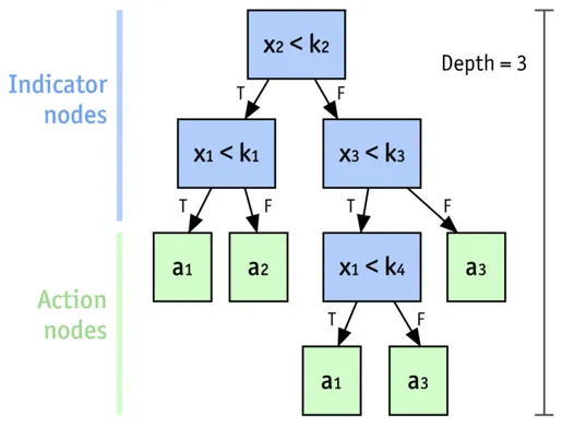
Her-man and Giuliani (2018). . . 28 4.1 General structure of the methodology used in this work. . . 36 4.2 Representation of a policy tree model. Figure by Herman and

Giu-liani (2018). . . 43 4.3 Examples of processes in the genetic algorithm. a) Crossover, b)

(12)

5.1 Daily inflow for all 97 scenarios and the mean inflow among all scenarios for a calendar year. . . 46 5.2 Boxplot with the pattern of inflows along the years 2020 until 2099. 48 5.3 Daily inflow variability with respect to the both days and years.

The anticipation of the dry period can be seen along the years as well as an increase of the flood events during winter. . . 49 5.4 Different criteria displayed in bar graphs and the selected

sce-narios in red. . . 51 5.5 Absolute and relative EVPI: Red colour stand for the relative

gains and blue colour stands for the absolute gains; Dashed lines correspond to the historical values. . . 53 5.6 Flood and drought occurrences for the historical scenario and for

the future projections. The red dots represent the selected scenar-ios. . . 55 5.7 Smoothed inflows for the entire future period, presenting trends

for each scenario. The buffer around the inflow series is the con-fidence level of 95% for each scenario at a given time. . . 57 5.8 Scatterplot between observed and forecasted inflow. Blue line is

the pattern of the data distribution and the red line indicates the perfect fit between the data. . . 58 5.9 Distribution of the forecasted inflow in relation to the observed

inflow. . . 59 5.10 Histogram for different types of residuals. Log additive residuals

present a more uniform distribution than the others. . . 60 5.11 Normal Q-Q plots for different types of residuals. Additive

resid-uals present a more uniform distribution. . . 60 5.12 Autocorrelation function for different types of residuals.

Addi-tive residuals show longer memory. . . 61 5.13 Partial autocorrelation function for different types of residuals.

Normal additive residuals are the only showing negative PACF values and longer memory. . . 62 5.14 Heteroskedasticity function for different types of residuals. Only

additive residuals show heteroskedasticity. . . 63 5.15 Scatterplot presenting the forecasted inflow based on the observed

inflow. Black triangles represent the historical data and the red circles the synthetic generated. . . 65

(13)

List of Figures

5.16 Relationship between the residual inflow and the observed in-flow. Black triangles represent the historical data and the red circles the synthetic generated. . . 65 5.17 Histogram with magnitude and frequencies of the residuals for

both historical and synthetic cases. Black represents the historical data and red the synthetic generated. . . 66 5.18 Autocorrelation functions for observed residuals and synthetic

residuals for both summer and winter seasons. . . 67 5.19 Operating costs for different scenarios and time periods. The

black bar represents the baseline operation without forecast, the blue bar stands for the perfectly-informed operation and the red dot shows the actual operation with the use of forecast. The black X represents scenarios that have flood events and penal-ties linked to it. . . 69 5.20 Costs reductions and fractions in a normalized space for the

dif-ferent scenarios. The black bar represents the baseline operation cost without forecast as 1.0, the blue bar indicates the maximum reduction possible with a perfectly-informed operation and the red dot shows the actual reduction of the operation cost when using forecast. . . 70 5.21 Forecast gain for both historical and future time periods in

ab-solute terms,(TAF/day)2. Black square stands for the historical forecast improvement with respect to a baseline operation, red triangle stands for the operation in a future time period. Note that for the sake of readability, the gain of future wet scenario which allows avoiding the flood event is rescaled and marked with a black cross. . . 71 5.22 Forecast gain for both historical and future time periods in

rel-ative terms, based on the baseline operation without forecast. Black square stands for the historical forecast improvement with respect to a baseline operation and red triangle stands for the op-eration in a future time period. . . 72 5.23 Temporal evolution of the forecast gain between a historical time

period and a future time period. The red triangle stands for the gain of forecast in the future, while the black square represents its gain in a historical time period. If the red triangle is closer to one than the black square, it means the value increased in time, otherwise, it lost value. . . 73

(14)

5.24 Assessment of the forecast gain for different scenarios along time. The red triangle stands for the gain of forecast in the future, while the black square represents its gain in a historical time period. If the red triangle is closer to one than the black square, it means the value increased in time, otherwise, it lost value. . . 74 5.25 (a) Analysis of the forecast gains when compared to extreme events

such as floods and droughts. Blue triangles stand for the number of days in a year of floods and red circles represent the days in a year with a drought. The two lines stand for the linear regres-sion of the two data sets, blue for the flood cases and red for the drought cases. (b) illustrates the forecast gain in time, varying in color, with the temporal deviation of the two types of events, flood and droughts, between the past and future time periods. . 75 5.26 Storage levels for a dry scenario in the future. (a) Comparison

between the storage levels managed by the baseline operation, the black line, and the forecast operation, blue line. Rule curve stands for a static ruling policy; (b) Release scheme during a wet season, being the dashed line the water demand; (c) Compari-son between the storage levels of the actual forecast (blue line) and the perfect forecast operation (green line). The background colors represent the type of action taken by the policy: red for hedging, blue for releasing excess and light yellow for releasing the demand. . . 77 5.27 (a) Storage levels in a wet scenario managed by the baseline

oper-ation, black line, and the forecast-based operoper-ation, blue line. (b) and (c) show the moment when a flood happens. (d) Compari-son between the synthetic forecast operation (blue line) and the perfect forecast operation (green line). The background colors represent the type of action taken by the policy: blue for releas-ing excess and light yellow for releasreleas-ing the demand. . . 79

(15)

List of Figures

5.28 (a) Storage levels during a dry season in a dry scenario for both baseline (black line) and forecast-based (blue) operations, with the latter storing more water than the former. (b) Corresponding period of time for release of water by the dam in both operations and the demand curve of water for the same period (dashed line). (c) Comparison between the storage management for both oper-ations using an actual forecast (blue line) and a perfect forecast (green line). The background colors represent the type of action taken by the policy: red for hedging, blue for releasing excess and light yellow for releasing the demand. . . 81 5.29 (a) Storage levels in a dry season of a wet scenario for both

base-line (black base-line) and forecast-based (blue) operations, with the latter storing more water than the former. (b) Corresponding pe-riod of time for release of water by the dam in both operations and the demand curve of water for the same period (dashed line). (c) Comparison between the storage management for both oper-ations using an actual forecast (blue line) and a perfect forecast (green line). The background colors represent the type of action taken by the policy: red for hedging, blue for releasing excess and light yellow for releasing the demand. . . 83 5.30 Comparison between the resulting policy for the wet scenario in

the historical time period (a) and the policy for the same wet nario but now in the future period (b); Example of how two sce-narios can generate different actions for a similar state, (c) is the policy for a wet scenario, while (d) is the one for a dry scenario. 85 1 Estimation of costs by the perfect forecast, the ensemble and

sin-gle trace. The grey line stands for the standardized perfect-operation cost, while the markers represent how much more expensive the operations are for each case. The traced blue line illustrates the difference in cost between the ensemble and a single trace policy. 99

(16)

(17)

List of Tables

3.1 Table illustrating the costs of each scenario for different types of

policy. The columns show the type of model used and the rows define the type of scenario for each time period. . . 30 3.2 State variables used for the policy tree algorithm. . . 31 3.3 Actions that can be taken for each policy. The rule curve is

lim-ited to either releasing demand or hedging a variation of p and three-day forecast policy has an additional action to anticipate floods. . . 32 3.4 Changes required in the parameters to allow for the proper

sim-ulations of each case. . . 32 3.5 Common parameters for the entire simulation. . . 33 5.1 Statistical characteristics to be assessed, the scenarios selected

and the frequency of these scenarios as the most suitable for each index. . . 50 5.2 All scenarios selected, their model names and RCPs. . . 50 5.3 Correlation between indices used at this work and the ones from

RClimDex. . . 52 5.4 Perfect operation policy and basic operation policy performance;

the absolute EVPI and relative EVPI computed over the selected future scenarios and over the historical period. . . 52 5.5 Correlation between the two types of performance gain and the

various indices indicating different properties of the scenarios. Positive correlation for the absolute gain are variance and flood length. For the relative gains flood indices and mean are pos-itively correlated and drought negatively correlated. Relative gains seem to be more influenced by the climate conditions than the absolute gain. . . 54

(18)

5.6 Table illustrating the properties of each selected scenario. The columns show the scenarios representing the three types of groups: dry, wet and intermediate and the two extra scenarios driest and wettest. The rows are for the main characteristics of each scenario. 56 5.7 Comparison of the total operating costs between the forecast

pol-icy optimized in the past and the past baseline for simulations during the future time period. . . 86 5.8 Analysis of robustness from a flood prevention perspective. The

columns describe the optimize policy and the rows describe the simulated scenario. The Verdict scenario indicates if the given scenario suffered from flood events under any policy and the Verdict policy indicates if the corresponding policy results in flood events for any type of scenario. . . 86 5.9 Analysis of robustness from a water supply perspective. The

columns describe the robust policy obtained in table 5.8 and the the baseline policies, in historical and future periods, while the rows describe the simulated scenarios. . . 87 1 Table illustrating the costs of each scenario for different types of

policy. The columns show the type of model used and the rows define the type of scenario for each time period. . . 98 2 Table highlighting the difference in values between the ensemble

of forecasts, a single trace and the perfect policy. The rows define the type of scenario for each time period. . . 98

(19)

(20)

(21)

1

Introduction

1.1 The context

The planet earth has been experiencing a constant increase in its temperature along the past decades, both on land and on the ocean surface. It is estimated that an average warming of 0.85◦C has taken place since 1880 to present-day (IPCC, 2018). The increase in temperature has had reflections on acidification of the oceans, loss of ice sheets on both poles, rise of mean sea level, among other consequences (IPCC, 2014).

There are no records of any similar event to the present one and there is a plethora of evidences that relates global warming to an abrupt increase of greenhouse gas (GHG) concentration levels, which in turn have their roots at human-related activities, especially from 1750 onwards, with half of the cu-mulative anthropogenic CO2 emissions taking place in the last 40 years (IPCC, 2014). Emissions come mainly from electricity and heat production, industry, transport and agriculture, forestry and other land use. In addition, two factors stand out as the main drivers of CO2 emissions: human growth and economic growth, the latter presenting an ever-increasing contribution (IPCC, 2014).

Changes observed in temperature and climate carry consequences into the environment. Different species have altered their natural behaviour as a reac-tion to climate change, while hydrological systems are being affected due to snow melting, oceans are suffering from acidification, and certain crops have

(22)

had their yields negatively disturbed (IPCC, 2014). Moreover, it is expected that water scarcity and stress cases will grow in many regions around the world. The tendency is to observe increased occurrences of floods in certain regions, as a result of more frequent extreme precipitation events and to observe harsher droughts for longer periods (multi-decade) in other regions (IPCC, 2014; Dama-nia et al., 2017).

On top of that, the global population is expected to keep growing during this century. In spite of the variability of growth projections, it is predicted that a net value of one billion people will be added to the world by 2030, which makes for a total of 8.6 billion people. Furthermore, by the end of the century the total population should be around 11.2 billion people, increasing by 3.6 billion with respect to the current population (United Nations, 2017). While de-veloped countries are growing at slower rates, especially in Europe, the main population growth will take place in countries in Africa and South Asia. At the same time, a different process is taking place, the rural flight. Migrations from rural areas to urban areas all over the world will add 2.4 billion people to cities by 2050 (FAO, 2017). This increase in human population implies naturally a greater demand for food and the expansion of cities translates into a bigger demand for sanitation and energy, all of which will accentuate even further the stress on water resources, given their role in agriculture, sanitation and power generation (FAO, 2017). Thus, the demand of energy keeps rising, concurrently with a need for decarbonising its sources, which contributes to the expansion of clean and renewable sources. Hydropower is a key supply in the energy production, being the major source of renewable energy, corresponding to 58% of the total global renewable energy generation (IRENA, 2018).

In this context, the importance of water-control structures, such as water reservoirs is growing (Zarfl et al., 2014; Culley et al., 2016; Ehsani et al., 2017). However, simply expanding the infrastructure capacity of dams might prove costly and not-necessarily effective, since the infrastructure investment is ir-reversible and might not meet the future water supply needs. This is due to the amplified uncertainty of future projections, which prevents an accurate comprehension of the climate conditions in the long-term future (Fletcher et al., 2019). Thus, as an alternative to the construction of water reservoirs, it is pos-sible to act on the operation of the reservoirs, representing a low-cost and flexi-ble solution that can improve the resilience of the system against the increased variability of future conditions (Castelletti et al., 2008; Ramos et al., 2013; Giuliani et al., 2016).

(23)

1.2. Objectives of the thesis

Reservoir operations are traditionally managed based on historical records, such as precipitation, temperature, day of the year and daily demand. How-ever, because of climate change, the patterns for hydrometeorological states change in multiple and unprecedented forms. Hence, the traditional approach loses reliability and performance, since it cannot effectively control the releases of water in a scenario where the hydrological conditions behave differently from what was historically defined and is more prone to system failures (Geor-gakakos et al., 2012; Turner et al., 2017). Because of that, an adaptive management strategy is needed. This approach consists in constantly receiving new data, ei-ther observations from a physical state or future predictions based on models, related to the hydrological conditions at the moment of the operation and using it for informing operational decisions. Studies (Georgakakos et al., 2012; Culley et al., 2016; Giuliani et al., 2016) showed that different concepts of the adap-tive method did improve the operation with respect to the traditional method. Among them, forecast systems excels as one of the most studied tools in wa-ter operations. The forecast value has been verified in different occasions and circumstances, be it for flood prevention using short-term models (Adamowski, 2008; Cloke and Pappenberger, 2009), water supply supported by long-term fore-cast information (Hamlet and Lettenmaier, 1999; Mahanama et al., 2011; Yuan et al., 2015) or for different types of reservoirs (Turner et al., 2017; Anghileri et al., 2016). Its flexibility allows for large ensembles of physical forecasts to be coupled for more accuracy (Pappenberger et al., 2008) or to rely on statistics to generate the predictions (Toth et al., 2000; Block and Rajagopalan, 2007). Building on these mentioned studies, the main interest of this work concerns moving the assess-ment of forecast from the present to the future time period, in which the uncer-tainty is intensified and extreme events are more likely to occur. Particularly, to understand if a forecast system is able to keep the properties and contributions seen in the current time and, furthermore, if it is capable of mitigating the neg-ative impacts of climate change by reducing the occurrences of system failures and extending the lifespan of the structure.

1.2 Objectives of the thesis

As previously explained, even though there are plenty of studies supporting the benefits of using forecasts in water-control operations (Georgakakos et al., 2012; Denaro et al., 2017; Turner et al., 2017; Nayak et al., 2018; Herman and Giuliani, 2018), they usually focus on the use of forecast for past or current scenarios. In such cases, in spite of the benefits already being significant to the improvement

(24)

of regular operations, little can be learned or applied to the incoming future, where projections heavily differ from historical records and the states of the climate variables are harder to predict.

This study has the primary goal of exploring the forecast value in future con-ditions affected by climate change and to assess in which ways it differs from the current contributions estimated over historical conditions. Specifically, the research questions that guide this work are:

1) How water systems operations and their performance will be impacted by climate change?

2) Can forecast contribute to design adaptive operating policies?

3) Is the forecast value expected to increase under future and more variable hydroclimatic regimes?

4) How sensitive is the forecast value across an ensemble of uncertain sce-narios?

5) Can an adaptive policy over a historical conditional provide satisfactory results when evaluated in the future? Is the addition of a forecast enough to extend its usefulness?

The case study of the Folsom reservoir, near the Sacramento city in Cali-fornia (United States of America) is used to test the proposed methodology. California is a state that has historically faced water-related problems, such as extreme shortages of water that can exceed the duration of years and severe floods affecting its many cities and inhabitants. Folsom reservoir is an artificial reservoir constructed in 1955 and located on the American River. Nowadays, the reservoir serves multiple objectives, but its main tasks are still flood control and water supply operations.

In order to achieve the ultimate goal of evaluating the benefits of forecast in a future scenario affected by climate change, some intermediate and specific objectives need to be set as well, which are:

1) Analyzing the projected climate and understanding the main trends in terms of variability and predictability, frequency and duration of extreme events.

(25)

1.3. Outline of the thesis

2) Quantifying the maximum space of improvement of the historical op-erations with respect to an ideal solution designed assuming a perfect (deter-ministic) knowledge of the future, also known as Expected Value of Perfect Information (EVPI; Giuliani et al. (2015)).

3) Generation of a synthetic forecast ensemble for projected reservoir inflow based on the work of Nayak et al. (2018). The synthetic generation allows for a reliable simulation of the existing forecast models over projected inflow sce-narios.

4) Quantifying the actual forecast value as the performance gain generated by informing the Folsom reservoir operations with the synthetic forecast over the historical and future scenarios.

1.3 Outline of the thesis

Chapter 2 describes the state-of-the-art on the topic of metereological and hy-drological forecasting in water systems. It starts with the definition of value of exogeneous information for water systems operations. It then describes the types of existing forecasts, discussing skill, lead time, uncertainty, and the rela-tion between forecast skill and forecast value. A brief explanarela-tion of reforecast, hindcast and synthetic forecast is also provided.

Chapter 3 provides a comprehensive description of the Folsom reservoir case study. Firstly, the morphologic and hydro-climatic features of the Califor-nia river basin are presented. Then, a summary of the stakeholders and the main interests involved in the system is provided. Finally, the data utilized in the study are described.

Chapter 4 illustrates the proposed methodology, which is composed of the following three main blocks: 1) Scenarios selection based on a statistical anal-ysis of the climate projections coupled with the quantification of EVPI; 2) Syn-thetic generation of inflow forecast for the selected scenarios; 3) Assessment of historical and future forecast value.

Chapter 5 reports the numerical results obtained in this study. According to the proposed 3-block framework, it first discusses the scenairo selection based on the projected climate statistics and the values of EVPI; the synthetic forecast generated for the selected scenarios are then reported; finally, it analyzes the

(26)

historical and projected forecast value.

Chapter 6 sums up the conclusions and suggests some starting points for further research about the topic.

(27)

2

State-of-the-art

2.1 Value of observation

Today there are many technologies, tools and methods that improve the man-agement and operation of water resource systems. In a world with a surfeit of data available, one of the most common practices is to harness real-time data and observations, which can be achieved by using a variety of equipment, such as radars, sensors, satellites or even touristic webcams (Giuliani et al., 2016), in order to gather additional useful information that allows for an enhanced operation. For water resources operations, relevant observable information can be for instance precipitation, upstream flows or snow pack depth (Denaro et al., 2017). Similarly, Giuliani et al. (2016) developed a low-cost, real-time and observation-based method for extracting snow-related information from pic-tures on the web taken from users and webcams. After an automatic process where the pictures are localized, processed and analysed, a virtual snow index is computed to represent the snow-covered area. This index is embedded into the system operations and it produced an improvement of 10% in relation to the baseline operations (Giuliani et al., 2016).

Even though direct observations cannot foresee future trends of inflow with great accuracy, the potential for directly using hydro-meteorological data is be-coming relevant as indicated by Denaro et al. (2017). Their study showed that by knowing solely the accumulated snow state on the mountains during winter, it was possible to anticipate the amount of water to be melted during spring,

(28)

ultimately permitting a larger amount of water to be stored for providing re-liable irrigation over the summer. The higher water levels of the lake led to an improvement of the water supply index of 10% in relation to the baseline scenario, in spite of an increased risk of flooding. In another study concerning flood events in the north of Italy, Castelletti et al. (2008), added to a traditionally-designed policy real-time information, e.g., precipitation and temperature mea-sures. While the results presented modest improvements with respect to the regular policy performance during the flood season, this solution largely im-proves the system performance during the rest of the year.

However, even though better informing the operations of water systems has its benefits, it also carries some drawbacks, such as observational error and estimation biases, possibly negatively affecting the system performance. To support the selection of the most useful information for improving the system operations, Giuliani et al. (2015) developed the information selection and as-sessment (ISA) framework. Figure 2.1 illustrates the process and it works as following: first the expected value of perfect information is determined as the difference between an ideal, perfect solution designed under perfect knowl-edge of the future and a baseline solution relying on a basic set of information. Then, multiple candidate information are processed by an input variable selec-tion algorithm to automatically identify the ones that are expected to be more valuable for informing operational decisions. Lastly, the selected variables are used in designing informed solutions. The operational value of this informa-tion is quantified as the the performance gain of the informed soluinforma-tions with respect to the baseline.

(29)

2.1. Value of observation

Figure 2.1: Description of the steps of the Information Selection and Assessment (ISA)

(30)

Whilst the original intended use of the ISA framework was to identify and select the most valuable information from a set of observational data, it can also be exploited for forecasts identification and selection. The process and steps would remain the same, but the candidates in the second step of the frame-work would instead be different forecast models, different forecast variables, or different forecast lead times.

Figure 2.2: Contribution of additional information to the overall performance of the operation.

Figure by (Giuliani, Pianosi and Castelletti, 2015).

2.2 Forecasting

2.2.1 Forecasting in water resources operations

Although it is possible to predict future conditions, such as flood events, only by relying on weather observations, there are situations in which a forecast model is necessary. It might happen that the equipment fails or it might be that the basin is located in an area where the conditions are hard to be measured (Toth et al., 2000). Furthermore, studies have shown that with the help of fore-cast models, water supply failures were reduced and the life-spam of hydraulic infrastructure was increased, all at a relatively low cost, when compared to new

(31)

2.2. Forecasting

investments in new infrastructure (Turner et al., 2017).

Along the past fifty years, there was a considerable improvement in weather forecasting, with great advances in lead times, forecast skill and value. This progress is directly linked to the considerable increase in computing power, in-strumentation and understanding of the atmospheric dynamics (Lynch, 2008). Plenty of researches have been published analysing the multiples contributions of forecasting to the water resources operations, including different objectives like flood control, water supply, hydropower generation and different combi-nations of them together. Some of these studies are recalled and briefly ex-plained in this section in order to provide evidences of the importance of fore-casting in this domain.

A study by Faber and Stedinger (2001) presented the implementation of fore-cast into a Sampling Stochastic Dynamic Programming (SSDP) model and how it performed in comparison to a standard operation. In fact, two alternatives were developed: A SSDP model calibrated on the historical conditions, but in-corporating current hydrologic information forecasts to update the probabili-ties and a SSDP model using ensemble streamflow prediction (ESP) updated on a weekly basis. Both presented a superior performance in relation to the base-line case, the same system and model but without the forecast components. Plus, some differences in the output of the two forecast models were found, with the one using the ESP outperforming the solution based on historical con-ditions but updated with current hydrologic information forecasts (Faber and Stedinger, 2001).

Anghileri et al. (2016) recently studied the value of long-term forecasts in the design of water supply operations, by using a forecast-based adaptive control framework. The first results showed that season-long ESP forecasts improved operations with respect to the baseline, remaining 35% below the perfect fore-cast value. The system considered in this study (i.e., the Oreville reservoir, California) allows storing water from one year to the other and would have here gained much more from forecast over longer lead-time than the seasonal one. In fact, the inter-annual component of the forecast contributed from 30 to 45% of the total forecast value. Moreover, it was possible to analyse in which circumstances each type of forecast generated most value with respect to the baseline (no forecast): for high demands with respect to the storage capacity or inter-annual carryover, only a perfect forecast would be able to properly an-ticipate the streamflow; medium-high demands but a small storage was

(32)

suffi-cient for the seasonal ESP forecast to perform and finally, inter-annual forecasts worked best for big storages, in spite of not being useful for small reservoirs (Anghileri et al., 2016).

It is also worth noticing that the gains to the water operations provided by forecasts depend also on the final objective of the water reservoir, as shown by Turner et al. (2017). For flood-prevention operations, for instance, increasing the quality of forecasts directly implies in an improvement to the system’s per-formance. However, for water supply purposes, the correlation is not as clear, because some reservoirs are capable of buffering the variability of the inflow. In addition, smaller reservoirs, which have less buffering capacity, are the ones that would profit the most of long-term forecast (Turner et al., 2017).

Another example demonstrating the value of forecast is provided by Nayak et al. (2018) for the operations of Folsom Reservoir (California), in which it was possible to considerably improve the reliability of water supply without in-creasing the risk of floods due to the prediction of major flood events by a fore-cast model. However, the study found that forefore-casts with a skill of thirty days did not present significant improvements in relation to forecasts with a three-day skill for the river basin studied. Finally, it was suggested that forecasts can also bring advantages to conjunctive use, such as groundwater storage in water reservoirs, because of the longer times required for water banking and withdrawing from underground storages (Nayak et al., 2018).

2.2.2 Forecast lead time

Forecasts are usually divided in two categories: short-term and long-term or seasonal. The first ranges from one day to five days, rarely exceeding one week, while the second ranges from months to multiple years. Each category has its own objectives, because it is still a challenge to integrate the different time-frames in a single model (Yuan et al., 2015). The dynamics in each case change substantially and so do the main factors contributing to the forecast skill. In short-term predictions, the forecast horizon, which quantifies the number of days in advance that can be foreseen, is the most important factor. Gener-ally, the longer the forecast horizon the better is the performance of the system. However, for long-term forecasts, the forecast uncertainty plays the main role, as the forecast can become too uncertain at long lead times. At medium fore-cast horizon, the performance of the system is equally affected by both factors (Zhao et al., 2012).

(33)

Short-term forecasts are mostly aimed at alerting flood occurrences and at mitigating the impacts related to them. The few days of anticipation allow for releasing water from reservoirs, so the flood can be partially diminished, con-tributing to a reduction of the damage to people, buildings, agriculture, and infrastructure (Pappenberger et al., 2008; Elsafi, 2014). Short-term forecasts can be based on direct observational data through the use of radars and gauges to capture the precipitation state or on more advanced models, such as numeri-cal weather prediction and ensemble prediction systems that ensures accuracy, quickness, reliability and robustness of the forecast system (Adamowski, 2008; Cloke and Pappenberger, 2009).

On the other hand, long-term forecasts address concerns that are not as im-mediate or urgent as the short-term, but still of great importance to the envi-ronment and society, such as water supply and power generation. For these, it is important that the forecast can predict the future states at longer time leads, such as months, seasons, and years. Long-term forecast mostly rely on slow cli-mate dynamics and, consequentially, require different weather information to be acquired. Among them, snow state information and soil moisture data have been proved to be useful at extending the forecast skill to longer lead times for specific regions. As an example, a study by Mahanama et al. (2011) found that in some regions of the United States of America, the contributions of soil moisture and snowpack initialization allowed for skillful forecasts with 95% confidence level of up to 9 months of lead time during certain seasons (Mahanama et al., 2011).

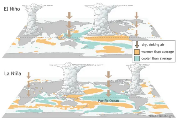
Nonetheless, such correlations are limited to specific regions and seasons. At the global scale the understanding of ocean-atmosphere teleconnections is paramount and nowadays, most long-term forecasts rely on understanding teleconnection patterns (Yuan et al., 2015). The term describes a naturally-occurring climate variation or alteration, such as the sea surface temperature (SST) fluc-tuation of the oceans, that affects different regions globally, usually at long dis-tances and for multi-year periods of time (Nigam and Baxter, 2014). Among teleconnection patterns, the El Niño Southern Oscillation (ENSO) is one of the major ones, affecting the whole planet in different ways. It involves sea sur-face temperature (SST) oscillation along the years, with a warm-phase called el Niño and a cold-phase called La Niña, as seen in Figure 2.3. The return fre-quency varies from 4 to 6 years and lasts for 2 years. Forecasts based on ENSO were shown to keep the skill from 6 to 9 months of lead time for some regions along the coastline of the Pacific Ocean (Hamlet and Lettenmaier, 1999).

(34)

Figure 2.3: Representation of both El Niño and La Niña, figure by National Oceanic and

Atmospheric Administration.

Yet, some regions are not substantially affected by the ENSO, as is the case of the European continent. During the colder months of the Northern Hemi-sphere, another phenomenon becomes predominant in the atmospheric vari-ability, which is known as North Atlantic Oscillation (NAO). It is a large-scale reorganization of the air masses located in the Arctic and subtropical Atlantic. Every movement alters the average speed, direction, temperature and moisture of the air currents in the region and even storms are regulated by the NAO. The phenomenon has two phases, a positive one and a negative one and the consequences can be observed for instance in fish population, agricultural har-vests, water management and energy supply (Hurrell et al., 2003). Furthermore, when basing forecasts on NAO, it is possible to predict winter discharges with relatively high skill in some regions of Europe and also subsequent summer discharges, but at lower skill (Bierkens and van Beek, 2009).

One of the first researches studying teleconnections at water resources oper-ations was the work by Hamlet and Lettenmaier (1999), which aimed at exploring the potentiality of long lead climate forecasts to improve river operations in the United States of America. By coupling the El Niño Southern Oscillation (ENSO) and the Pacific Decadal Oscillation (PDO), to the streamflow forecast ensemble, it was verified that a 6-month forecast was achieved for the Columbia River.

(35)

Furthermore, the study showed that this addition of forecast would bring ben-efits to hydropower generation, water supply for agriculture activities, fisheries management and flood control (Hamlet and Lettenmaier, 1999).

2.2.3 Types of forecast models

A model is a simplified copy of a real system that has as purpose to mimic it, in order to represent as realistically as possible the experiments conducted and to generate reliable results, which can then be used as base for other experi-ments, tests and researches (Soncini-Sessa, 2007). There are many types of mod-els, which are duly described in the study by Jajarmizadeh et al. (2012). In the realm of hydrological forecasting, however, there are two main approaches, the first relying on physically-based models and the second on data-driven models. Physically-based models, also known as dynamic, process-based climate models aim at reproducing specific climate patterns and dynamics, as atmo-spheric pressure, temperature, precipitation, so a future state can be foreseen. A classical example is the numerical weather prediction (NWP), one of the most traditional models for the forecasting of climate states, such as precipitation. The outcome of the NWP can then be used as input for hydrological models, which will allow ultimately to predict a river flood event. While the dynamic models usually lead to better responses of a water system, its uncertainty is still considerable, with high chances of missing flood events or providing false alarms, especially at longer lead times (Zhao et al., 2012). A way to solve the vulnerability is to conceive an ensemble of forecasts or an ensemble prediction system (EPS), in which multiple predictions of possible states are put together, providing different values of forecasting and thus giving a broader idea of the upcoming climate state, as can be seen in Figure 2.4 which will serve as infor-mation for a hydrological model. Studies showed EPSs contribute to the value of forecasting at medium-range, presenting a better performance at identifying floods events for longer lead times (Cloke and Pappenberger, 2009; Pappenberger et al., 2008). Albeit, while EPS improved results, relying on a single Ensem-ble Prediction System might still offer some vulnerabilities motivating the use of multiple EPS together, also known as grand-ensemble. Pappenberger et al. (2008) used the THORPEX Interactive Grand Global Ensemble (TIGGE), which is composed of seven ensembles, to reduce the vulnerabilities of the system and attained an improved performance with respect to a single EPS, forecasting up to 8 days in advance flood events (Pappenberger et al., 2008).

(36)

Figure 2.4: Example of an ensemble prediction system, where different forecasts are taken

together and a better understanding of the future scenario can be obtained. Figure by Cloke and Pappenberger (2009).

The concept of ensembles can be applied as well for forecasting river in-flows, which is called ensemble streamflow prediction (ESP), developed by the National weather service (NWS) since 1970 (Yuan et al., 2015). It consists in combining the physical-based model of a river at the given moment, where current conditions are taken into calculations, with the climate data from many historical years, culminating into a set of patterns or traces that could possi-bly take place, each one based on a different year (Faber and Stedinger, 2001). Later, with the increase of computing capacity and better understanding of globally occurring phenomena, such as teleconnections, the general circula-tion models (CGCMs) were conceived, describing globally the behaviour of atmosphere, ocean and land in an integrated way. Alongside the traditional ESP, this allowed for the creation of the climate-model-based seasonal hydro-logic forecasting (CM-SHF). It benefits from the ensembles of trajectories of the ESP for precipitation and temperature, but at longer lead times, because of the higher capacity of the CGCM at predicting season-long climate states (Yuan

(37)

et al., 2015).

The second class of forecast models are the data-driven models, also known as black box models. The idea behind data-driven models is to determine cor-relations between data, by applying different mathematics operations, without necessarily explaining the physical and chemical processes involved. The most common and basic type is the linear regression model, in which different data are coupled and correlated in a linear way. Among the drawbacks of linear regression, it is worth mentioning the impact of outliers and the inability to capture non-linear correlations between the data (Block and Rajagopalan, 2007). Another data-driven model commonly used is the autoregressive moving aver-age (ARMA) model, which establishes a linear relation between different time-steps of the same data, predicting future values based on past observations (Toth et al., 2000).

An alternative proposed by Block and Rajagopalan (2007) was to utilise a lo-cal polynomial-based nonparametric approach, overcoming some of the lim-itations of linear-regression models, being more flexible and able to capture other trends. The method allowed for the selection of the nearest neighbours of a specific point of interest, then locally parametrizing the data with a poly-nomial function and finally adding random deviates with the same standard deviation of the polynomial to generate an ensemble. The advantages of this method are the minimization of outliers’ disturbance, detection of local corre-lations and elimination of multicollinearity, when one variable is correlated to multiple other variables (Block and Rajagopalan, 2007).

In addition, two other data-driven models deserve to be briefly discussed. The K-Nearest-Neighbour Method (KNN) explores the closest data to a specific observation in a data sample and establishes the correlation between them. It is a non-parametric approach and does not establish any structural relation-ship between the data sets (Toth et al., 2000). The second model, Artificial Neu-ral Network (ANN), is a computer intelligence trained at recognizing relation-ships between inputs and outputs. This method does not require any a priori hypothesis and works with any sort of relationship between the data sets, in-cluding non-linear and complex ones. Many studies showed ANN overcoming the more basic methods such as ARMA and linear regression (Toth et al., 2000; Adamowski, 2008; Elsafi, 2014).

(38)

past decades, there is still no clear evidence of outperformance of one model over the other, with each one presenting different benefits and disadvantages to the other. Physical models are precise, give better understanding of the natu-ral processes involved and can simulate a variety of flow situations, but require more data to be set, which is not always possible and cannot take exogeneous data into account (Elsafi, 2014). Data-driven models are usually quicker, sim-pler and easier to operate, but are restricted to stationary data, which makes it particularly limiting for the current climate change context (Adamowski, 2008).

2.2.4 Forecast uncertainty

Meteorological and hydrological forecasting can contribute to the improve-ment of water systems in different ways, such as alerting for floods and prepar-ing for droughts, by anticipatprepar-ing the upcomprepar-ing conditions and extreme events. However, forecasts cannot provide flawless predictions and there is a need to assess and measure the uncertainty of the predictions, fully understanding the uncertainty of a forecast can actually further improve its value and reduce mis-lead decisions (Ramos et al., 2013).

Better understanding of forecast uncertainty means incorporating additional information into the expected forecast prediction. Instead of only providing what the future value is expected to be, the uncertainty allows communicat-ing the confidence interval of such value. Results by Ramos et al. (2013) suggest that decisions by operators were taken based on both forecasted values and un-certainty information show how the higher the unun-certainty of a prediction, the more conservative the decisions taken were. Moreover, the same study pointed out that with uncertainty information, more optimal decisions were taken, im-proving the overall performance of the system (Ramos et al., 2013).

A model can have many sources of uncertainty. Generally, the major source of uncertainty of a long-term forecast is the one related to the meteorological input (Cloke and Pappenberger, 2009). Observational uncertainty, which is related to the data assimilation, is also relevant because of the temporal and spatial uncertainties that can alter the system. Among the other sources of uncertainty, there are the geometry of the system and the characteristics of it, which are represented as parameters in the model and can be wrongly defined. For a more extensive discussion on the different types of uncertainty, refer to Cloke and Pappenberger (2009).

(39)

2.2.5 Forecast skill and value

There are two important factors when assessing the usefulness of forecasts: skill and value. The forecast skill is defined as the ability of the model of accu-rately predict the streamflow that will actually occur within given upper and lower bound (Hamlet and Lettenmaier, 1999). Thus, a skillful forecast implies that the value observed is within the estimation boundaries of the forecast model. The skill relies solely on the capacity of the forecast model and because of that, over the past 50 years, there has been a continuous improvement with the de-veloping of new technologies and models (Lynch, 2008).

Skill alone is not enough to determine the quality of a forecast. For example, two forecasts with similar skill can generate different results for a water oper-ation and there are cases in which, even if there is a perfect forecast with con-siderable skill, the operation might not change substantially because of other factors, such as structural limitation. An example is the case of a reservoir with a small storage capacity with respect to the incoming flood volume, which will not be able to buffer the flow peak even if this is perfectly forecasted (Anghileri et al., 2016). The relationship between the forecast and the actual improvement to the operation is called forecast value. It is computed by comparing the sys-tem performance with the forecast and without it.

In a study on farmers decisions based on forecasts, Li et al. (2017) identified a clear non linear relationship between skill and value; moreover, they showed that most of the state-of-the-art weather forecast products still presented a lim-ited accuracy for long-term forecasts. This inaccuracy generates doubts among farmers about forecast reliability and based on that, the quality of forecast did not necessarily improve proportionally the operation performance. On the other hand, farmer behaviour was shown to be a relevant variable influenc-ing the estimated forecast: while a risk-neutral profile presented an increase of 3% with respect to the baseline case, a risk-prone profile experienced 10% of increment, since the operator was taking a bigger risk and relying more on the forecast result (Li et al., 2017).

(40)

Figure 2.5: Difference between accuracy and quality of a forecast and the actual improvement.

Figure by Li et al. (2017).

In a similar study exploring forecast skill and value for water supply, Turner et al. (2017) suggest that in order to minimize the risks of a misleading forecast and to potentialize its value, it is recommended to have long records of data and a large number of reforecasts (Turner et al., 2017).

(41)

3

Study site

3.1 California

The state of California is located on the west coast of the United States of Amer-ica and bordered by Mexico to the south (Figure 3.1. Globally recognized be-cause of its many industries, it is the third largest state of the country in terms of area, the most populated one with roughly 39 million people and represents the largest economy in the country. California is also well known for its accen-tuated environmental awareness, and especially for advanced water manage-ment strategies. In fact, California has always had a deep dependency on water resources. They proved to be essential for the development of the state along the centuries in many areas, but especially for water-intensive activities, like mining and agriculture. Nonetheless, the state of California is now exposed to growing vulnerabilities generated by the recent occurrence of both extreme drought and flood events.

(42)

Figure 3.1: Location of the State of California and its main cities. Adapted from Bing Maps

(2019).

3.1.1 Climate and water resources

Given its considerable size, the state presents a complex range of climate condi-tions, from deserts in the south to mountains in the north, including temperate rainforests, coastal and Mediterranean climates as well. All of this variety con-tributes to a diverse range of water availability and runoff with respect to the location, as illustrated in Figure 3.2. In addition, it is worth noting that the water variability not only varies geographically, but temporally as well, with a considerable variability across seasons and years. The majority of the state is considered to be located in a semiarid region, which entailed recent disputes over water sources between multiple users (Escriva-Bou et al., 2016; Hanak et al., 2011). Despite presenting a general symptom of water scarcity throughout the state, there is also a great risk of floods in parts of it and most of them happen to be exactly where cities and urban areas have been raised (Hanak et al., 2011).

(43)

3.1. California

Figure 3.2: Distribution of runoff. Figure by Hanak et al. (2011).

However, even though the water systems of the state are already under stress, extra demand for high-quality water supply is expected, as the popu-lation is likely to keep growing and urbanizing. On top of that, climate change will also affect California’s water management, either through temperature in-crease, sea level rise or precipitation changes, increasing the variability and unpredictability of hydrologic regimes and water availability. Without timely and effective adaptation strategies, these new circumstances are expected to negatively impact on California water resources in multiple ways, including the declination of native fish species, ultimately resulting in extinctions; more frequent and intense floods in urban areas; longer periods of drought and de-terioration of water standards (Hanak et al., 2011). A new and improved man-agement of the water resources is deemed crucial for the future quality of life of the local population and for a sustainable development of the state.

(44)

3.1.2 Water network and management

In order to handle the multiple water demands from industries, farms and 40 million people, a complex system for water supply exists, consisting of a large network of reservoirs, groundwater basins, aqueducts, and pumping stations, most dating back to before 1960. Naturally, the management of such broad network of systems and infrastructures is a challenging task and only in the last decade an integrated approach including most parts of the system was conceived. This approach is supported by the CALVIN (California value in-tegrated network) model originally developed by Jenkins et al. (2001), which simulates the dynamics of both surface and groundwater, while also consider-ing the water demands and the operations of water facilities. The model aims at maximizing the economic value generated to the whole state (Jenkins et al., 2001). A schematization of the CALVIN model, including 51 surface reservoirs, 28 groundwater basins, 18 urban economic demand areas, 24 agricultural eco-nomic demand areas, is illustrated in Figure 3.3.

(45)

3.2. Folsom reservoir

Figure 3.3: California water supply system represented in the CALVIN model scheme.

Adapted from Hanak et al. (2011).

3.2 Folsom reservoir

The Folsom Dam and Reservoir was constructed by the U.S. Army Corps of Engineers and finished in 1956. Its primary objective is to prevent floods in the region of Sacramento, a highly vulnerable area to catastrophic floodings (Hanak et al., 2011). The Folsom reservoir is currently managed by the U.S. Department of the Interior’s Bureau of Reclamation and is part of the Central Valley Project, a water management project designed to supply water for the central region of California. Besides flood prevention, nowadays the reservoir is used also for hydroelectricity generation, water quality control, water supply, environmental preservation and recreation purposes. It is located in the central valley of California, between the city of Sacramento and the Sierra Nevada mountain range (figure 3.4), and is part of the American River Basin. The river

(46)

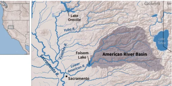
basin, considered to be one of the most important in the region because of its role in providing water fed by the melting snowpack of the Sierra Nevada to the central valley, covers an area of 1850 m2 and ends up in the confluence with the Sacramento River, 48 km after the Folsom reservoir. Downstream of the Folsom dam, there is the lake Natoma, which helps adjusting the dam’s regulations and fluctuations as a consequence of daily operations for power generation (Maher, 2008; U.S. Bureau of Reclamation, 2008).

Figure 3.4: Location of the American River Basin and Folsom Reservoir. Adapted from

Her-man and Giuliani (2018).

The dam’s storage capacity is of 977 thousand acre-foot (TAF), covering a surface area of 11,450 acres. It is the main storage and flood control point of the river, with its dam walls standing 427 m tall (Maher, 2008; U.S. Bureau of Recla-mation, 2008). The reservoir follows a historical operating strategies, mainly divided in two sections that varies according to the season: From November to February, which is the winter season, the conservation pool drops from 977 to 400 TAF, while the rest is used for flood control (Nayak et al., 2018). After that period, the flood pool decreases and the conservation pool equals the maxi-mum capacity at the beginning of the summer, as shown in Figure 3.5. More recently, an update was taken on the flood control policy, allowing for a smaller flood pool of 375 TAF, because the system got updated and is now benefiting from a short-term streamflow forecast, which enabled the anticipation from one to five days of the inflow (U.S. Army Corp of Engineers and U.S. Bureau of Recla-mation and California Department of Water Resources and H. I. Consulting, 2017). For a better understanding, Figure 3.6 depicts the historical release of water per each day of the year from 1995 to 2016 and the mean daily values, which

(47)

3.2. Folsom reservoir

are used as the daily demands value in this work. The release policy show a clear increase in demand during the irrigation period in California, the time of the year in which most of the water is used for agricultural supply, since there is no rain during this period and it is when the crops need it most to be able to grow. This policy, although recently updated, is likely to suffer from a decrease in performance, as the higher temperature in the future will provoke a decrease of the snowpack volumes and an earlier melting of the snow on the mountain range, deeply affecting the pattern of inflows of water into the reservoir (U.S. Bureau of Reclamation, 2008).

Figure 3.5: Historical rule curve of the Folsom reservoir. During winter the conservation pool

(48)

Figure 3.6: Historical register of release of water per day. Adapted from Herman and Giuliani

(2018).

One relevant characteristic of the Folsom reservoir is that it had release ca-pacity limitations. Nowadays, while its maximum release caca-pacity is about 34,000 cubic feet per second (cfs) through the regular outlets, when the level of water reaches the spillway, the release can grow up to 115,000 cfs. In case of extreme floods, there are three emergency spillway gates that allow for a total release of 160,000 cfs for a limited amount of time (U.S. Army Corp of Engineers and U.S. Bureau of Reclamation and California Department of Water Resources and H. I. Consulting, 2017). The channel was also improved, with its levees reinforced, guaranteeing 160000 cfs of discharge capacity (Maher, 2008).

The dynamics of the Folsom reservoir are modeled by a mass balance equa-tion of the water storage using a daily timestep, i.e.:

(49)

3.3. Data collection

where the variables s, r and q stand for storage, release and inflow, respec-tively. The multipurpose operations of the dam, targeting water supply and ensuring flood control, is modeled by means of the following objective func-tion: J = 1 H H

∑

t=0 max(Dt−rt+1, 0)2+ H

∑

t=0 c∗max(rt+1−rmax, 0)2 (3.2)

In this case, rt+1is the total release of water (including spills and constraints),

rmax is the limit to a safe release, which for this work is rmax =130, 000 cfs and

c = 1000 and represents a constant to make any flood event so costly that the evolutionary algorithm is expected to automatically avoid any case of flood. Therefore, this equation aims at reducing J by minimizing the deficits of water, especially large ones, since it is a quadratic function, while preventing releases above the limit to persist. In the case a final policy does result in a release value above the limit, it needs to be examined, as it implies that in the given sce-nario avoiding flood events is impossible, since all experimented solutions still suffered from flood events.

3.3 Data collection

The standard procedure for a long-term simulation of climate change requires both Representative Concentration Pathways (RCPs) and General Circulating Models (GCMs). Whilst the GCMs provide the proper mechanisms to process the climate along the years, the RCPs are entitled to guide the models through a pathway towards a specific target, providing all the information required. Naturally, different RCPs will generate different results, even if the model is the same for all of them. Likewise, running different models for a single RCPs will generate different results as well. In addition, for impact assessment, it is usual to downscale the GCM to a RCM so local results can be more reliable, as described in the previous subsection.

The data set used in this study includes 97 climate change scenarios of Fol-som reservoir inflows over the time horizon from 2000 to 2100. These projec-tions are the result of the combination of 31 GCM models with all four Repre-sentative Concentration Pathway (RCPs). Figure 3.1 provides further informa-tion on the models and their centres.