Universit`
a degli Studi di Pisa
Master thesis
Beware of topology! An analysis of
contagion in banking networks
Supervisors Candidate
Prof. Giorgio Fagiolo Dott. Matteo Benetton
Prof. Giulio Bottazzi
Contents
Acknowledgements 2
1 Introduction 3
2 Literature review 5
3 The basic model 13
4 The role of the interbank network structure 22
4.1 Capitalization and contagion . . . 22
4.2 Size of interbank exposure and contagion . . . 27
4.3 Connectivity and contagion . . . 30
5 Funding shock 35
5.1 Liquidity and contagion . . . 35
5.2 Connectivity and contagion . . . 37
6 Moving closer to real banking networks 41
6.1 Credit shock . . . 41
6.2 Funding shock . . . 43
7 Conclusions 46
References 50
Acknowledgement
I would like to express my deep and sincere gratitute to Professors Giorgio Fagiolo and Giulio Bottazzi. Their precious advice on how to do research in a rigourous, innovative and open-minded way are a fund of knowledge and experience I will always carry with me. Working with them has been both a pleasure and a privilege.
I would like to take this opportunity to thank three professors that had a huge impact on my academic and personal life during these years at the Sant’Anna School of Advanced Studies. I am grateful to Professor Fabrizio Bulckaen, who supervised me as my tutor since my first day at the School. It is difficult to find the words to describe his kindness, willingness and devotion. I would like to thank Professor Guido Maria Rey, who taught me how to approach real eco-nomics problems by posing the right questions. I will never forget his enthusiasm and firmness when sharing his vast experience with us young scholars. Last but not least, I am grateful to Professor Giovanni Dosi. Both in formal lectures and conferences and in informal dinners I had the opportunity to appreciate his revolutionary point of view and discuss it vividly. Their teachings and their example have been a milestone not only for my academic path, but also for my experience and my personal growth at the School.
1
Introduction
“Letting Lehman fail basically brought the entire world capital market down” commented Paul Krugman in an interview in 2008. His words emphasize how interdipendencies between countries may amplify through feedback effects the impact of an initial shock and lead to a worldwide crisis. In modern economies, the daily movements of goods, services, people and money across borders link countries in a complex and adaptive network. Complex because it involves a cumbersome and intricate net of interconnections; adaptive because it changes through abrupt shifts or gradual adjustments as result of the interplay between agents’ decisions and shocks. These two characteristics are especially relevant for the analysis of financial networks, which have attracted the attention of policymakers, scholars and media because of their growing importance for the global economy. If financial linkages among agents and countries are welfare enhancing during normal times, they could turn out to be dangerous liaisons when things get worse (Dasgupta, 2004; Lenzu and Tedeschi, 2012). Moreover, from the recent rush on the stock markets we learnt how looking at single enti-ties as isolated can give an incomplete, and possibly misleading, impression of the overall robustness of the system (Haldane, 2009).
This work studies the impact of the interbank network structure and some of its properties on systemic risk. The crucial question is what kind of interbank network is more or less prone to systemic collapse. To contribute to the ongoing debate on this topic we adopt a static model of contagion, based on Nier et al. (2007), which we test on different interbank network architectures. We employ the Erdos-Renyi model as our benchmark and compare it with the small-world networks by Watts and Strogatz (1998) and the scale-free networks by Barabasi and Albert (1999). Moreover, we construct a directed network model which exhibits tiering and other properties (i.e. density, clustering, assortativity and average path length) closer to those of real banking networks. In our analysis
we consider systemic risk due to interlocking credit exposures. On the one
hand, we study financial contagion as “the large scale breakdown of financial intermediation due to domino effects of insolvency” (Boss et al., 2003). On the other hand, we model bank runs as liquidity hoarding by banks, which can cascade through the interbank network and generate systemic liquidity crisis
(Gai et al., 2011). We proceed by computing the probability and extent of contagion, which may follow a shock affecting a random or a targeted bank in the network. With numerical simulations we assess the role of connectivity, net worth and liquidity buffer on systemic risk.
This study is motivated by the need of understanding how the topology of linkages among agents, markets, institutions and countries could increase or decrease the emergence of systemic risk. Research along this way has been has been blessed by many authoritative authors (Caballero, 2010; Stiglitz, 2009; Schweitzer et al., 2009).
The essay is structured as follows. Section 2 gives a brief overview of the em-pirical and theoretical literature on networks application in financial economics. In section 3 we describe the reference model and its developments. Section 4 analyses the role of the interbank network structure on contagion. Section 5 introduces shocks to the liability side, while in section 6 we extend the analysis to a tiered banking system. Section 7 concludes.
2
Literature review
Network theory has in recent years been applied to the study of financial sys-tems. Financial intermediaries are heterogeneous decision makers and their mu-tual interactions can lead to externalities, among which systemic risk is probably the most relevant. The result of these interdependencies is a complex system, for the comprehension of which network theory provides powerful tools.
“A network is, in its simplest form, a collection of points joined together in pairs by lines. In the jargon of the field the points are referred to as vertices or nodes” (Newman, 2010). Banking systems can be represented as a network, in which financial intermediaries are nodes and loans are weighted directed links between the counterparties. We can divide applications of network analysis to the financial sector into two broad categories.
The first stream of research is empirical and relies on the main results of graph theory to deal with the characteristics and the evolution of topology over time. Complex systems are analysed by means of the statistical properties of centrality, homophily and clustering indicators (for comprehensive reviews see Newman (2010), Goyal (2009), chapter 2 and Jackson (2008), chapter 2). The value added of a network analysis is that it is able to capture higher-order inter-actions and effects and to provide a system-wide view, that standard approaches cannot include. Methods and models are being developed in this area at a fu-rious pace, with contributions coming from a wide spectrum of disciplines. In economics many studies have applied these methods to the analysis of empirical networks, such as financial cross border exposures (among others Minoiu and Reyes (2011); Von Peter (2007); Garratt et al. (2011)) and national interbank
markets (among others Boss et al. (2003); Soram¨aki et al. (2007); Bech and
Atalay (2010)).
The knowledge of real banking systems is very important to make theoretical network models plausible, although rough, caricatures of reality. National bank-ing systems may vary from country to country. For example the Netherlands and Sweden have more concentrated banking systems, while Germany and Italy show lower concentration (Nier et al., 2007). Nothwistanding country-specific characteristics, studies of empirical banking systems provide some common ev-idences on their statistical properties.
Banking systems are organized in communities and display a tiered
struc-ture (Soram¨aki et al., 2007; Craig and Von Peter, 2010). Banking
net-works have usually a core-periphery structure, with a small number of large banks borrowing from a large number of small creditors. (Gai and Kapadia, 2010; Ladley, 2011; Haldane and May, 2011; May and Arinam-inpathy, 2010; Li et al., 2010; Lenzu and Tedeschi, 2012; Fricke and Lux, 2012). According to Bech and Atalay (2010) this small-bank-large-bank dichotomy is due to the fact that large banks are less risk averse, because they have more available options for obtaining necessary reserves. The correlation between the degree of node and the degree of its neighbours reveals a disassortative network, namely high-degree banks are likely to be more linked with lower-degree banks, and conversely (May and
Arinam-inpathy, 2010; Bech and Atalay, 2010; Soram¨aki et al., 2007). However,
Bech and Atalay (2010) note that disassortativity is lower when weighting by the value of links and, since high-degree banks are more likely to be associated with large-value links, this can suggest that even if small banks do not interact with small banks, large banks do interact with other large banks. A similar behaviour is at the basis of Craig and Von Peter (2010) model of interbank tiering. Top-tier banks lend to each other, while lower-tier banks do not.
Both Soram¨aki et al. (2007) and Bech and Atalay (2010) find very low connectivity, when studying the Fedwire and the Federal Funds networks, respectively. In both studies the density (i.e. the number of active links relative to the number of all possible links) is below 1%. Craig and Von Pe-ter (2010) study the German banking system and find that the network is sparse, with a density around 0.41% of possible links.
The average distance from a node to any other node (known as average path length) is usually low. Banking networks resemble small-worlds with
about 2-3 degrees of separation (Boss et al., 2003; Soram¨aki et al., 2007).
Low connectivity together with low distance enforce the idea of a net-work comprised of a core of interconnected hubs with whom the periphery interacts.
The degree is the number of connections a node has. The out-degree is the number of counterparties the bank lends to, while the in-degree is the number of counterparties the bank borrows from. Degree distributions of real banking systems have usually fat tails and follow power-law with
coefficient around 2 (Boss et al., 2003; Soram¨aki et al., 2007). Most banks
keep only few connections, while a small number of hubs, playing the role of intermediaries, have much higher degree. Bech and Atalay (2010) distinguish between the distribution of out-degree, which can be best fitted by a power law, and of in-degree, which is closer to a negative binomial. Soram¨aki et al. (2007) study also the weight of links and the node strength
( i.e. the sum of the weights of all links attached to it). Both follow a power law when weighted by the volume of payments and are closer to a lognor-mal when weighted by the value of payments. Bech and Atalay (2010) too find that node strength defined by the value sent or received, follows a log-normal distribution. These results are in line with the observed sig-nificant distribution in bank sizes (May and Arinaminpathy, 2010; Boss et al., 2003; Lenzu and Tedeschi, 2012). Moreover, strength is higher in banks belonging to the core and increase faster than the degree.
The clustering coefficient, which measure the probability that two neigh-bours of a node are neighneigh-bours themselves, is found to be low by Boss et al. (2003) and Bech and Atalay (2010). This can be due to the cost involved in keeping active links. High dispersion in the clustering across nodes and high clustering if nodes with lower degree are ignored is found
by Soram¨aki et al. (2007).
These characteristics will be useful to contruct and test a network model, able to explain some emerging phenomena of real interbank networks.
The second stream of research is mainly theoretical and addresses the key issues of systemic risk and financial stability, by modelling the financial system as a network among banks. The aim is to provide insights on how contagion dynamics function and transmit throughout the system. Four main categories of systemic risk have been identified by the literature (Allen et al., 2010; Gai
and Kapadia, 2010; Gai et al., 2011; Battiston et al., 2011; Georg, 2011; Nier et al., 2007; Ladley, 2011; Haldane and May, 2011; May and Arinaminpathy, 2010; Acharya and Yorulmazer, 2008).
Direct exposures between banks. In this category we can include both credit shock (i.e. a counterparty fails and does not repay the loan) and funding shock (i.e. a lender does not roll-over or even withdraws the loan). The former is at the basis of financial contagion and has a direct impact to the assets side; the latter phenomenon may cause bank run and affects directly the liability side.
Liquidity shock. “Fire selling” of assets and falling prices are the result of an idiosyncratic shock affecting even far away players in the system. This small initial shock has an impact that is greater the more correlated the portfolios of banks. A distinction can be made between strong liquid-ity shocks, associated with discounting specific assest classes, and weak liquidity shocks, which can be seen as a more general loss of confidence. Common shock. This channel is put forward by the view that financial
crisis are not random events, but an inherent part of the business cycle. A large shock leading to a fall of real estate or stock market prices can threat the stability of the whole system.
Information contagion. Poor performances or bad news about a bank may raise borrowing cost for the other banks in the network.
These channels are very likely to interact and reinforce each other during a crisis. Therefore, it is often not easy to distinguish among them. However, we will focus mostly on the interbank channel, because of its dual nature (Upper, 2010). On the one hand, interbank lendings represent a mechanism to absorb shocks, such as losses on activities or deposits withdrawals. On the other hand, interbank linkages are channels by which problems affecting one bank can spread to its neighbours and beyond, thus infecting the economy at large (Dasgupta,
2004). The debate about contagion through interbank claims goes back to
the work by Allen and Gale (2000), that deals with the trade-off between risk sharing versus financial fragility. They find a non-monotonic relation between
completeness of markets (as proxied by connectivity) and extent of financial crisis. In complete banking system the impact of an idiosyncratic shock becomes
negligible, since it is spread among many counterparties. On the contrary,
in incomplete system larger spillovers allow contagion to spread through the
network of interconnections. Moreover, they recognize that although
cross-bank linkages are useful for reallocating liquidity within the system, they cannot increase the overall available amount. Since their cutting-edge work, the use of network theory allowed many studies to bring the analysis of contagion in a complex system, able to account for direct and indirect channels.
Gai and Kapadia (2010) use a Poisson random graph and stylized banks’ bal-ance sheets to study the properties of financial systems affected by idiosyncratic and aggregate shocks. They show that financial systems have a “robust-yet-fragile” tendency, i.e. while the probability of contagion may be low, its effects can be extremely widespread. Increasing connectivity has a non-monotonic ef-fect on the probability of contagion, as in Allen and Gale (2000). Moreover, reductions in banks’ capital buffers both increase the probability of contagion for a given level of connectivity and widens the contagion window (i.e. the in-terval of connectivity level in which contagion may occurs). Gai et al. (2011) enrich the previous analysis and study contagion as a freeze in the interbank market due to liquidity hoarding by banks (a behaviour which has been widely observed during the current crisis). They found that more concentration in the banking sector, modelled drawing from a geometric distribution, make the sys-tem more robust to random shocks, but more susceptible to syssys-temic liquidity crisis and to targeted shocks. Moreover, they show that tougher liquidity re-quirements and even more targeted liquidity rere-quirements for systemic banks make the system less prone to contagion. Nier et al. (2007) build up a model of the banking system based on stylized balance sheets and on a given structure of interconnections. They perform numerical simulations, shocking one bank at a time, and show that contagion is a non-monotonic function of bank capi-talization and connectivity; that increase in the percentage of interbank assets increase the transmission of the shock; and that more concentrated networks tend to be more vulnerable to systemic risk. We will use the Nier et al. (2007) model as our benchmark, because it can be easily extended to more realistic
banking networks. Furthermore, their trasmission mechanism provides a clear and meaningful description of contagion, nothwistanding its simplicity. May and Arinaminpathy (2010) provide clear analytic approximations of the models by Gai and Kapadia (2010) and Nier et al. (2007) and enrich their analysis by adding a realistic mechanism of propagation of liquity shocks. They claim that homogeneity, which can be good from an individual perspective, can be destabilizing for the system as a whole.
Other recent works develop dynamic models of banking systems and study both the resilience of the network to financial distress and the endogenous build-up of systemic risk. Iori et al. (2006) study the role of interbank lending in ho-mogeneous and heterogeneous banking systems. In the former case, increasing connectivity always contribute to stabilize the system; in the latter case, this is true up to some point, but then higher connectivity leads to avalanches. In their model, contagion effects are due both to the knock-on from a failing bank to its direct creditors and to the increasing criticality in the system as a whole. Georg (2011) develops a dynamic model of a banking system with a central bank and analyze sistemic risk through contagion effect under three different classes of networks (random, small-world and scale-free). Beyond confirming previous results about the non-monotonicity between connectivity and conta-gion, the paper shows that scale-free networks are more robust than small-world networks, which in turn tend to be more stable than random networks. More-over, the “topology effect” tend to be larger during crisis time in all networks considered. The paper claims that both the topology and the level of intercon-nectedness affect the knife-edge property of interbank markets and compare the effects of common shocks, which pose greater threat to financial stability, and contagion, that has a stronger impact on liquidity volume. Ladley (2011) builds a model of the behavior of heterogeneous banks in a closed economy and study contagion due to small and system-wide shocks in different interbank market architectures. For single bankruptcies and small shocks, more connected inter-bank markets reduce the susceptability to contagion, by spreading the impact of failures; for larger shocks, higher interconnectivity results in more banks be-ing affected and failbe-ing. These results confirm the intuitions by Allen and Gale (2000). Therefore, there is no unique optimal level of connectivity, but it is
dependent on the shock severity. Ladley (2011) tests also the role of capital requirements and minimum reserve ratios. The overall effect of these measures is ambiguous, because they reduce bankruptcies, but at the same time reduce also lendings. Lenzu and Tedeschi (2012) study the resilience of the system and the emergence of systemic risk with a model of endogenous link formation, based on preferential attachments. Their surprising result, if compared with the works we mentioned previously, is that the scale-free network turns out to be more vulnerable to random attacks than the Poisson graph. According to the authors, this result is due to the fact that both the network topology and the heterogeneity among market partecipants play a role in shaping the robustness of the system.
Our work falls into the stream of theoretical literature that analyse contagion in exogenously given and fixed network stuctures. As emphasized by May and Arinaminpathy (2010) and Gai and Kapadia (2010), a static framework cannot capture the complexity of banks’ behaviours and feedback effects as contagion ripples through the system. However, contagion may spread very rapidly, giv-ing no time to banks for adoptgiv-ing countermeasures (Gai and Kapadia, 2010; Battiston et al., 2011). Moreover, our main aim is to analyze and compare the incidence of systemic risk in different banking system architectures. Therefore, our static balance sheet approach can provide a powerful tool of analysis.
Starting from our main reference (Nier et al., 2007) we move forward in two directions. On the one hand, we study contagion in a similar set-up, but adopt-ing network models that are closer to real interbank networks. Most studies are indeed limited to simulations assuming a random network (May and Ari-naminpathy, 2010), while it is of great importance to undertand (and test) the structure of real banking systems (Li et al., 2010). In particular we analyse the Watts and Strogatz (1998) small-world model, that is able to explain the low average path length and high clustering, and the Barabasi and Albert (1999) scale-free network, that is also able to reproduce power-law degree distributions. Both models display some properties in terms of path length, clustering and de-gree ditribution (in the case of the scale-free network), that are observed in real banking networks and cannot be generated by an Erdos-Renyi model. With
this analysis, we want to contribute to the open debate about the resiliency of different network models (Gai et al., 2011; Georg, 2011; Lenzu and Tedeschi, 2012). On the other hand, we adopt a comprehensive approach, which captures problems both on the assets side (credit shock) and the liabilities side (funding shock). Therefore, we can study contagion as a chain of multiple defaults due to transmission of losses through interbank exposures (Nier et al., 2007), and as a liquidity shortage due to the propagation of withdrawals via interbank linkages (Gai et al., 2011). Moreover, we can test both the role of capital and liquidity buffers on the stability of the system. Following Craig and Von Peter (2010), Fricke and Lux (2012) and Li et al. (2010) we will develop a tiered structure that is able to generate the emerging features of real banking networks we have seen previously. Eventually we will test the robustness of this closer-to-reality banking system.
3
The basic model
In order to build our banking system we refer to Nier et al. (2007) and mention explicitely any departures from or innovations to the basic set-up.
Banks’ balance sheets are composed by external and interbank assets, on the assets side, and net worth, customer deposits and interbank borrowing on the liability side. The condition for the bank j to be solvent is:
cj= (ej+ ij) − (dj+ bj) ≥ 0 (1)
where cj is the bank net worth, ej are external assets, ij interbank assets, bj
interbank borrowing and dj customer deposits. The solvency condition requires
that assets exceed liabilities that is equal to say that net worth is positive. As in Nier et al. (2007) the system in our benchmark case can be entirely described by the following set of parameters (γ, θ, p, N, E). γ represents net worth as a percentage of total assets, θ the percentage of interbank assets in total assets, p the probability of any two nodes being connected, N the number of banks and E the size of aggregate external assets of the banking system. The interbank network is described by a directed graph, where each link represents a directional lending relationship between two nodes. In such a framework banks can be net lenders or borrowers in the interbank market, that is we can have
ij 6= bj. The graph is binary since the weight is the same across all links and is
equal to w = I/Z, where I is the aggregate size of the interbank market and Z is the total number of links. The robustness of the banking system is then assessed by studying contagion due to the idiosyncratic failure of a bank at a time. Nier et al. (2007) simulate an initial shock that wipes out a percentage of the external
assets of the bank: sj = perc×ej. If the shock is greater than the bank net worth
(sj> cj), the affected bank defaults and the residual loss is transmitted through
the interbank market. The upper bound for the residual loss that can be spread
is given by bank’s total borrowing on the interbank market (bj). If the loss is
greater than bank j interbank borrowings (i.e. sj− cj> bj), depositors bear the
residual loss. Then every counterparty receives a loss equal to (sj−cj)
zj , where zj
is the number of bank’s j creditors. When affected neighbours experience a loss greater than their net worth, they fail and spread contagion further.
We now turn to the innovative part of our work. First of all, we “move backwards” and model the banking system as a binary-undirected graph. Undi-rected means that the graph is symmetric (all links are reciprocated), so that we
end up having ij= bj ∀j. The equality between interbank borrowing and
lend-ing at bank level cast some doubts on the usefulness of the interbank market, unless we introduce a maturity structure. This assumption, although unrealis-tic, is twofold useful. On the one hand, we can see if the main results by Nier et al. (2007) continue to hold when there is no mismatching in banks’ positions on the interbank market. On the other hand, we can extend the analysis to consider network structure that are closer to actual banking systems. Following Georg (2011), we study two network models, that resemble more closely than the Erdos-Renyi network the characteristics of real banking systems: the Watts and Strogatz (1998) small-world model and the Barabasi and Albert (1999) scale-free network. Their topological structures are likely to affect their vulnerability to contagion in a way different from an Erdos-Renyi network. In a small-world model, the short average path length may imply that an initial shock spreads rapidly to the whole system. A fat-tailed network configuration is expected to be more resilient to random shocks than an Erdos-Renyi network, but more
vulnerable to targeted failures (Gai et al., 2011; Georg, 2011)1.
The Watts and Strogatz (1998) network is characterized by low average path length, high clustering and exponentially-decaying degree distribution. Almost all nodes have same the number of partners and deviations are very rare events. A small-world network can be obtained applying the algorithm proposed by Watts and Strogatz (1998). At the beginning N nodes are located on a ring, where each node is linked to r neighbors on the left and r neighbors on the right (the degree is k = 2r). Then all links of all nodes at distance 1 are deleted and rewired to another node, not currently linked and at the same distance, with a probability equal to p (rewiring probability). After having considered all links with nodes at distance up to r the process stops. As p increases there is a sudden decrease in average path length, while clustering remains very high.
The Barabasi and Albert (1999) model is able to reproduce Watts and Stro-gatz (1998) features and allows for equilibrium power-law distributions. Power
laws are ubiquitous in natural and social systems, as a signature of complex behavior and self-organization. Most economic variables tipically follow (quasi) power law distributions, among which firm size, wealth, income and connectiv-ity in financial networks. The Barabasi and Albert (1999) model starts at t = 0
with N0 nodes connected in a complete undirected graph. At any time a node
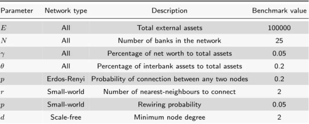
is added and connected to d distinct nodes among the pre-existing ones, each with probability proportional to its current degree. Both growth and preferen-tial attachments are essenpreferen-tial to reproduce power-law degree distributions. As noted by Georg (2011) and Lenzu and Tedeschi (2012) preferential attachments resemble the fact that few large and more interconnected banks are more trusted by other market participants and plays the role of central hubs in the network. Table 1 summarizes the structural parameters meaning and benchmark value.
(E, N, γ, θ, p) are as in Nier et al. (2007)2, while the benchmark parameters
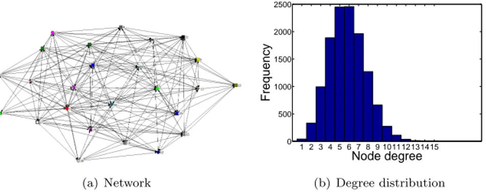
de-scribing the small-world and scale-free networks (r, p, d) are taken from Georg (2011). Figures 1, 2 and 3 show realizations of the networks with the benchmark
parameters and the degree distributions in 500 simulations3.
Table 1: Benchmark parameters
Parameter Network type Description Benchmark value
E All Total external assets 100000
N All Number of banks in the network 25
γ All Percentage of net worth to total assets 0.05
θ All Percentage of interbank assets to total assets 0.2
p Erdos-Renyi Probability of connection between any two nodes 0.2
r Small-world Number of nearest-neighbours to connect 2
p Small-world Rewiring probability 0.05
d Scale-free Minimum node degree 2
2A banking system comprising 25 banks is rather small. However, banking systems vary
greatly in size and we would like to stay as close as possible to our main reference, so that comparisons can be straightforward. Moreover, when dealing with our tiered model we will consider a more realistic network composed of 250 banks.
3As clearly pointed out by Soram¨aki et al. (2007) there are two classes of network formation
model. Equilibrium models have a fixed set of nodes with randomly chosen pairs of nodes connected by links (i.e. Erdos-Renyi). In non-equilibrium models the network grows by adding nodes and setting probabilities for links forming between new and existing nodes and between already existing nodes (i.e. scale-free). In this last case we take the stationary state of the network as our simulation platform.
(a) Network 1 2 3 4 5 6 7 8 9 101112131415 0 500 1000 1500 2000 2500 Node degree Frequency (b) Degree distribution Figure 1: Erdos-Renyi with N = 25 p = 0.2
(a) Network 1 2 3 4 5 6 7 0 2000 4000 6000 8000 10000 12000 Node degree Frequency (b) Degree distribution Figure 2: Small-world with N = 25 r = 2 p = 0.05
(a) Network 0 5 10 15 20 25 0 1000 2000 3000 4000 5000 6000 Node degree Frequency (b) Degree distribution Figure 3: Scale-free with N = 25 d = 2
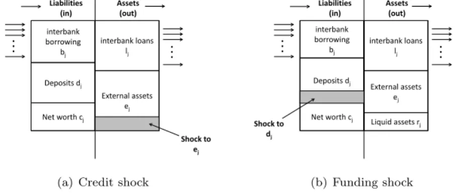
Our second improvement is to include in the Nier et al. (2007) model another type of systemic risk, which originates from a funding shock (Gai et al., 2011; Georg, 2011). In this case the bank receives a large deposits withdrawal to the liability side and starts hoarding liquidity in the interbank market. Therefore, other banks may experience gaps on the liability side of the balance sheet, so that liquidity shortages spread through the network via interbank linkages. Credit and funding shocks are represented in figures 4(a) and 4(b), respectively. As we have already noted, it is highly likely that financial contagion, following an idiosyncratic failure, goes hand in hand with bank run, consequent upon initial liquidity withdrawals. Net worth cj Deposits dj interbank borrowing bj interbank loans lj External assets ej Liabilities
(in) Assets (out)
Shock to ej
(a) Credit shock
Net worth cj Deposits dj interbank borrowing bj interbank loans lj External assets ej Liabilities
(in) Assets (out)
Liquid assets rj
Shock to dj
(b) Funding shock Figure 4: Balance sheet and shocks
When considering bank run we add to the asset side of banks’ balance sheet
liquid reserve, which represent a fixed percentage δ of total assets. In our
benchmark simulation we assume δ = 0.02 as in Gai et al. (2011). The condition for bank j to be liquid is:
rj = (dj+ bj+ cj) − (ej+ ij) ≥ 0 (2)
The liquidity condition simply requires that liquid reserves are positive. In this case the robustness of the banking system is judged by studying the prob-ability and extent of systemic hoarding due to the idiosyncratic run on a bank at a time. We assume a single bank receive an averse liquidity shock equal
to a percentage of its deposits: sj = perc × dj. If the shock is greater than
Morover, if the residual gap (after liquidity exhaustion) is greater than bank j
interbank loans (i.e. sj− rj> lj), it induces losses on external assets. As in Gai
et al. (2011) we assume that banks cannot raise any new deposits. Moreover, we compare the results when assuming full withdrawal (i.e lending banks withdraw their entire deposits irrespective of their own “liquidity shortfall”) and partial withdrawal (i.e. banks hoard only the amount they are short by). Banks try to cover the liquidity gap by withdrawing equally from all counterparties, which
therefore experience in turn a gap of (sj−rj)
zj , where zj is the number of banks
borrowing from bank’s j and sj− rjis at most equal to lj (i.e. bank j interbank
loans). When affected neighbours experience a withdrawal greater than their liquidity reserve, they become illiquid and the bank run spreads further.
In the last part of our work we develop a more realistic banking network and we test its robustness to the two types of contagion we have defined. As noted by Fricke and Lux (2012) “core-periphery structure could be seen as a new stylized fact of modern banking systems”. Therefore, we consider a tiered structure with a core (C) composed by large connected banks, a semi-periphery (SP) with medium banks and a periphery (P). To build the banking system we follow the approach by Craig and Von Peter (2010) and Fricke and Lux (2012), which recall the literature on generalized blockmodeling. Drawing ispiration from the empirical insights we have described before, regarding both network structures and economic rationale at the basis of the interbank market, we assume that:
1. Large banks are all interlinked among themselves. They borrow both from medium banks and small banks from the periphery, although to a different extent. Large bank also lend to medium and small banks, but they are net borrowers in the interbank markets, as shown by Bech and Atalay (2010) and Ladley (2011).
2. Medium banks belonging to the semiperiphery act as intermediaries be-tween the periphery and the core of the network. Their primary role is to borrow from small banks and redirect these resources to large banks at the center of the network. Only minor interactions take place between medium banks.
3. Small banks collect savings and lend them to medium and large banks. They also receive loans from higher-tier banks, but they end up usually as net lenders. Small banks do not interact among themselves.
Our banking system can be described by the following adjacency matrix4:
A = C − C C − SP C − P SP − C SP − SP SP − P P − C P − SP P − P = 1 RRc−sp RRc−p CRsp−c RRsp−sp RRsp−p CRp−c CRp−sp 0 = 1 4 × p 0.5 × p 2 × p 0.5 × p 0.5 × p 0.1 × p 0.1 × p 0 (3)
In the second matrix 1 is a complete block, 0 is a null block, CR is a
column-regular block, RR is a row-column-regular block5. By using row and column regular
blocks we place restrictions only on the core and the semiperiphery. Every bank belonging to the core must be connected to at least one bank in the semiperiphery and the periphery, but the converse not need to be true. In turn, every bank in the semiperiphery must be linked to at least one bank in the periphery and the converse need not hold.
In our simulation we assume the core to be composed of roughly 3% of banks as suggested by Craig and Von Peter (2010), while the semiperiphery is
composed of 10% of banks6. We define a reference probability to be linked p,
which is multiplied by a factor dependent on the block of the matrix (see matrix 3). In our benchmark case p = 0.1 and as p increases connectivity increases. All large banks are interlinked, while no interactions take place between small
4The element A
ijis 1 if bank i borrows from bank j and 0 otherwise. Therefore, the rows
of the matrix represent borrowings, while the columns lendings. The matrix is non-symmetric and binary. We leave the introduction of links’ magnitude for future works.
5A column-regular block has each column, but not necessarely each row, covered by at
least one 1. The opposite is true for a raw-regular block. All diagonal elements are set to 0, because no bank can lend to or borrow from itself.
6Fricke and Lux (2012) identifies a larger core consisting of roughly 25% of all banks,
studying the Italian interbank market. This result is probably driven by the very high density of above 20% that they find, compared to only 0.6% for the German market in Craig and Von Peter (2010). To the best of our knowledge there is no evidence and clear definition about the concept of semiperiphery. However, in our model the sum of large and medium banks represent nearly 15% of the system, which is consistent with the model by Ladley (2011).
banks. Medium banks lend to and borrow from about 5% of other medium banks. Large banks in the core are intermediaries, borrowing from and lending to both medium and small banks. Both large banks and medium banks borrow
from 5% and lend to 1% of small banks in the periphery7. Therefore, also banks
in the semiperiphery are intermediaries, but they differ from banks in the core, because they are less interconnected among themselves.
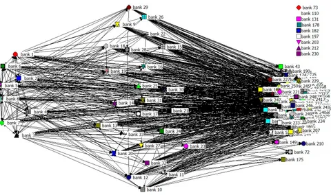
In figure 5 we plot the graph of our tiered network with 250 banks8.
Figure 5: Tiered network
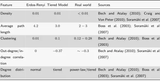
We run our model 500 times and compare its main features with those of an Erdos-renyi network of comparable size and with those we have found in the empirical literature. As we can see from table 2 our tiered banking network is able to reproduce many of the observed characteristics of real banking systems.
7This asymmetry is in line with Bech and Atalay (2010), Lenzu and Tedeschi (2012) and
Ladley (2011). These studies claim that few large borrowing banks attract a high percentage of incoming links. On the contrary, Fricke and Lux (2012) find that for core banks the out-degree exceeds the in-out-degree. Therefore, in their core-periphery model the density in the block of loans from the core to the periphery is higher than the density in the block defining core borrowings from the periphery.
8Although banking systems vary greatly in size, we can imagine a medium-sized banking
system to be composed of some 250 banks (Craig and Von Peter, 2010). Moreover, Gai et al. (2011) uses a network comprising 250 banks in their simulations.
Table 2: Tiered network with N = 250
Feature Erdos-Renyi Tiered Model Real world Sources
Density 0.01 0.01 < 0.01 Bech and Atalay (2010); Craig and
Von Peter (2010); Soram¨aki et al. (2007)
Average path
length
4.2 3.0 2 − 3 Boss et al. (2003); Soram¨aki et al.
(2007)
Clustering 0.01 0.1 0.12 − 0.28 Bech and Atalay (2010); Boss et al.
(2003)
Out-degree/in-degree correla-tion
0 −0.37 ∼ −0.3 Bech and Atalay (2010); Soram¨aki et al.
(2007)
Degree
distri-bution
normal tiered power-law/tiered Bech and Atalay (2010); Boss et al.
(2003); Soram¨aki et al. (2007)
Table 3 reports average total degree and net position of large, medium and small banks for different level of network connectivity. We can see that the structure in blocks is preserved as connectivity rises. Large banks in the core have more links than banks in the semiperiphery, which in turn have more connections than banks in the periphery. Moreover, banks in the core and in the semiperiphery end up as net borrowers, while small banks are on average net lenders. This structure with many small creditor banks and a few large borrowing banks is consistent with Bech and Atalay (2010), Lenzu and Tedeschi (2012) and Ladley (2011).
Table 3: Characteristics by tier
Connectivity p = 0 p = 0.1 p = 0.2 p = 0.3 p = 0.4 p = 0.5 p = 0.6 p = 0.7 p = 0.8
Average total degree
Large 14 42 70 94 111 129 142 155 168
Medium 0 20 41 60 76 93 109 124 139
Small 0 2 4 6 8 10 12 14 16
Average net position (out-degree − in-(out-degree)
Large 0 −14 −28 −36 −39 −43 −52 −61 −70
Medium 0 −7 −15 −23 −32 −43 −52 −61 −70
4
The role of the interbank network structure
In this section we show that the main results by Nier et al. (2007) are still valid if we consider an undirected graph. This means that the asymmetry in banks’ balance sheets between interbank assets and liabilities is not necessary to generate contagion. Therefore, we use a binary-undirected graph to model the interbank system. In this way we can extend the analysis to the two models we described previously, that are able to reproduce more closely stylized properties of real banking systems. At the same time, we bring forward the ongoing debate on the robustness of different financial architectures to idiosyncratic random and targeted shocks (Georg, 2011; Gai et al., 2011; Lenzu and Tedeschi, 2012), by comparing the Erdos-Renyi model with small-world and scale-free networks.In our simulations we take a realization of the random network and shock one bank at a time, by wiping out all its external assets. We perform several experiments letting the benchmark parameters vary and evaluate the robustness of different network architectures computing the average number of defaults. In the following subsections we analyse the role of capital, interbank assets and connectivity on the size of the default cascade.
4.1
Capitalization and contagion
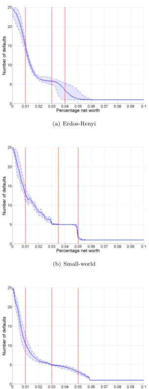
We first test the role of capital as a buffer against contagion, by varing the ratio of net worth to total assets (γ). The failure of the first bank affects through interbank lending connected banks. If the loss incurred is greater than the capital, the counterparty fails too and spread contagion further. Therefore, capital is a “shock-absorber” and the higher the net worth of a bank, the greater the ability of the bank to withstand external shocks. This result is evident from figures 6(a), 6(b) and 6(c).
In all network structures considered we observe a non-linear relation between contagion and bank capitalization. For level of net worth below 1% the default of a bank spreads throughout the whole system, because the lack of a sufficient capital buffer allows the initial failure to generate multiple rounds of defaults. In the Erdos-Renyi and small-world network a capital buffer at 5% of assets is enough to stop even the first round of contagion and only the shocked bank
(a) Erdos-Renyi
(b) Small-world
(c) Scale-free
defaults. In the case of the scale-free network a higher level of capitalization, around 6%, is required to limit default to the affected bank. The number of defaults in the small-world network is higher than in the other two for levels of net worth between 1 and 3%. Then it stabilizes to five in the interval 3-4.5%, before falling to 1 when net worth reaches 5%. In the scale-free network the effect of rising capital requirement is greater for low level of net worth, i.e. the number of defaults drops more quickly. Further increases in the percentage of net worth have a milder effect on reduncing the number of defaulting banks and we do not observe a second drop as in the Erdos-Renyi and small-world networks. Apart from small differences we can idenfity in all networks three main regimes: a first one characterized by low level of net worth and systemic contagion, an intermediate one where the number of defaults does not vary much with capital, and a final one where net worth is high enough to stop even the first round of contagion.
However, the analysis of the mean-behaviour does not tell the full story. Despite all networks show a similar relation between net worth and contagion, the distributions of defaults reveal some differences. We focus our analysis on the distribution of defaults for key levels of capital, which correspond to the red lines in figures 6(a), 6(b) and 6(c). In the case of the Erdos-Renyi network we see that there is not a typical scale. For low level of capitalization, γ = 1%, we have a sort of uniform distribution of defaults. As net-worth rises, the number of defaults converges to a normal distribution with a mean moving to the left.
The picture is different in the case of the scale-free network. For example,
when capital is at 3% of total assets we have an average number of defaults around 5 both in Erdos-Renyi and scale-free networks. However the former has an approximately normal distribution of defaults, while the latter distribution is more skewed to the right (see figures 7(b) and 9(b)). The distribution of defaults in the scale-free network shows a persistent right fat tail of defaults that is due to the heterogenity of the degree distribution. The distribution of defaults in the case of the small-world network appear always to be more picked, so that we can properly identify a characteristics scale of the cascade (figures 8(a), 8(b), 8(c)). This “representative cascade” moves to the left as the level of capitalization increases.
0 5 10 15 20 25 0 0.01 0.02 0.03 0.04 0.05 0.06 Number of defaults Relative frequency (a) γ = 1% 12 345678 9 10 11 12 13 14 0 0.05 0.1 0.15 0.2 Number of defaults Relative frequency (b) γ = 3% 1 2 3 4 5 6 7 8 910 11 12 0 0.05 0.1 0.15 0.2 0.25 Number of defaults Relative frequency (c) γ = 4% Figure 7: Erdos-Renyi 0 5 10 15 20 25 0 0.05 0.1 0.15 0.2 0.25 0.3 0.35 Number of defaults Relative frequency (a) γ = 1% 1 2 3 4 5 6 7 8 9 0 0.2 0.4 0.6 0.8 1 Number of defaults Relative frequency (b) γ = 3.5% 1 2 3 4 5 6 7 0 0.1 0.2 0.3 0.4 0.5 0.6 0.7 0.8 Number of defaults Relative frequency (c) γ = 5% Figure 8: Small-world 0 5 10 15 20 25 0 0.02 0.04 0.06 0.08 0.1 0.12 0.14 Number of defaults Relative frequency (a) γ = 1% 0 5 10 15 20 0 0.1 0.2 0.3 0.4 0.5 Number of defaults Relative frequency (b) γ = 3% 123456789 10 11 12 13 14 15 0 0.05 0.1 0.15 0.2 0.25 0.3 0.35 Number of defaults Relative frequency (c) γ = 5% Figure 9: Scale-free
The analysis of the distributions of defaults allows us to consider another question that has relevant policy implication. Without any doubt it is important to know the average number of defaults associated to a certain level of capital. However, to judge the stability of the system it will be even more important to study the probability that an initial failure will lead to a widespread contagion, that no external intervention can bailout. We define an event extreme when the initial failure lead to the default of at least 40% of the system (10 banks out of 25 in our case). Figure 10(a) shows the probability of at least 40% of the system failing for different level of capitalization in the three networks under analysis. For level of net worth below 2% the small-world network is the most fragile, while the scale-free is the most robust. The opposite is true for more capitalized systems. The Erdos-Renyi network lies in between the other two structure along all level of capitalization. We test the robustness of our results by considering an event extreme when 30% or 50% of the system fails. Despite some changes in the level of capitalization for which probabilities drop, the main results we have obtained are unaffected.
0 0.02 0.04 0.06 0.08 0.1 0 0.1 0.2 0.3 0.4 0.5 0.6 0.7 0.8 0.9 1
Percentage net worth
Probability of default 40% of the system
Erdos−Renyi Small−world Scale−free
(a) Extreme Events
0 0.02 0.04 0.06 0.08 0.1 0 5 10 15 20 25
Percentage net worth
Number of defaults Erdos−Renyi Targeted Erdos−Renyi All Small−world Targeted Small−world All Scale−free Targeted Scale−free All (b) Targeted shock Figure 10: Network Comparison
In figure 10(b) another relevant message can be read. We compare for dif-ferent level of capitalization the average number of defaults upon the failure of all banks (bechmark shock) with the contagion due to the failure of the most connected banks in the network (targeted shock). In a small-world network we do not observe a significant difference between the average case and the targeted shock and this is the natural consequence of higher homogeneity among banks. In this case a unique capital requirement can be an optimal policy, provided that
the appropriate level is found. The Erdos-Renyi network lies in between, while in the scale-free network we observe the greatest difference between the bench-mark case and the targeted shock. The latter involves one or more banks that are by far more connected than the average bank so that more counterparties are involved. The stronger impact of a targeted shock in a more concentrated network, as the scale-free, is in line with the findings of Gai et al. (2011).
4.2
Size of interbank exposure and contagion
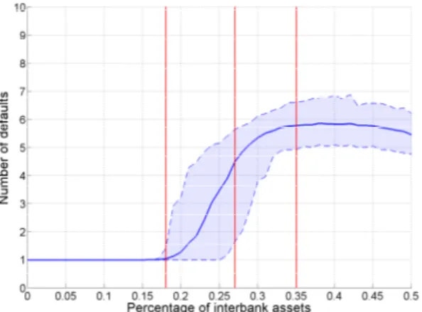
In this part we aim to understand what relation exists between the size of the interbank exposure in banks’ balance sheet and contagion. As in Nier et al. (2007) we increase the percentage of interbank asset in total assets (θ), keeping fixed the absolute size of external assets (E) and the mechanism governing the number of links. In this way an increase in interbank assets translates into an increase in the size of each interbank relationship, the weight of the link, and a raise in net worth, that by construction is a fixed proportion of total assets. An increase in the percentage of interbank assets has two opposite effects. On the one hand, increasing the magnitude of interconnections among banks raises the shock to interbank creditors itself; on the other hand, there is a parallel increase in net worth that dampens contagion effects.
In figure 11(a) we observe that the average number of default rise from 1 to 6 in an interval for θ between 20% to 30% and then stabilizes. A qualitative similar behaviour is observed in the small-world and scale-free networks, but with some remarks. We observe in figure 11(b) that the number of defaults in a small-world network jumps when θ is around 20% and continue to rise slightly thereafter. The average number of default for an interbank market covering 50% of assets is around 8, which is higher than in the case of a random or a scale-free network. In the latter, the average number of defaults begins to rise when θ is around 17%, but increasing further the size of interbank exposure does not raise much the number of defaults, that converges to 4 with θ around 50%.
This effect is in line with Gai et al. (2011), where an increase in complexity, proxied by unsecured interbank liabilities as percentage of banks’ balance sheet, raises the probability and extent of contagion. The small increase in the average
(a) Erdos-Renyi
(b) Small-world
(c) Scale-free
number of defaults, we found even for very high level of interbank exposure, is due to the rise in net worth that comes along with increasing assets size, dampening contagion. 1 2 3 4 5 6 7 0 0.2 0.4 0.6 0.8 1 Number of defaults Relative frequency (a) θ = 18% 1 23 4 5 67 8 9 10 11 12 13 0 0.05 0.1 0.15 0.2 Number of defaults Relative frequency (b) θ = 27% 1 23 4 5 67 8 9 10 11 12 0 0.05 0.1 0.15 0.2 Number of defaults Relative frequency (c) θ = 35% Figure 12: Erdos-Renyi 1 2 3 4 5 6 0 0.1 0.2 0.3 0.4 0.5 0.6 0.7 0.8 Number of defaults Relative frequency (a) θ = 20% 1 2 3 4 5 6 7 8 0 0.2 0.4 0.6 0.8 1 Number of defaults Relative frequency (b) θ = 30% 1 2 3 4 5 6 7 8 9 10 0 0.05 0.1 0.15 0.2 0.25 0.3 0.35 0.4 Number of defaults Relative frequency (c) θ = 45% Figure 13: Small-world 1 23 4 5 67 8 9 10 11 12 0 0.1 0.2 0.3 0.4 0.5 0.6 0.7 Number of defaults Relative frequency (a) θ = 18% 1 23 4 5 67 8 9 10 11 12 13 0 0.05 0.1 0.15 0.2 0.25 0.3 0.35 Number of defaults Relative frequency (b) θ = 25% 1 2 3 4 5 6 7 8 9 10 0 0.1 0.2 0.3 0.4 0.5 Number of defaults Relative frequency (c) θ = 40% Figure 14: Scale-free
Again the study of distributions of defaults reveal some interesting insights. For level of interbank assets close to the threshold when second-round defaults begin to appear, all networks have a mode in correspondence with only the first bank defaulting and tails of less likely multiple failures. As interbank activi-ties increase, the distribution of defaults in the Erdos-Renyi network converges to a normal with a mean moving to the right and stabilizing slightly above 5.
The distribution in the small-world network is right-skewed when the number of defaults jumps at θ around 20%, normal in correspondance with the plateau when θ is between 21 and 32%, and left-skewed when the number of defaults in-creases further. The scale-free network maintains its characteritics right-skewed distribution with fat-tails, as the percentage of interbank assets increases.
4.3
Connectivity and contagion
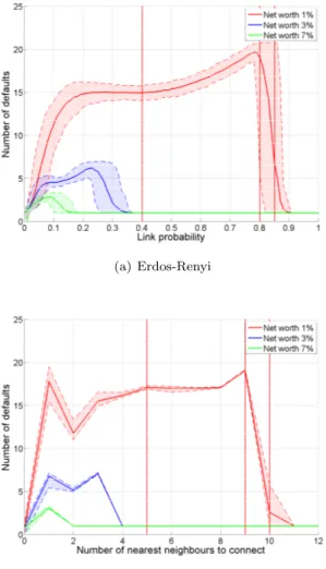
We now analyse the impact of the topology of the network on contagion, looking at different levels of connectivity and their interplay with net worth. As we have already seen in the literature review, interbank connections play a dual role, either as “shock-absorbers” or as “shock-transmitters”. The debate on which role prevails and under which conditions is ongoing.
Nier et al. (2007) find a non-monotonic effect of the degree of connectivity on contagion (see figure 15(a)). For low level of connectivity an increase in p leads to an increase in the number of defaults, because more banks can be hitten by subsequent rounds of the shock. Then rising connectivity may increase, decrease or not affect the number of defaults. Eventually, for high levels of p connec-tivity allows the shock to be spread among many counterparties, thus reducing contagion. The level of connectivity interacts with the level of capitalization of the banking system in determining its robustness. In better capitalized systems, connections are more likely to act as “shock-absorbers”, while the opposite is true when the system is undercapitalized.
In figures 15(b) and 15(c) we extend the analysis to small-world and scale-free networks, respectively. The results for the small-world network resemble those we observed for the random network. As the number of neareast-neighbours to connect increases, the number of defaults first increases, then stabilizes or diminishes, before raising again and eventually falling for higher levels of con-nectivity. The interplay between connectivity and capitalization is as expected. In highly capitalized systems, with a net worth to total assets of 7%, connectiv-ity acts to stabilize the system even when the degree is just 4. When the system is under-capitalized, connectivity raises the potential for the shock to spread for a wide interval of nearest-neighbours.
(a) Erdos-Renyi
(b) Small-world
(c) Scale-free
network. The M-shape relation between connectivity and number of defaults disappears and the interaction between connectivity and capitalization plays an even stronger role for the stability of the system. The number of defaults rises steadely with connectivity until a maximum and then starts to diminish. In the scale-free we do not observe an intermediate zone of connectivity in which the average number of default is stable. Interbank connections act exclusively as “shock-transmitters” until the network becomes “dense enough”.
We now take a closer look at the distributions of the number of defaults in the undercapitalized scenario (i.e. γ = 1%). In the Erdos-Renyi network the number of defaults is stable around 15 for a wide range of intermediate level of connectivity. However, the average does not allow to understand properly what happens. The number of defaults have a bimodal distribution with the global maximum in correspondance with all the system collapsing and a local maximum when 9 banks default. When 80% of possible links are active, we observe a left-skewed normal distribution with an average just below 20. Further increase in connectivity, increase system resilience, as we can see from the drop in the average number of defaults due to contagion. With a connectivity of 85% the default of only the shocked bank becomes the most likely event, although we can rarely observe widespread contagion.
The small-world network shows always a typical scale, as expected. In the plateau corresponding with intermediate level of connectivity, the distribution is normal and has a pick when 17 banks default. When the average degree is 18, we have the highest average number of defaults and a nearly degenerate ditribution with mode when the contagion of a bank affects all its neighbour (i.e. a total of 19 banks fail). With a further increase in connectivity, links turn from “shock-spreaders” to “shock-absorbers”. When the average degree is 20, no contagion occurs in more than 90% of the simulations, but when it occurs it involves all neighbours. The small-world network display the “robust-yet-fragile” property, which was found in previous studies (Gai and Kapadia, 2010; Gai et al., 2011).
The distribution of defaults in the scale-free network for low level of con-nectivity is bimodal, with extreme scenarios having a higher probability than intermediate contagion. As connectivity increases, the probability mass shifts
from events where contagion remains local to more systemic scenarios. In cor-respondence with the highest average number of default, the distribution of defaults approximates a left-skewed normal distribution, as was the case for the Erdos-Renyi network. Increasing connectivity the distribution of defaults becomes normal and centered around 5. The major difference of the scale-free network with respect to the previous two is that when connectivity is high enough the scale-free does not allow for systemic crisis (as can be seen from figure 25(c) contagion never involves more than 10 banks). This result is at odd with the one by Gai et al. (2011), who find more concentrated networks to be more susceptible to systemic crisis. However, no hasty conclusion should be taken. As a matter of fact, the absence of systemic crisis in scale-free net-works is observed for very high level of connectivity, while we have seen that
real world banking systems tend to be sparse (Soram¨aki et al., 2007; Bech and
Atalay, 2010; Craig and Von Peter, 2010)9.
0 5 10 15 20 25 0 0.02 0.04 0.06 0.08 0.1 0.12 0.14 Number of defaults Relative frequency (a) p = 0.4 0 5 10 15 20 25 0 0.05 0.1 0.15 0.2 Number of defaults Relative frequency (b) p = 0.8 0 5 10 15 20 25 0 0.05 0.1 0.15 0.2 0.25 0.3 0.35 Number of defaults Relative frequency (c) p = 0.85 Figure 16: Erdos-Renyi 0 5 10 15 20 25 0 0.1 0.2 0.3 0.4 0.5 0.6 0.7 Number of defaults Relative frequency (a) r = 6 0 5 10 15 20 25 0 0.2 0.4 0.6 0.8 1 Number of defaults Relative frequency (b) r = 10 0 5 10 15 20 25 0 0.2 0.4 0.6 0.8 1 Number of defaults Relative frequency (c) r = 11 Figure 17: Small-world
9Further simulations are needed to study more deeply the role of connectivity under
differ-ent topologies. For example, it could be interesting to introduce targeted shocks and stress-test banking networks of different sizes.
0 5 10 15 20 25 0 0.05 0.1 0.15 0.2 0.25 Number of defaults Relative frequency (a) d = 5 0 5 10 15 20 25 0 0.05 0.1 0.15 0.2 Number of defaults Relative frequency (b) d = 14 1 2 3 4 5 6 7 8 9 10 0 0.05 0.1 0.15 0.2 0.25 Number of defaults Relative frequency (c) d = 15 Figure 18: Scale-free
5
Funding shock
In this section we extend the Nier et al. (2007) model to study bank run. Banks running on other banks is an important feature of modern financial sys-tem, which can lead to system-wide liquidity collapse (Gai et al., 2011).
In our simulations we take a realization of the random network and shock
one bank at a time, by wiping out 50% of its deposits (dj in figure 4(b)). The
two extreme cases of full withdrawal and partial withdrawal are shown. So that we can imagine reality to be somewhere in between. In the following subsections we analyse the role of liquid reserve and connectivity on the size of the hoarding cascade.
5.1
Liquidity and contagion
The role of liquidity regulation is analyzed by varying the parameter δ, which represents the percentage of liquid reserves to total assets. In this section we focus on scale-free networks, which are better approximation of real-world bank-ing systems (Gai et al., 2011; Craig and Von Peter, 2010; Lenzu and Tedeschi, 2012). From figure 19 we observe a decrease in the size of contagion, as liquid reserve increase. For percentages of liquid reserves below 5.5% huge differences can be seen between the two extreme cases of partial and full withdrawal. In the former, the introduction of even small percentage amount of liquid reserves leads to a significant drop of the size of the hoarding cascade. The effect of liquid reserves as buffer is in this case reinforced by the attenuation mechanism, that is given by the fact that banks’ liquidity shortfalls are the only determinant of the amount of hoarding. With liquid reserves between 1% and 3.5%, usually banks affected in the first-round start hoarding in turn. Liquid reserves above 5% are on average enough to withstand an initial run of 50% of deposits even to the most connected bank. When banks withdraw their entire interbank lending irrespective of their own liquidity gap, as in Gai et al. (2011), things change a lot. Liquid reserves become “useful” to keep down systemic liquidity shortages, only when the ratio is above 3.5%. No attenuation mechanism is in place here. When liquidity is between 3.5% and 5.5% we observe a steady drop in the size of the hording cascade, until all neighbors of the shocked bank are able to cover
the gap with their own reserves.
Figure 19: Liquid reserve and contagion in a scale-free network
We now turn to the analysis of the distributions of hoarding banks for key level of liquid reserve (see figures 20 and 21). In the case of partial withdrawal, the distribution of hoarding banks is always right-skewed, recalling the distri-bution of degrees in scale-free networks. Moreover, as δ rises the distridistri-bution moves to the left and its support becomes less broad. When full withdrawal is assumed the distribution is splitted into the two extreme cases of systemic and local hoarding. For level level of liquid reserve at 4% or below, in nearly 95% of the cases all the banking system suffers from liquidity shortages. When δ is around 0.48% systemic contagion still remains the most likely event, while a right-skewed distribution in cases of local contagion begins to emerge. As liquid reserves rise further, the probability mass moves to the left, i.e. cases of no hoarding or first-round hoarding become more likely. With δ around 5% the extreme scenario of systemic liquidity shortages remain a possible, altough less likely, event.
The higher incidence of systemic liquidity shortages in the case of full with-drawal is no surprise. What is more interesting is to note that when no atten-uation effect is in place the system has a unique “tipping-point” and for level of liquid reserve above 5% display the “robust-yet-fragile” tendency observed by Gai and Kapadia (2010) and Gai et al. (2011). With partial withdrawals, intermediate regimes can be identified and the distribution of defaults seem to
0 5 10 15 20 0 0.05 0.1 0.15 0.2 0.25 0.3 0.35 0.4
Number of hoarding banks
Relative frequency (a) δ = 1% 1 23 4 5 67 8 9 10 11 12 0 0.1 0.2 0.3 0.4 0.5
Number of hoarding banks
Relative frequency (b) δ = 3% 1 2 3 4 5 6 7 0 0.1 0.2 0.3 0.4 0.5
Number of hoarding banks
Relative frequency
(c) δ = 5% Figure 20: Scale-free: partial withdrawal
0 5 10 15 20 25 30 0 0.2 0.4 0.6 0.8 1
Number of hoarding banks
Relative frequency (a) δ = 4% 0 5 10 15 20 25 30 0 0.1 0.2 0.3 0.4 0.5 0.6 0.7
Number of hoarding banks
Relative frequency (b) δ = 4.8% 0 5 10 15 20 25 30 0 0.1 0.2 0.3 0.4 0.5 0.6 0.7
Number of hoarding banks
Relative frequency
(c) δ = 5.5% Figure 21: Scale-free: full withdrawal
be closer to the degree distribution.
5.2
Connectivity and contagion
In this part we study under different network topologies the role of connectiv-ity in enhancing or dampening liquidconnectiv-ity hoarding. As with financial contagion, interbank connections can act as “shock-absorbers” or as “shock-transmitters” in the case of a bank run. Therefore, we compare the role of market complete-ness in the two cases contagion may take place. Moreover, we consider the relationship between connectivity and size of contagion in the extreme case of full withdrawal.
Looking at figure 22 and 23 we can note a clear difference with respect to the case of financial contagion upon idiosyncratic default (see figures 15(a) and 15(b)). In both Erdos-Renyi and small-world networks the number of hoarding banks increase steadily as connectivity rises, until it drops when the system becomes almost complete. We do not observe, as with financial contagion, and immediate jump in the number of affected banks and a plateau for a wide range of intermediate levels of connectivity. The relation between connectivity and size of contagion in the scale-free network is similar irrespective of the origin of
(a) Partial withdrawal (b) Full withdrawal Figure 22: Erdos-Renyi
(a) Partial withdrawal (b) Full withdrawal
Figure 23: Small-world
(a) Partial withdrawal (b) Full withdrawal
Figure 24: Scale-free Connectivity and contagion
the shock. However, the number of defaulting banks increases faster for low level of connectivity and then the speed of growth slows down. The maximum size of contagion is when the minimum node degree d is 14. With funding shocks, the number of hoarding banks first increases, then falls and eventually rises again until a peak for the same level of connectivity observed in the credit shock case. When liquidity is abundant, connections are more likely to act as “shock-absorbers”, while the opposite is true when liquidity is scarse. It is interesting to note that in all topologies there seem to exist a level of connectivity for which the percentage of liquid reserves matters less, i.e. the size of the bank run is the same irrespective of the available liquidity. At such point we have only first round defaults both with liquid reserves at 1% and 3%. Further rises in connectivity imply a dichotomy between more liquid systems, where connectivity spreads the shock enough to be limited to the affected bank, an less liquid ones, where more linkages lead to higher contagion rounds. A pro-connectivity view must take this insight carefully into account.
On the right side of figures 22, 23 and 24 we analyze the role of connectiv-ity when illiquid banks withdraw all loans in the interbank market. The mere existence of an interbank network lead to systemic hoarding behaviour, which involves all banks. Further increases in connectivity allow to stabilize the sys-tem together with an appropriate level of liquid reserves. If liquidity is scarse, systemic liquidity crisis can be the rule even for high level of connectivity. Such results confirm the original intuition by Allen and Gale (2000), that connected but incomplete markets are more exposed to systemic risk than complete market or disconnected ones. Moreover, the scale-free network becomes more robust for lower level of connectivity than the Erdos-Renyi and small-world network.
0 5 10 15 20 25 0 0.05 0.1 0.15 0.2 0.25 0.3 0.35 0.4
Number of hoarding banks
Relative frequency (a) d = 2 0 5 10 15 20 25 30 0 0.05 0.1 0.15 0.2
Number of hoarding banks
Relative frequency (b) d = 14 0 5 10 15 20 25 0 0.02 0.04 0.06 0.08 0.1 0.12 0.14 0.16
Number of hoarding banks
Relative frequency
(c) d = 15 Figure 25: Scale-free: partial withdrawal
0 5 10 15 20 25 30 0 0.2 0.4 0.6 0.8 1
Number of hoarding banks
Relative frequency (a) d = 1 0 5 10 15 20 25 30 0 0.2 0.4 0.6 0.8 1
Number of hoarding banks
Relative frequency (b) d = 15 1 0 0.2 0.4 0.6 0.8 1
Number of hoarding banks
Relative frequency
(c) d = 16 Figure 26: Scale-free: full withdrawal
Figures 25 and 26 plot the distribution of hoarding banks in the case of the scale-free network with δ = 1%. With partial withdrawals, we observe the well-known right-skewed distribution when d = 2. As connectivity rises and approaches the level of connectivity at which contagion is maximized, the distribution becomes bi-modal, with the probability mass shifting from the mode with few hoarding banks to the mode with many hoarding banks. When d = 15 scenarios with no multiple bank run begin to appear, and further increases in connectivity make the system entirely robust to a random funding shock. A complete bipartite distribution is observed in the case of full withdrawal: when contagion occurs it involves the entire system, otherwise only the shocked bank becomes illiquid.
6
Moving closer to real banking networks
In this section we employ the tiered network we have described in section 3 and perform some experiments to evaluate its robustness. Although we continue to use a model close to Nier et al. (2007), our main references are in this case Gai and Kapadia (2010) and Gai et al. (2011). We proceed by comparing the probability and extent of contagion in the tiered network with an Erdos-Renyi network of comparable size. To make our results directly comparable with those by Gai et al. (2011), we speak of contagion (bank run) when at least 10% of
banks fail (hoard liquidity)10.
6.1
Credit shock
In this section we study the role of connectivity in financial contagion, upon both random and targeted failures. In our tiered structure we increase the connectivity by rising the reference probability p. Since we have fixed the mul-tiplying factor in every block, an increase in p leads to a proportional increase in the connections inside every block, until all possible links are active. In this way the topology of the network is kept fixed as connectivity rises. All links are active between banks in the core, while no interactions take place between banks belonging to the semiperiphery. Increases in p lead to more interactions of the semiperiphery with the core, inside the semiperiphery and of the periph-ery with both the core and the semiperiphperiph-ery. However, links rise faster in the C − SP and SP − C blocks than in the other blocks (i.e. C − P , P − C, SP − P ,
P − SP , SP − SP )11.
Figure 27(a) recall the result by Gai and Kapadia (2010). The probability of contagion is non-monotonic in connectivity, first increasing and then falling. On the contrary the extent of contagion is monotonically increasing inside the contagion window (the interval of connectivity level in which there is a positive probability of contagion). Therefore, we can have level of connectivity for which contagion is very unlikely, but when it happens it involves the entire system.
10In Gai and Kapadia (2010) the threshold of failing banks above which they speak of
contagion is fixed at 5%.
11Recall matrix 3 and table 3 to describe the topology and the effects of increases in