DISI ‐ Via Sommarive 14 ‐ 38123 Povo ‐ Trento (Italy)
http://www.disi.unitn.it
SAVE UP TO 99% OF YOUR TIME IN
MAPPING VALIDATION
Vincenzo Maltese, Fausto Giunchiglia,
Aliaksandr Autayeu
August 2010
Technical Report # DISI-10-046
Also: in proceedings of the 9th International Conference on
Ontologies, DataBases, and Applications of Semantics
(ODBASE 2010).
Save up to 99% of your time in mapping validation
1Vincenzo Maltese, Fausto Giunchiglia, Aliaksandr Autayeu
DISI - Università di Trento, Trento, Italy {fausto, maltese, autayeu}@disi.unitn.it
Abstract. Identifying semantic correspondences between different vocabularies
has been recognized as a fundamental step towards achieving interoperability. Several manual and automatic techniques have been recently proposed. Fully manual approaches are very precise, but extremely costly. Conversely, auto-matic approaches tend to fail when domain specific background knowledge is needed. Consequently, they typically require a manual validation step. Yet, when the number of computed correspondences is very large, the validation phase can be very expensive. In order to reduce the problems above, we pro-pose to compute the minimal set of correspondences, that we call the minimal mapping, which are sufficient to compute all the other ones. We show that by concentrating on such correspondences we can save up to 99% of the manual checks required for validation.
Keywords: Interoperability, minimal mappings, mapping validation
1
Introduction
Establishing semantic correspondences between different vocabularies is a fundamen-tal step towards achieving interoperability among them [12]. In the recent years, sev-eral manual and semi-automatic approaches have been proposed. For instance, we can mention projects such as CARMEN2, Renardus [15], Interconcept [12] and other
similar initiatives mainly focusing on LCSH [16, 17, 18] and DDC [19].
Manual approaches clearly produce better quality results, but hardly scale in case of very large Knowledge Organization Systems, such as LCSH and DDC. On the oth-er hand, automatic procedures can be voth-ery effective, but tend to fail when domain specific background knowledge is needed [3, 20]. Nevertheless, semantic matching techniques are nowadays considered a fundamental practice in many applications and many automatic tools are offered. A good survey is represented by [1].
Despite the progress on this topic, a lot of work still has to be done [13]. A recent study [6] has underlined that current matching tools offer poor support to users for the process of creation, validation and maintenance of the correspondences. In fact, given two schemas in input, most of the tools limit their support to the suggestion of an ini-tial set of correspondences, called mapping or alignment, which is automatically computed by the system. In addition, when a graphical interface is provided, it typi-cally has scalability problems as the number of nodes and correspondences grows [5]. It is rather difficult to visualize even a single ontology. Current visualization tools do
1 This paper is a variation of the paper [4] presented at the non-archival 4th Ontology Matching
Workshop 2009.
not scale to more than 10,000 nodes, and only a few systems support more than 1,000 nodes [8]. The problem becomes even more challenging with matching, because it is necessary to visualize two ontologies, called the source and target ontologies, and the (potentially very big) set of semantic correspondences between them. The number of potential correspondences grows quadratically in the size of the ontologies, e.g. two ontologies with 103 nodes may have up to 106 correspondences. As a consequence, handling them turns out to be a very complex, slow and error prone task.
In this paper we present MinSMatch3, a semantic matching tool that takes two
lightweight ontologies [2], and computes the minimal mapping between them. The minimal mapping is that minimal subset of correspondences such that all the others can be efficiently computed from them, and are therefore said to be redundant. At the best of our knowledge no other tools directly compute minimal mappings. In [23, 24, 25] the authors use Distributed Description Logics (DDL) [26] to represent and rea-son about existing ontology mappings. They introduce a few debugging heuristics to remove correspondences which are redundant or generate inconsistencies in a given mapping [24]. However, the main problem of this approach is the complexity of DDL reasoning [25]. Our experiments demonstrate a substantial improvement both in run-time and total number of discovered correspondences w.r.t. similar matching tools. They also show that the number of correspondences in the minimal mapping is typi-cally a very small portion of the overall set of correspondences between the two on-tologies, up to 99% smaller [12]. Therefore, minimal mappings have clear advantages in visualization and user interaction. As we explain in this paper, this is particularly important to reduce the effort in mapping validation. Being aware that the matching process cannot be completely automated and leveraging on the properties of minimal mappings, we propose the specification for a new tool to interactively assist the user in the process of mapping creation and validation.
The rest of the paper is organized as follows. In section 2 we analyze the weak-nesses of the current tools which intend to support mapping creation, validation and maintenance. In section 3 we present the notion of minimal mapping. In section 4 we present the MinSMatch algorithm. In section 5 we provide a detailed description of the user interaction issues in the mapping validation phase. Evaluation results are given in section 6. The last section concludes the paper by drawing some conclusions and outlining future directions.
2
Limitations of current matching tools
Many automatic tools are currently available which identify the set of semantic corre-spondences between two different schemas [1]. However, as underlined in [13] there are still several challenges to address. In this section we focus on the problems for which we provide a substantial improvement:
• Low performance. Identifying semantic correspondences is a computational
expensive task. In fact, tools leveraging on semantics, including MinSMatch, typically require logical reasoning support that can amount to exponential
3 A more detailed description of MinSMatch can be found in [4]. MinSMatch is part of the
computation in the worst case [22]. It is therefore fundamental to develop tech-niques that limit as much as possible the calls to logical reasoners.
• Lack of background knowledge. Automatic tools tend to fail when domain
specific background knowledge is needed [3, 20]. Experiments show that re-sults are very precise when syntactic techniques (e.g. string comparison) are used, while recall rapidly degrades when semantic comparison is needed.
• Lack of support for validation. The problem of finding semantic
correspon-dences between two schemas cannot be completely automated [12]. Thus, it is fundamental to provide a tool which assists the user in the task of creating, validating and maintaining a mapping in time. This should be done taking into account the interaction of the user with the current, incomplete and transitory set of established correspondences. Most of the tools currently available pro-vide an initial set of automatically created correspondences. Unfortunately, none of them, including those offering a graphical user interface, provide an ef-fective support for validation and maintenance [6].
• Inadequate interaction. Current tools are cognitively demanding. They tend
to show information which is irrelevant for the decisions to take. To reduce the cognitive load, the tool should reduce the number of items that the user must at each step internally (i.e. in memory) track and process, allowing the user to concentrate on important parts of the task [6]. This can be achieved by focusing on the relevant parts of the two schemas [7], namely the subset of objects which have to be considered to take a decision. Examples of objects which in-fluence a decision are node labels, contextual information (i.e. the path from the root to the node) and domain knowledge.
• Scalability. Current tools hardly scale in the number of nodes and links.
Mini-mizing the amount of information to visualize is the only viable way to solve scalability problems. In fact, as described in [8], no tool designed to visualize ontologies scales up to 10,000 nodes. Many of them have rendering problems and object overlap (in terms of node labels and links between the nodes).
3
Minimal mappings
Semantic matching techniques establish a set of semantic correspondences between the nodes of two vocabularies (e.g. thesauri, classifications, formal ontologies). This set is called mapping or alignment. We suggest the adoption of MinSMatch. It pro-duces the minimal mapping between two tree-like structures that are beforehand translated into lightweight ontologies.
3.1 Lightweight ontologies
There are different kinds of ontologies, according to the degree of formality and ex-pressivity of the language used to describe them [10]. MinSMatch works on light-weight ontologies [2]. They are tree-like formal ontologies in which nodes are con-nected through subsumption in classification semantics [11]. This means that the extension of each concept is the set of documents about the label of the node and the
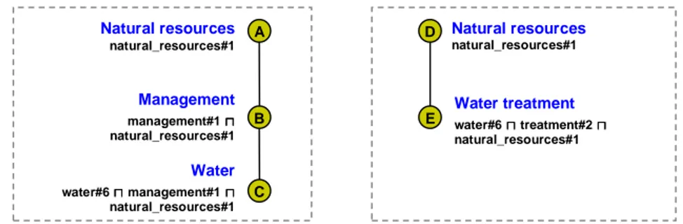
arcs between nodes represent subset relations. For instance, the extension of the con-cept “animal” is the set of documents about real world animals. Note that this is the semantics implicitly used in libraries. Many types of commonly used ontologies (such as on-line catalogs, file systems, web directories and library classifications) can be translated into lightweight ontologies. For instance, [12] describes how this can be done for LCSH and NALT. Each node label is translated into a logic formula repre-senting the meaning of the node taking into account its context, i.e. the path from the root to the node. Each atomic concept appearing in the formulas is taken from a con-trolled vocabulary, such as WordNet. A formal definition of lightweight ontology can be found in [4], while further information about the translation procedure can be found in [2]. Fig. 1 shows an example taken from [12]. It shows two classifications that are translated into lightweight ontologies following the procedure described in [2]. Natural language labels are shown in bold. Each formula is reported under the corresponding label. Each atomic concept (e.g. water#6) is represented by a string fol-lowed by a number representing the sense taken from a WordNet synset.
Fig. 1. Two lightweight ontologies 3.2 Minimal and redundant mappings
MinSMatch computes a set of semantic correspondences, called mapping elements, between two lightweight ontologies. A mapping element is defined as follows:
Definition 1 (Mapping element). Given two lightweight ontologies O1 and O2, a
mapping element m between them is a triple <n1, n2, R>, where:
a) n1∈N1 is a node in O1, called the source node;
b) n2∈N2 is a node in O2, called the target node;
c) R ∈ {⊥, ≡, ⊑, ⊒} is the strongest semantic relation holding between n1 and n2.
The strength of a semantic relation is established according to the partial order where disjointness precedes equivalence and more and less specific are unordered and follow equivalence. Under this ordering, MinSMatch always computes the strongest semantic relation holding between two nodes. In particular, it computes the minimal
mapping, i.e. the minimal subset of mapping elements between the two ontologies
such that all the others can be efficiently computed from them, and are therefore said to be redundant. The fundamental idea is that a mapping element m’ is redundant
Natural resources natural_resources#1 Natural resources natural_resources#1 Water treatment water#6 ⊓ ⊓ ⊓ ⊓ treatment#2 ⊓⊓⊓⊓ natural_resources#1 Management management#1 ⊓⊓⊓⊓ natural_resources#1 Water water#6 ⊓ ⊓ ⊓ ⊓ management#1 ⊓ ⊓ ⊓ ⊓ natural_resources#1 A B C D E
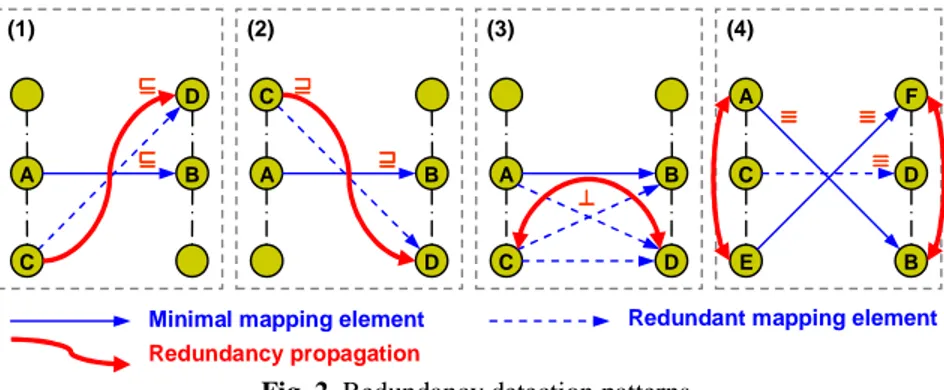
w.r.t. another mapping element m if the existence of m’ can be asserted simply by looking at the positions of its nodes w.r.t. the nodes of m in their respective ontolo-gies. The four redundancy patterns in Fig. 2, one for each semantic relation, cover all possible cases. A proof is given in [4]. The blue dashed elements are redundant w.r.t. the solid blue ones. The red solid curves show how a semantic relation propagates.
For instance, in pattern (1), the element <C, D, ⊑> is redundant w.r.t. <A, B, ⊑>. In fact, the chain of subsumptions C ⊑ A ⊑ B ⊑ D holds4 and therefore by transitivity we
can conclude that C ⊑ D. Notice that this still holds in case we substitute A ⊑ B with A ≡ B. Taking any two paths in the two ontologies, a minimal subsumption mapping element is an element with the highest node in one path whose formula is subsumed by the formula of the lowest node in the other path.
Fig. 2. Redundancy detection patterns
This can be codified in the following redundancy condition:
Definition 2 (Redundant mapping element). Given two lightweight ontologies O1
and O2, a mapping M and a mapping element m’∈M with m’ = <C, D, R’> between
them, we say that m’ is redundant in M iff one of the following holds:
(1) If R’ is ⊑, ∃m∈M with m = <A, B, R> and m ≠ m’ such that R ∈ {⊑, ≡≡≡≡}, A
∈ path(C) and D ∈ path(B);
(2) If R’ is ⊒, ∃m∈M with m = <A, B, R> and m ≠ m’ such that R ∈ {⊒, ≡}, C
∈ path(A) and B ∈ path(D);
(3) If R’ is ⊥, ∃m∈M with m = <A, B, ⊥> and m ≠ m’ such that A ∈ path(C) and B ∈ path(D);
(4) If R’ is ≡, conditions (1) and (2) must be satisfied.
Here path(n) is the path from the root to the node n. Note that we enforce m ≠ m’ to exclude the trivial situation in which a mapping element is compared with itself. We prove in [4] that it captures all and only the cases of logical redundancy (of a mapping element w.r.t. another one). This definition allows abstracting from logical inference to computing the redundant elements just by looking at the positions of the nodes in
4 This is because nodes in lightweight ontologies are connected through subsumption relations.
A B C D (1) ⊑ ⊑⊑ ⊑ ⊑ ⊑⊑ ⊑ A B (2) C D ⊒ ⊒ ⊒ ⊒ ⊒ ⊒⊒ ⊒ A B C (3) D C D E F (4) A B ≡ ≡ ≡ ≡ ≡ ≡ ≡ ≡ ⊥ ⊥ ⊥ ⊥ ≡ ≡≡ ≡
Minimal mapping element Redundancy propagation
the two trees. The notion of redundancy given above is fundamental to minimize the amount of calls to the logical reasoners and to reduce the problem of lack of back-ground knowledge. Given a mapping element m = <A, B, ⊒>, by looking for instance at pattern (2) in Fig. 2, we can observe that it is not necessary to compute the semantic relation holding between A and any descendant C in the sub-tree of B since we know in advance that it is ⊒. The minimal mapping is then defined as follows:
Definition 3 (Minimal mapping). Given two lightweight ontologies O1 and O2, we
say that a mapping M between them is minimal iff:
a) ∄m∈M such that m is redundant (minimality condition); b) ∄M’⊃M satisfying condition a) above (maximality condition).
A mapping element is minimal if it belongs to the minimal mapping.
Note that the conditions (a) and (b) ensure that the minimal set is the set of maxi-mum size with no redundant elements. We also prove that for any two given light-weight ontologies, the minimal mapping always exists and it is unique [4].
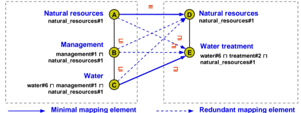
Minimal mappings provide clear usability advantages. Consider the example in Fig. 3 taken from [12]. It provides the minimal mapping (the solid arrows) and the maximum number of mapping elements, that we call the mapping of maximum size, between the two lightweight ontologies given in Fig. 1. Note that only the two solid ones are minimal, because all the others (the dashed ones) can be entailed from them. For instance, A ⊒ E follows from A ⊒ D for pattern (2). As we will show, the valida-tion phase can be faster if we concentrate on the minimal mapping. The key intuivalida-tion is that, if the user accepts as correct an element which is in the minimal set then all the inferred ones will be automatically validated as correct.
Fig. 3. The minimal and redundant mapping between two lightweight ontologies
4
The MinSMatch algorithm
At the top level the algorithm is organized as follows:
• Step 1, computing the minimal mapping modulo equivalence: compute the
set of disjointness and subsumption mapping elements which are minimal
⊑ ⊑ ⊑ ⊑ ⊒⊒⊒⊒ ≡ ≡ ≡ ≡ Natural resources natural_resources#1 Natural resources natural_resources#1 Water treatment water#6 ⊓ ⊓ ⊓ ⊓ treatment#2 ⊓⊓⊓⊓ natural_resources#1 Management management#1 ⊓⊓⊓⊓ natural_resources#1 Water water#6 ⊓ ⊓ ⊓ ⊓ management#1 ⊓ ⊓ ⊓ ⊓ natural_resources#1 ⊑ ⊑⊑ ⊑ ⊒⊒⊒⊒ ⊒ ⊒⊒ ⊒ A B C D E
modulo equivalence. By this we mean that they are minimal modulo
collaps-ing, whenever possible, two subsumption relations of opposite direction into a single equivalence mapping element;
• Step 2, computing the minimal mapping: collapse all the pairs of
subsump-tion elements (of opposite direcsubsump-tion) between the same two nodes into a single equivalence element. This will result in the minimal mapping;
• Step 3, computing the mapping of maximum size: Compute the mapping of
maximum size (including minimal and redundant mapping elements). During this step the existence of a (redundant) element is computed as the result of the propagation of the elements in the minimal mapping.
The first two steps are performed at matching time, while the third is activated on user request. The following three subsections analyze the three steps above in detail.
4.1 Step 1: Computing the minimal mapping modulo equivalence
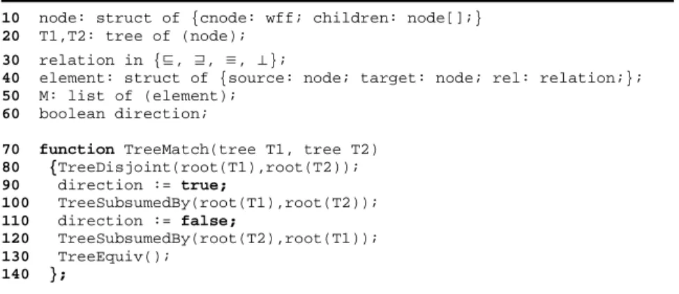
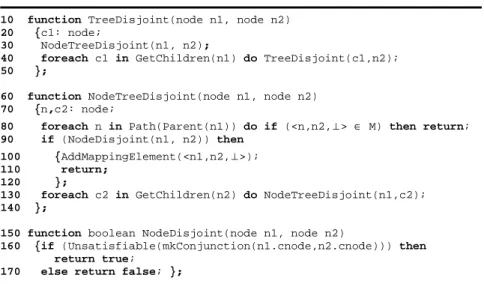
The minimal mapping is computed by a function TreeMatch whose pseudo-code is described in Fig. 4. M is the minimal set while T1 and T2 are the input lightweight ontologies. TreeMatch is called on the root nodes of T1 and T2. It is crucially de-pendent on the node matching functions NodeDisjoint (Fig. 5) and
NodeSubsum-edBy (Fig. 6) which take two nodes n1 and n2 and return a positive answer in case of
disjointness or subsumption, or a negative answer if it is not the case or they are not able to establish it. Notice that these two functions hide the heaviest computational costs; in particular their computation time is exponential when the relation holds and, exponential in the worst case, but possibly much faster, when the relation does not hold. The main motivation for this is that the node matching problem should be trans-lated into disjointness or subsumption problem in propositional DL.
10 node: struct of {cnode: wff; children: node[];} 20 T1,T2: tree of (node);
30 relation in {⊑, ⊒, ≡, ⊥};
40 element: struct of {source: node; target: node; rel: relation;}; 50 M: list of (element);
60 boolean direction;
70 function TreeMatch(tree T1, tree T2) 80 {TreeDisjoint(root(T1),root(T2)); 90 direction := true; 100 TreeSubsumedBy(root(T1),root(T2)); 110 direction := false; 120 TreeSubsumedBy(root(T2),root(T1)); 130 TreeEquiv(); 140 };
Fig. 4. Pseudo-code for the tree matching function
The goal, therefore, is to compute the minimal mapping by minimizing the calls to the node matching functions and, in particular minimizing the calls where the relation will turn out to hold. We achieve this purpose by processing both trees top down. To maximize the performance of the system, TreeMatch has therefore been built as the
sequence of three function calls: the first call to TreeDisjoint (line 80) computes the minimal set of disjointness mapping elements, while the second and the third call to
TreeSubsumedBy compute the minimal set of subsumption mapping elements in the
two directions modulo equivalence (lines 90-120). Notice that in the second call,
TreeSubsumedBy is called with the input ontologies with swapped roles. These three
calls correspond to Step 1 above. Line 130 in the pseudo code of TreeMatch imple-ments Step 2 and it will be described in the next subsection.
TreeDisjoint (Fig. 5) is a recursive function which finds all disjointness minimal
elements between the two sub-trees rooted in n1 and n2. Following the definition of redundancy, it basically searches for the first disjointness element along any pair of paths in the two input trees. Exploiting the nested recursion of NodeTreeDisjoint in-side TreeDisjoint, for any node n1 in T1 (traversed top down, depth first)
Node-TreeDisjoint visits all of T2, again top down, depth first. NodeNode-TreeDisjoint (called
at line 30, starting at line 60) keeps fixed the source node n1 and iterates on the whole target sub-tree below n2 till, for each path, the highest disjointness element, if any, is found. Any such disjoint element is added only if minimal (lines 90-120). The condi-tion at line 80 is necessary and sufficient for redundancy. The idea here is to exploit the fact that any two nodes below two nodes involved in a disjointness mapping ele-ment are part of a redundant eleele-ment and, therefore, to stop the recursion thus saving a lot of time expensive calls (n*m calls with n and m the number of the nodes in the two trees). Notice that this check needs to be performed on the full path.
NodeDis-joint checks whether the formula obtained by the conjunction of the formulas
associ-ated to the nodes n1 and n2 is unsatisfiable (lines 150-170).
10 function TreeDisjoint(node n1, node n2) 20 {c1: node;
30 NodeTreeDisjoint(n1, n2);
40 foreach c1 in GetChildren(n1) do TreeDisjoint(c1,n2); 50 };
60 function NodeTreeDisjoint(node n1, node n2) 70 {n,c2: node;
80 foreach n in Path(Parent(n1)) do if (<n,n2,⊥> ∈ M) then return;
90 if (NodeDisjoint(n1, n2)) then 100 {AddMappingElement(<n1,n2,⊥>);
110 return; 120 };
130 foreach c2 in GetChildren(n2) do NodeTreeDisjoint(n1,c2); 140 };
150 function boolean NodeDisjoint(node n1, node n2)
160 {if (Unsatisfiable(mkConjunction(n1.cnode,n2.cnode))) then return true;
170 else return false; };
Fig. 5. Pseudo-code for the TreeDisjoint function
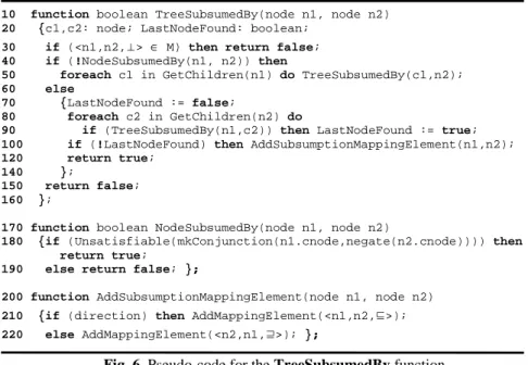
TreeSubsumedBy (Fig. 6) recursively finds all minimal mapping elements where
the strongest relation between the nodes is ⊑ (or dually, ⊒ in the second call; in the following we will concentrate only on the first call).
10 function boolean TreeSubsumedBy(node n1, node n2) 20 {c1,c2: node; LastNodeFound: boolean;
30 if (<n1,n2,⊥> ∈ M) then return false;
40 if (!NodeSubsumedBy(n1, n2)) then
50 foreach c1 in GetChildren(n1) do TreeSubsumedBy(c1,n2); 60 else
70 {LastNodeFound := false;
80 foreach c2 in GetChildren(n2) do
90 if (TreeSubsumedBy(n1,c2)) then LastNodeFound := true; 100 if (!LastNodeFound) then AddSubsumptionMappingElement(n1,n2); 120 return true;
140 };
150 return false; 160 };
170 function boolean NodeSubsumedBy(node n1, node n2)
180 {if (Unsatisfiable(mkConjunction(n1.cnode,negate(n2.cnode)))) then return true;
190 else return false; };
200 function AddSubsumptionMappingElement(node n1, node n2) 210 {if (direction) then AddMappingElement(<n1,n2,⊑>);
220 else AddMappingElement(<n2,n1,⊒>); };
Fig. 6. Pseudo-code for the TreeSubsumedBy function
Notice that TreeSubsumedBy assumes that the minimal disjointness elements are already computed; thus, at line 30 it checks whether the mapping element between the nodes n1 and n2 is already in the minimal set. If this is the case it stops the recursion. This allows computing the stronger disjointness relation rather than subsumption when both hold (namely with an inconsistent node). Given n2, lines 40-50 implement a depth first recursion in the first tree till a subsumption is found. The test for sub-sumption is performed by NodeSubsumedBy that checks whether the formula ob-tained by the conjunction of the formulas associated to the node n1 and the negation of the formula for n2 is unsatisfiable (lines 170-190). Lines 60-140 implement what happens after the first subsumption is found. The key idea is that, after finding the first subsumption, TreeSubsumedBy keeps recursing down the second tree till it finds the last subsumption. When this happens, the resulting mapping element is added to the minimal mapping (line 100). Notice that both NodeDisjoint and
Node-SubsumedBy call the function Unsatisfiable which embeds a call to a SAT solver.
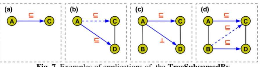
To fully understand TreeSubsumedBy, the reader should check what happens in the four situations in Fig. 7. In case (a) the first iteration of the TreeSubsumedBy finds a subsumption between A and C. Since C has no children, it skips lines 80-90 and directly adds the mapping element <A, C, ⊑> to the minimal set (line 100). In case (b), since there is a child D of C the algorithm iterates on the pair A-D (lines 80-90) finding a subsumption between them. Since there are no other nodes under D, it adds the mapping element <A, D, ⊑> to the minimal set and returns true. Therefore LastNodeFound is set to true (line 90) and the mapping element between the pair A-C is recognized as redundant. Case (c) is similar. The difference is that
com-putation of minimal disjointness mapping elements, and therefore the mapping ele-ment <A, C, ⊑> is recognized as minimal. In case (d) the algorithm iterates after the second subsumption mapping element is identified. It first checks the pair A-C and it-erates on A-D concluding that subsumption does not hold between them (line 40). Therefore, it recursively calls TreeSubsumedBy between B and D. In fact, since <A, C, ⊑> will be recognized as minimal, it is not worth checking <B, C, ⊑> for pattern (1). As a consequence <B, D, ⊑> is recognized as minimal together with <A, C, ⊑>.
Fig. 7. Examples of applications of the TreeSubsumedBy
Five observations. The first is that, even if, overall, TreeMatch implements three loops instead of one, the wasted (linear) time is largely counterbalanced by the expo-nential time saved by avoiding a lot of useless calls to the SAT solver. The second is that, when the input trees T1 and T2 are two nodes, TreeMatch behaves as a node matching function which returns the semantic relation holding between the input nodes. The third is that the call to TreeDisjoint before the two calls to
TreeSubsum-edBy allows us to implement the partial order on relations defined in the previous
section. In particular it allows returning only a disjointness mapping element when both disjointness and subsumption hold (see Definition 2 of mapping). The fourth is that, in the body of TreeDisjoint, the fact that the two sub-trees where disjointness holds are skipped is what allows not only implementing the partial order (see the pre-vious observation) but also saving a lot of useless calls to the node matching functions (line 2). The fifth and last observation is that the implementation of TreeMatch cru-cially depends on the fact that the minimal elements of the two directions of subsump-tion and disjointness can be computed independently (modulo inconsistencies).
4.2 Step 2: Computing the minimal mapping
The output of Step 1 is the set of all disjointness and subsumption mapping elements which are minimal modulo equivalence. The final step towards computing the mini-mal mapping is that of collapsing any two subsumption relations, in the two direc-tions, holding between the same two nodes into a single equivalence relation. The tricky part here is that equivalence is in the minimal set only if both subsumptions are in the minimal set. We have three possible situations:
1. None of the two subsumptions is minimal (in the sense that it has not been computed as minimal in Step 1): nothing changes and neither subsumption nor equivalence is memorized as minimal;
2. Only one of the two subsumptions is minimal while the other is not minimal (again according to Step 1): this case is solved by keeping only the subsump-tion mapping as minimal. Of course, during Step 3 (see below) the necessary
C A ⊑ ⊑ ⊑ ⊑ D C A ⊑ ⊑ ⊑ ⊑ (a) (b) ⊑ ⊑ ⊑ ⊑ B D C A ⊑ ⊑⊑ ⊑ (c) ⊥ ⊥⊥ ⊥ B D C A ⊑ ⊑⊑ ⊑ (d) ⊑ ⊑ ⊑ ⊑ ⊑ ⊑ ⊑ ⊑
computations will have to be done in order to show to the user the existence of an equivalence relation between the two nodes;
3. Both subsumptions are minimal (from Step 1): in this case the two subsump-tions can be deleted and substituted with a single equivalence element. Notice that Step 3 can be computed very easily in time linear with the number of mapping elements output of Step 1: it is sufficient to check for all the subsumption elements of opposite direction between the same two nodes and to substitute them with an equivalence element. This is performed by function TreeEquiv in Fig. 4.
4.3 Step 3: Computing the mapping of maximum size
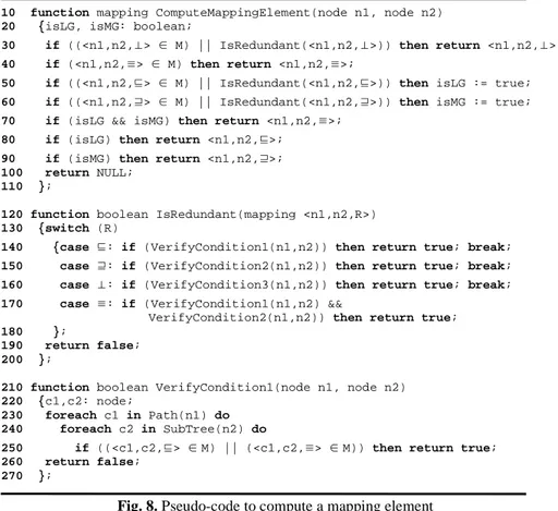
For brevity we concentrate on the following problem: given two lightweight ontolo-gies T1 and T2 and the of minimal mapping M compute the mapping element be-tween two nodes n1 in T1 and n2 in T2 or the fact that no element can be computed given the current available background knowledge. Pseudo-code is given in Fig. 8.
10 function mapping ComputeMappingElement(node n1, node n2) 20 {isLG, isMG: boolean;
30 if ((<n1,n2,⊥> ∈ M) || IsRedundant(<n1,n2,⊥>)) then return <n1,n2,⊥>;
40 if (<n1,n2,≡> ∈ M) then return <n1,n2,≡>;
50 if ((<n1,n2,⊑> ∈ M) || IsRedundant(<n1,n2,⊑>)) then isLG := true;
60 if ((<n1,n2,⊒> ∈ M) || IsRedundant(<n1,n2,⊒>)) then isMG := true;
70 if (isLG && isMG) then return <n1,n2,≡>;
80 if (isLG) then return <n1,n2,⊑>;
90 if (isMG) then return <n1,n2,⊒>;
100 return NULL; 110 };
120 function boolean IsRedundant(mapping <n1,n2,R>) 130 {switch (R)
140 {case ⊑: if (VerifyCondition1(n1,n2)) then return true; break;
150 case ⊒: if (VerifyCondition2(n1,n2)) then return true; break;
160 case ⊥: if (VerifyCondition3(n1,n2)) then return true; break;
170 case ≡: if (VerifyCondition1(n1,n2) &&
VerifyCondition2(n1,n2)) then return true;
180 };
190 return false; 200 };
210 function boolean VerifyCondition1(node n1, node n2) 220 {c1,c2: node;
230 foreach c1 in Path(n1) do 240 foreach c2 in SubTree(n2) do
250 if ((<c1,c2,⊑> ∈ M) || (<c1,c2,≡> ∈ M)) then return true;
260 return false; 270 };
ComputeMappingElement is structurally very similar to the NodeMatch function
described in [27], modulo the key difference that no calls to SAT are needed.
Com-puteMappingElement always returns the strongest mapping element. The test for
re-dundancy performed by IsRedundant reflects the definition of rere-dundancy provided in Section 3 above. For lack of space, we provide below only the code which does the check for the first pattern; the others are analogous. Given for example a mapping element <n1, n2, ⊑>, condition 1 is verified by checking whether in M there is an element <c1, c2, ⊑> or <c1, c2, ≡> with c1 ancestor of n1 and c2 descendant of n2. Notice that ComputeMappingElement calls IsRedundant at most three times and, therefore, its computation time is linear with the number of mapping elements in M.
5
Mapping validation
Validating means taking a decision about the correctness of the correspondences sug-gested by the system [6]. We say that the user positively validates a correspondence, or simply accepts it, if he accepts it as correct, while we say that the user negatively
validates a correspondence, or simply rejects it, if he does not accept it as correct.
Both rejected and accepted correspondences have to be marked to record the decision. We use MinSMatch to compute the initial minimal mapping. Focusing on the ele-ments in this set minimizes the work load of the user. In fact, they represent the mini-mum amount of information which has to be validated as it consequently results in the validation of the rest of the (redundant) elements.
5.1 Validation sequence
The system has to suggest step by step the order of correspondences to be validated. In particular, this order must follow the partial order over the mapping elements de-fined in [4]. As also described in [12], the intuition is that if an element m is judged as correct during validation, all mapping elements derived by m are consequently cor-rect. Conversely, if m is judged as incorrect we need to include in the minimal set the maximal elements from the set of mapping elements derived by m, that we call the
sub-minimal elements of m, and ask the user to validate them.
For instance, for the mapping in Fig. 3, in the case <A, D, ≡> is rejected, we need to validate the maximal elements in the set {<A, E, ⊒>, <B, D, ⊑>, <C, D, ⊑>} of elements derived by m. They are <A, E, ⊒> and <B, D, ⊑>. The element <C, D, ⊑> needs to be validated only in the case when <B, D, ⊑> is further rejected. Sub-minimal elements can be efficiently computed (see next section).
Note that, for a better understanding of the correspondences, it is important to show to the user the strongest semantic relation holding between the nodes, even if it is not in the minimal set. For example, showing equivalence where only a direction of the subsumption is minimal.
5.2 User interaction during validation
The validation process is illustrated in Fig. 9. The minimal mapping M between the two lightweight ontologies T1 and T2 is computed by the TreeMatch (line 10)
de-scribed in the previous section and validated by the function Validate (line 20). At the end of the process, M will contain only the mapping elements accepted by the user. The Validate function is given at lines 30-90. The validation process is carried out in a top-down fashion (lines 40-50). This is to evaluate in sequence the elements that share as much contextual information as possible. This in turn reduces the cognitive load requested to the user to take individual decisions. The presence of an element m between two nodes n1 and n2 in M is tested by the function GetElement (line 60). In positive case the function returns it, otherwise NULL is returned. Each element is then validated using the function ValidateElement (line 70), whose pseudo-code is given in Fig. 10. The process ends when all the nodes in the two trees have been proc-essed. A possible optimization consists in stopping the process when all the elements in M have been processed.
10 M := TreeMatch(T1, T2); 20 Validate(M);
30 function void Validate(list of (element) M) 40 { foreach n1 in T1 do 50 foreach n2 in T2 do { 60 m := GetElement(M, n1, n2); 70 if (m != NULL) ValidateElement(m); 80 } 90 };
Fig. 9. The validation process of the minimal mapping M
10 function void ValidateElement(element m) 20 { S: list of (element);
30 if IsValid(m) AddElement(m, M); 40 else {
50 RemoveElement(m, M); 60 S := GetSubminimals(m);
70 foreach m in S do { if (!IsRedundant(m)) ValidateElement(m); } 80 }
90 };
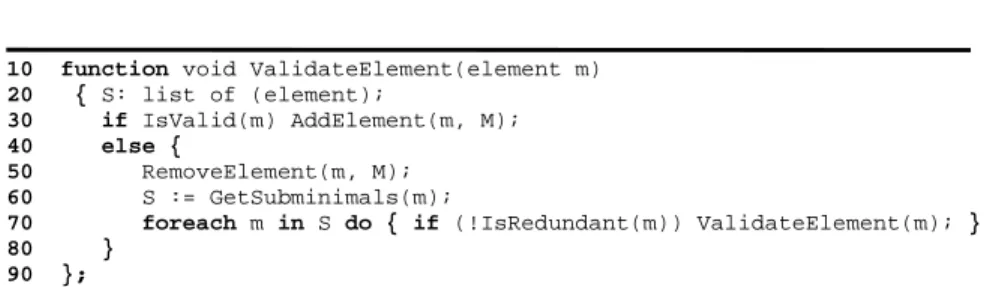
Fig. 10. The validation process of a single element m
The validation of a single element m is embedded in the ValidateElement func-tion. The correctness of m is established through a call to the function IsValid (line 30), that takes care of the communication with the user. The user can accept or reject
m. If m is accepted, m is added to the set M using the function AddElement (line 30).
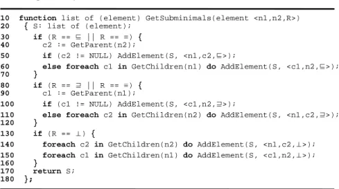
Note that this is necessary when the ValidateElement is called on a sub-minimal element at line 70. Otherwise, if m is rejected, it is removed from M using the tion RemoveElement (line 50) and its sub-minimal elements, computed by the func-tion GetSubminimals (line 60), are recursively validated (line 70). The pseudo-code for the GetSubminimals function is in Fig. 11. It applies the rules for propagation suggested in [4] to identify the elements that follow an element m in the partial order.
Two observations are needed. The first is that a sub-minimal element can be re-dundant w.r.t. more than one element in M. In these cases we postpone their valida-tion to the validavalida-tion of the elements for which they are redundant. For instance, <A,
E, ⊒> is redundant w.r.t. both <A, D, ≡> and <C, E, ⊒> in Fig. 3. Therefore, the vali-dation of <A, E, ⊒> is postponed to the validation of <C, E, ⊒>. In other words, if <C, E, ⊒> is positively validated, then it will be superfluous asking the user to validate <A, E, ⊒>. We use the function IsRedundant described in [4] (line 70) for this. This also avoids validating the same element more than once. The second is that, in order to keep the strongest relation between two nodes, the following rules are enforced:
(a) if we add to M two subsumptions of opposite directions for the same pair of nodes, we collapse them into equivalence;
(b) if we add an equivalence between two nodes, it substitutes any subsumption previously inserted between the same nodes, but it is ignored if we already have in M a disjointness between these nodes;
(c) if we add a disjointness between two nodes, it substitutes any other relation previously inserted in M between the same nodes.
10 function list of (element) GetSubminimals(element <n1,n2,R>) 20 { S: list of (element);
30 if (R == ⊑ || R == ≡) {
40 c2 := GetParent(n2);
50 if (c2 != NULL) AddElement(S, <n1,c2,⊑>);
60 else foreach c1 in GetChildren(n1) do AddElement(S, <c1,n2,⊑>);
70 }
80 if (R == ⊒ || R == ≡) {
90 c1 := GetParent(n1);
100 if (c1 != NULL) AddElement(S, <c1,n2,⊒>);
110 else foreach c2 in GetChildren(n2) do AddElement(S, <n1,c2,⊒>);
120 }
130 if (R == ⊥) {
140 foreach c2 in GetChildren(n2) do AddElement(S, <n1,c2,⊥>);
150 foreach c1 in GetChildren(n1) do AddElement(S, <c1,n2,⊥>);
160 }
170 return S; 180 };
Fig. 11. The function for the identification of the sub-minimal elements
6
Evaluation
We have tested MinSMatch on datasets commonly used to evaluate matching tools [21]. Their short description is in [4, 21]. Table 1 summarizes their characteristics.
# Dataset pair Node count Max depth Average
branching factor
1 Cornell/Washington 34/39 3/3 5.50/4.75
2 Topia/Icon 542/999 2/9 8.19/3.66
3 Source/Target 2857/6628 11/15 2.04/1.94
4 Eclass/Unspsc 3358/5293 4/4 3.18/9.09
Table 1. Complexity of the datasets
Table 2 shows the percentage of reduction in the number of elements contained in the minimal mapping w.r.t. the mapping of maximum size. The reduction is
calcu-lated as (1-m/t), where m is the number of elements in the minimal set and t is the to-tal number of elements in the mapping of maximum size. We have a significant re-duction, in the range 68-96%.
MinSMatch # Mapping of maximum size, elements (t) Minimal mapping, elements (m) Reduction, % 1 223 36 83.86 2 5491 243 95.57 3 282648 30956 89.05 4 39818 12754 67.97
Table 2. Mapping sizes and percentage of reduction on standard datasets
As described in [12], we have also conducted experiments with NALT and LCSH. As reported in Table 3, these experiments show that the reduction in the number of correspondences can reach 99%. In other words, this means that by concentrating on minimal mappings we can save up to 99% of the manual checks required for mapping validation.
Id Source Branch
A NALT Chemistry and Physics
B NALT Natural Resources, Earth and Environmental Sciences
C LCSH Chemical Elements
D LCSH Chemicals
E LCSH Management
F LCSH Natural resources
Branches Mapping of maximum
size, elements (t) Minimal mapping, elements (m) Reduction, % A vs. C 17716 7541 57,43 A vs. D 139121 994 99,29 A vs. E 9579 1254 86,91 B vs. F 27191 1232 95,47
Table 3. Mapping sizes and percentage of reduction on NALT and LCSH
Finally, we have compared MinSMatch w.r.t. the state of the art matcher S-Match [22]. Table 4 shows the reduction in computation time and calls to the logical reason-ers. As it can be noticed, the reductions are substantial.
Run Time, ms Calls to logical reasoners (SAT)
# S-Match MinSMatch Reduction,
%
S-Match MinSMatch Reduction,
%
1 472 397 15.88 3978 2273 42.86
2 141040 67125 52.40 1624374 616371 62.05
3 3593058 1847252 48.58 56808588 19246095 66.12
4 6440952 2642064 58.98 53321682 17961866 66.31
Table 4. Run time and SAT problems
7
Conclusions and future work
We have discussed limitations of existing matching tools. We have observed that, once the initial mapping has been computed by the system, current tools provide poor support (or no support at all) for its validation and maintenance in time. In addition,
current visualization tools are cognitively demanding, hardly scale with the increasing number of nodes and the resulting visualizations are rather messy. We have proposed the use of MinSMatch for the computation of the minimal mapping and showed that, by concentrating on the correspondences in the minimal set, the amount of manual checks necessary for validation can be reduced up to two orders of magnitude. We have also showed that by minimizing the number of calls to logical reasoners, the MinSMatch algorithm is significantly faster w.r.t. state of the art semantic matching tools and reduces the problem of lack of background knowledge.
Yet, maintaining a mapping in time is an extremely complex and still largely unex-plored task. Even a trivial change of a node label can have an enormous impact on the correspondences starting or terminating in this node and all the nodes in their respec-tive subtrees. In future we plan to further explore these problems and develop a user interface which follows the specifications provided in this paper.
Acknowledgments. The research leading to these results has received funding from
the European Community's Seventh Framework Programme (FP7/2007-2013) under grant agreement n° 231126 LivingKnowledge: LivingKnowledge – Facts, Opinions and Bias in Time
References
1. P. Shvaiko, J. Euzenat, 2007. Ontology Matching. Springer-Verlag New York, Inc. Secau-cus, NJ, USA.
2. F. Giunchiglia, M. Marchese, I. Zaihrayeu, 2006. Encoding Classifications into Light-weight Ontologies. Journal of Data Semantics 8, pp. 57-81.
3. F. Giunchiglia, P. Shvaiko, M. Yatskevich, 2006. Discovering missing background knowl-edge in ontology matching. In Proc. of ECAI 2006, pp. 382–386.
4. F. Giunchiglia, V. Maltese, A. Autayeu, 2008. Computing minimal mappings. At the 4th Ontology Matching Workshop at the ISWC 2009.
5. G. G. Robertson, M. P. Czerwinski, J. E. Churchill, 2005. Visualization of mappings be-tween schemas. Proc. of SIGCHI Conference on Human Factors in Computing Systems. 6. S. Falconer, M. Storey, 2007. A cognitive support framework for ontology mapping. In
Proc. of ISWC/ASWC, 2007.
7. A. Halevy, 2005. Why your data won’t mix. ACM Queue, 3(8): pp. 50–58.
8. A. Katifory, C. Halatsis, G. Lepouras, C. Vassilakis, E. Giannopoulou, 2007. Ontology vi-sualization methods - a survey. ACM Comput. Surv. 39, 4, 10.
9. S. R. Ranganathan, 1965. The Colon Classification. In S. Artandi, editor, Vol IV of the Rutgers Series on Systems for the Intellectual Organization of Information. New Bruns-wick, NJ: Graduate School of Library Science, Rutgers University.
10. F. Giunchiglia and I. Zaihrayeu, 2008. Lightweight ontologies. In S. LNCS, editor, Ency-clopedia of Database Systems, 2008.
11. F. Giunchiglia, B. Dutta, V. Maltese, 2009. Faceted lightweight ontologies. In “Concep-tual Modeling: Foundations and Applications”, A. Borgida, V. Chaudhri, P. Giorgini, Eric Yu (Eds.) LNCS 5600 Springer (2009).
12. F. Giunchiglia, D. Soergel, V. Maltese, A. Bertacco, 2009. Mapping large-scale Knowl-edge Organization Systems.
13. P. Shvaiko, J. Euzenat, 2008. Ten Challenges for Ontology Matching. In Proc. of the 7th Int. Conference on Ontologies, Databases, and Applications of Semantics (ODBASE). 14. P. Shvaiko, F. Giunchiglia, P. P. da Silva, D. L. McGuinness, 2005. Web Explanations for
15. T. Koch, H. Neuroth, M. Day, 2003. Renardus: Cross-browsing European subject gate-ways via a common classification system (DDC). In I.C. McIlwaine (Ed.), Subject re-trieval in a networked environment. Proc. of the IFLA satellite meeting, pp. 25–33. 16. D. Vizine-Goetz, C. Hickey, A. Houghton, R. Thompson, 2004. Vocabulary Mapping for
Terminology Services”. Journal of Digital Information 4(4)(2004), Article No. 272. 17. C. Whitehead, 1990. Mapping LCSH into Thesauri: the AAT Model. In Beyond the Book:
Extending MARC for Subject Access, pp. 81.
18. E. O'Neill, L. Chan, 2003. FAST (Faceted Application for Subject Technology): A Simpli-fied LCSH-based Vocabulary. World Library and Information Congress: 69th IFLA Gen-eral Conference and Council, 1-9 August, Berlin.
19. D. Nicholson, A. Dawson, A. Shiri, 2006. HILT: A pilot terminology mapping service with a DDC spine. Cataloging & Classification Quarterly, 42 (3/4). pp. 187-200. 20. B. Lauser, G. Johannsen, C. Caracciolo, J. Keizer, W. R. van Hage, P. Mayr, 2008.
Com-paring human and automatic thesaurus mapping approaches in the agricultural domain. Proc. Int’l Conf. on Dublin Core and Metadata Applications.
21. P. Avesani, F. Giunchiglia and M. Yatskevich, 2005. A Large Scale Taxonomy Mapping Evaluation. In Proc. of International Semantic Web Conference (ISWC 2005), pp. 67-81. 22. F. Giunchiglia, M. Yatskevich, P. Shvaiko, 2007. Semantic Matching: algorithms and
im-plementation. Journal on Data Semantics, IX, 2007.
23. H. Stuckenschmidt, L. Serafini, H. Wache, 2006. Reasoning about Ontology Mappings. In Proc. of the ECAI-06 Workshop on Contextual Representation and Reasoning.
24. C. Meilicke, H. Stuckenschmidt, A. Tamilin, 2006. Improving automatically created map-pings using logical reasoning. In Proc. of the 1st International Workshop on Ontology Matching OM-2006, CEUR Workshop Proceedings Vol. 225.
25. C. Meilicke, H. Stuckenschmidt, A. Tamilin, 2008. Reasoning support for mapping revi-sion. Journal of Logic and Computation, 2008.
26. A. Borgida, L. Serafini. Distributed Description Logics: Assimilating Information from Peer Sources. Journal on Data Semantics pp. 153-184.
27. F. Giunchiglia, M. Yatskevich, P. Shvaiko, 2007. Semantic Matching: algorithms and im-plementation. Journal on Data Semantics, IX, 2007.