DISA W
OR
KING
P
APER
DISA
Dipartimento di Informatica
e Studi Aziendali
2008/5
Characteristic function estimation of
non-Gaussian Ornstein-Uhlenbeck
processes
DISA
Dipartimento di Informatica
e Studi Aziendali
A bank covenants pricing model
Flavio Bazzana
DISA W
OR
KING
P
APER
2008/5
Characteristic function estimation of
non-Gaussian Ornstein-Uhlenbeck
processes
DISA Working Papers
The series of DISA Working Papers is published by the Department of Computer and Management Sciences (Dipartimento di Informatica e Studi Aziendali DISA) of the University of Trento, Italy.
Editor
Ricardo Alberto MARQUES PEREIRA [email protected]
Managing editor
Roberto GABRIELE [email protected]
Associate editors
Flavio BAZZANA fl [email protected] Finance
Michele BERTONI [email protected] Financial and management accounting Pier Franco CAMUSSONE [email protected] Management information systems Luigi COLAZZO [email protected] Computer Science
Michele FEDRIZZI [email protected] Mathematics Andrea FRANCESCONI [email protected] Public Management
Loris GAIO [email protected] Business Economics
Umberto MARTINI [email protected] Tourism management and marketing Pier Luigi NOVI INVERARDI [email protected] Statistics
Marco ZAMARIAN [email protected] Organization theory
Technical offi cer
Paolo FURLANI [email protected]
Guidelines for authors
Papers may be written in English or Italian but authors should provide title, abstract, and keywords in both languages. Manuscripts should be submitted (in pdf format) by the corresponding author to the appropriate Associate Editor, who will ask a member of DISA for a short written review within two weeks. The revised version of the manuscript, together with the author's response to the reviewer, should again be sent to the Associate Editor for his consideration. Finally the Associate Editor sends all the material (original and fi nal version, review and response, plus his own recommendation) to the Editor, who authorizes the publication and assigns it a serial number.
The Managing Editor and the Technical Offi cer ensure that all published papers are uploaded in the international RepEc public-action database. On the other hand, it is up to the corresponding author to make direct contact with the Departmental Secretary regarding the offprint order and the research fund which it should refer to.
Ricardo Alberto MARQUES PEREIRA
Dipartimento di Informatica e Studi Aziendali Università degli Studi di Trento
Characteristic function estimation of non-Gaussian
Ornstein-Uhlenbeck processes
Emanuele Taufer∗
Abstract
Continuous non-Gaussian stationary processes of the OU-type are becoming increasingly popu-lar given their flexibility in modelling stylized features of financial series such as asymmetry, heavy tails and jumps. The use of non-Gaussian marginal distributions makes likelihood analysis of these processes unfeasible for virtually all cases of interest. This paper exploits the self-decomposability of the marginal laws of OU processes to provide explicit expressions of the characteristic function which can be applied to several models as well as to develop efficient estimation techniques based on the empirical characteristic function. Extensions to OU-based stochastic volatility models are provided.
Keywords: Ornstein-Uhlenbeck process, L´evy process, self-decomposable distribution,
character-istic function, estimation.
MSC : 62F10, 62F12, 62M05.
1
Introduction
A continuous stationary process {X(t), t ≥ 0} is defined to be of the Ornstein-Uhlenbeck type (OU for short) if it is the solution of the stochastic differential equation
dX(t) = −λX(t)dt + d `Z(t); (1.1)
here λ > 0 and `Z(t) is a homogeneous L´evy process, commonly referred to as the background driving
L´evy process (BDLP), for which E[log(1 + | `Z(1)|)] < ∞. The modelling via the use of general L´evy
processes, other than Brownian motion, allows to introduce specific non-Gaussian distributions for the marginal law of X(t) and has received considerable attention in recent literature in an attempt to accomodate features such as jumps, semi-heavy tails and asymmetry which are well evident in real phenomena and are a point of remarkable interest in fields of application such as finance and econometrics.
Among recent contributions we find a completely new class of models, termed non-Gaussian Ornstein-Uhlenbeck models by which, stochastic processes with given correlation structure and (possibly non-Gaussian) marginal distribution are constructed; see Barndorff-Nielsen (1998, 2001), Barndorff-Nielsen et Al. (1998), Barndorff-Nielsen and Shephard (2001, 2003), Barndorff-Nielsen
∗Department of Computer and Management Sciences, University of Trento, Via Inama 5, 38100 Trento - Italy,
and Leonenko (2005). Most notable examples include OU processes with marginal distributions such as the Normal Inverse Gaussian and the Inverse Gaussian (Barndorff-Nielsen, 1998), the Variance Gamma (Seneta, 2004), the Meixner (Schoutens and Teugel, 1998), the Normal and the Gamma. OU processes with positive jumps (subordinators) with marginal distributions such as the Inverse Gaussian are as well used as building blocks of stochastic volatility models (Barndorff-Nielsen and Shephard, 2001).
One of the key concepts related with these processes is that of self-decomposability. Recall that a random variable X is self-decomposable if, for all c ∈ (0, 1), there exists a characteristic
function (ch.f.) φc(ζ) such that the ch.f. of X, φ(ζ), can be decomposed as φ(ζ) = φ(cζ)φc(ζ).
Self-decomposability is closely related to stationary linear autoregressive time series of order 1, i.e. an AR(1) process. Essentially the only possible AR(1) processes are those for which the one-dimensional marginal law is self-decomposable and similarly for the OU process, i.e. an ”AR(1)” in continuous time. The peculiar form of the ch.f. of X(t) and its relation with the ch.f. of the underlying L´evy process has been exploited in Taufer and Leonenko (2008) to provide fast and reliable simulation procedures for OU processes. In this paper it will form the basis for providing explicit estimation procedures. With some more detail, it will be assumed that the marginal law of X(t) belongs to a parametric family indexed by a parameter vector, and it will be discussed how to implement estimation of the parameters appearing in (1.1), including λ, by exploiting the empirical ch.f..
Efficient estimation of OU processes in the non-Gaussian case maybe quite cumbersome to im-plement. Usually one has availability of observations at discrete time points because continuous data are hardly available in practice or not economical to observe. Although in theory, a likelihood could be constructed by exploiting the markov property or independence of increments, one in practice has rarely availability of explicit or tractable expressions for the relevant densities. One way out is to resort to simulation based techniques, as it has been discussed in Barndorff-Nielsen (1998) or, in the context of OU stochastic volatility processes, by Roberts et al. (2004), Griffin and Steel (2006), Gander and Stephens (2007a, 2007b). The problem with these methods is that simulation of OU, and more generally, L´evy processes, is difficult owing to their jump character and one usually has to resort to approximations. Also, simulation based techniques are usually implemented more easily for subordinators rather than for general OU processes; for further details and references on simulation of L´evy processes see Todorov and Tauchen (2006). On the other hand, Jongbloed et al. (2005) and Jongbloed and Van der Meulen (2006) propose, respectively, non-parametric and parametric estimators of the L´evy density for subordinators; their estimators are based on the empirical cumu-lant function and in this sense they are close to those defined here. The approach of this paper is more general as it is not restricted to processe with positive jumps: by providing rules for easily constructing the estimators starting from the univariate ch.f. of X(t), which is available in explicit form for several models of interest, a unified approach to ch.f. estimation of OU processes is intro-duced; previous literature concentrates mostly on processes with positive jumps, while the general case may turn quite complicated. Exploiting the peculiarity of self-decomposable random variables will allow to completely circumvent problems encountered with other techniques. Other works of in-terest here are those of Neumanna and Reiss (2008) which consider non-parametric estimation of the L´evy characteristic of general L´evy processes, Woerner (2004) which considers estimation of skewness parameter for L´evy processes and, for the Gaussian case, Baran, Pap, and van Zuijlen (2003), Gloter (2001), Florens-Landais and Pham (1999), Pap and van Zuijlen (1996) and the references therein.
Estimation based on the empirical ch.f. is well established and a good starting point is the paper of Feuerverger and McDunnough (1981) which show that arbitrarily high levels of efficiency can be
obtained by such methods in the i.i.d. case; furthermore, they discuss the extension to dependent observations. Other references that are relevant to the subsequent development are those of Madan and Seneta (1987), Feuerverger (1990), Knight and Satchell (1997) and Knight and Yu (2002), Jiang and Knight (2002) which discuss in more depth empirical ch.f. estimation in a non i.i.d. setting. The contribution of this paper builds on previous literature in more ways: by implementing the procedure for a large variety of OU processes; by presenting a method that requires neither discretization nor simulation; by providing exact expressions for moments and ch.f. of OU processes; by comparing two approaches: one based on the bivariate ch.f of (1.1), the other based on the ch.f. of the ’error’ term of the discretely observed process; this last approach may be seen as an attempt to substitue likelihood analisys of (1.1) based on i.i.d. observations.
This paper is organized as follows. The next section will provide some background information and some results on ch.f. of OU processes needed for estimation purposes. In section 3 the estimators are defined and their asymptotic properties studied. Section 4 is devoted to applications with simu-lated and real data. Section 5 discusses an extension of the ch.f. technique to OU based stochastic volatility models. The appendix provides the proofs of the results presented in the previous sections.
2
Characteristic functions and OU processes
The present section reviews some known results; for further details and generalizations the reader is referred to Wolfe (1982), Barndorff-Nielsen et Al. (1998), Barndorff-Nielsen (2001), Sato (1999). Equation (1.1) has a strong solution of the form
X(t) = e−λtX(0) + ε(λ)(t). (2.2)
where ε(λ)(t) is an error term, independent of X(0), which is given by
ε(λ)(t) =
Z t
0
e−λ(t−s)d `Z(s). (2.3)
Define the ch.f. of X(t) and ε(λ)(t) as
φ(ζ) = E(eiζX(t)), ϕt(ζ) = E(eiζε
(λ)(t)
). (2.4)
Also, let the cumulant functions of X(t) and `Z(1) be denoted by
κ(ζ) = log φ(ζ), κ(ζ) = log E(e` iζ `Z(1)). (2.5)
If X(t) is to be stationary, its ch.f. must have the form φ(ζ) = φ(e−λtζ)ϕ
t(ζ) for all t ≥ 0, hence
X(t) must be self-decomposable. The following result, due to Barndorff-Nielsen (1998) gives the
exact relation between κ(·) and `κ(·) in order to have a specified marginal distribution for X(t). It
will be needed for estimation purposes.
Lemma 1. (Barndorff-Nielsen, 1998, Theorem 2.3). Suppose that ζκ0(ζ) is continuous at 0, then
the choice `κ(ζ) = ζκ0(ζ) implies that for any λ > 0: i) exp{λ`κ(ζ)} is an infinitely divisible ch.f.; ii) there is a process `Z(t), say `Z(λ)(t), for which `Z(λ)(1) has ch.f. exp{λ`κ(ζ)} such that a stationary
Recall that for the L´evy process `Z(t) it holds that log E(eiζ `Z(t)) = t`κ(ζ), from the discussion
above we also note that `Z(λ)(t) is equal in distribution to `Z(1)(λt) hence, equation (1.1) is often
rewritten by substituting d `Z(t) with d `Z(λt) so that it will turn out that whatever the value of λ,
the marginal distribution of X(t) is unchanged.
The stationary process {X(t), t ≥ 0} can be extended to a stationary process on the whole real
line by introducing an independent c`adl`ag version of `Z, say `Z∗ and, for t < 0, define `Z(t) = `Z∗(t)
and let
X(t) = e−λt
Z t
−∞
eλsd `Z(λs), t ∈ IR. (2.6)
The following formula is of fundamental importance for working with ch.f. of OU processes and their functionals, for a proof see Barndorff-Nielsen and Shephard (2001).
Lemma 2. Barndorff-Nielsen and Shephard (2001). For an integrable function with respect to `Z we have log E[exp{iζ Z ∞ 0 f (t) `Z(dt)}] = Z ∞ 0 log E[exp{iζf (t) `Z(1)}]dt. (2.7)
Lemma 1 and Lemma 2 can be exploited to easily obtain explicit expressions for the ch.f. of (1.1) and their mutual relations. First, a result of Jurek and Vervaat (1983) states that a random
variable X is self-decomposable if and only if it has a representation of the form X =R0∞e−td `Z(t);
application of (2.7) yields at once that
κ(ζ) =
Z ∞
0
`
κ(e−sζ)ds. (2.8)
The above relation and formula (2.7) can be exploited to obtain a relation between κ(ζ) and
log ϕt(ζ). The next two results will be needed in our estimation procedure, we present them in the
form of propositions.
Proposition 1. The ch.f. ϕt(ζ) of ε(λ)(t) is
exp{[κ(ζ) − κ(ζe−λt)]}. (2.9)
Proof. See the Appendix
Note that from Proposition 1, by continuity, limt→∞ϕt(ζ) = φ(ζ). There are a variety of relations
of this flavour that can be obtained by exploiting formula (2.7) and the properties of OU processes.
One that we will need, regards the joint ch.f. of X(t1), . . . , X(tm), t1, . . . tm ∈ IR; from
Barndorff-Nielsen and Leonenko (2005) it has the form
E[exp{i[ζ1X(t1) + · · · + ζmX(tm)]} = exp λ Z IR ` κ Xm j=1 ζjII(tj>s)(s)e−λ(tj−s) ds . (2.10)
As it is, this result is of little practical use, in order to proceed with ch.f.-based estimation we need
to give it explicit form. We specialize it to the case m = 2 and t2 > t1, it will suffice for our purposes.
Proposition 2. Let ψ(ζ1, ζ2) = E[exp{i[ζ1X(t1) + ζ2X(t2)]} denote the joint ch.f. of X(t1) and
X(t2), t2> t1. Then
ψ(ζ1, ζ2) = exp{κ(ζ1− ζ2e−λ(t2−t1)) + κ(ζ2) − κ(ζ2e−λ(t2−t1))}, (2.11)
where κ(ζ) is the cumulant function of X(t).
Proof. See the Appendix
Remark 1. A general form of ψ(ζ1, ζ2), for t1, t2 ∈ IR can be obtained by introducing t∗ = min(t1, t2),
t∗ = max(t
1, t2) and defining appropriate cases.
Proposition 1 and Proposition 2 allow to easily obtain explicit forms for, respectively, ϕt(ζ) and
ψ(ζ1, ζ2) if an explicit expression for φ(ζ) is available. This operational rule can be actually applied
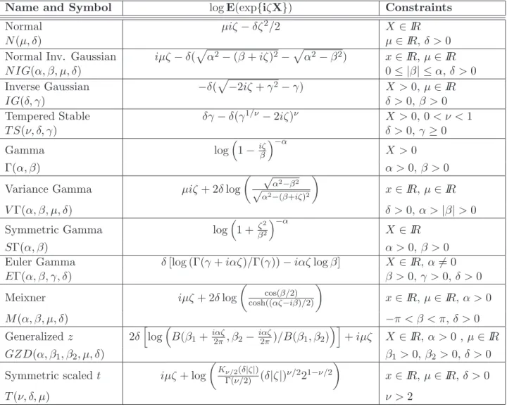
in several cases of interest and for models of wide applicability. Table (1) lists the cumulant function together with the parameter space and domain of some important examples by which OU processes with given marginal distribution can be constructed. Together with common distributions such as the Normal the t and the Gamma, we find some less known examples which find important applica-tions in financial and econometric data: the Normal Inverse Gaussian and the Inverse Gaussian, see Barndorff-Nielsen (1997, 1998), Rydberg (1997), Barndorff-Nielsen and Shephard (2001); the Tem-pered Stable, see Tweedie (1984) and Hougaard (1986), of which the Inverse Gaussian is a special case when κ = 1/2; the Variance Gamma, discussed in Madan and Seneta (1990) and Seneta (2004); the Symmetric Gamma, for which the reader is referred to Dufresne (1997), Kotz et Al. (2001, p. 179) and Steutel and van Harn (2004, p. 504); the Euler’s Gamma, see Grigelionis (2003); the Meixner, for which one can consult Schoutens and Teugel (1998) and Grigelionis (1999) and the Generalized
z, (Grigelionis, 2001) of which the Meixner can be seen as a special case. The elegant expression for
the ch.f. of the t-distribution has been provided by Heyde and Leonenko (2005). A general reference text on self-decomposable distributions and financial applications is Schoutens (2003).
3
Estimation
To enter the estimation problem, suppose that the marginal law of X(t) is a member of a family of
distributions indexed by a vector of parameters γ ∈ Γ ⊂ IRp−1 which is our estimation goal. More
generally, we may consider estimating the parameter vector θ ∈ Θ ⊂ IRp with θ = (γ0, λ)0 where
λ > 0 is the auto-regression parameter of the OU process.
Suppose we observe the process at equispaced time points 0 < t1 < · · · < . . . tnwith ∆ = tj−tj−1,
j = 1, . . . n, t0 = 0. In order to slightly simplify notation, denote the observation at time tj, X(tj),
by Xj. It follows from the discussion in Wolfe (1982) that, for self-decomposable distributions, a
discrete AR(1) process can be embedded into a continuous OU process. In our case, this amounts to say that the discretely observed OU process can be written as
Xj = e−λ∆Xj−1+ ε(λ)j , (3.12)
where the ε(λ)j ’s are i.i.d. random variables which are equal, in distribution, to the random variable
ε(λ)(1), hence their ch.f. has the form exp{κ(ζ) − κ(ζe−λ∆)}. Note that we will not be able to
distinguish between ∆ and λ so that we will actually consider estimation of, say, λ0 = λ∆ hence,
Name and Symbol log E(exp{iζX}) Constraints
Normal µiζ − δζ2/2 X ∈ IR
N (µ, δ) µ ∈ IR, δ > 0
Normal Inv. Gaussian iµζ − δ(pα2− (β + iζ)2−pα2− β2) x ∈ IR, µ ∈ IR
N IG(α, β, µ, δ) 0 ≤ |β| ≤ α, δ > 0
Inverse Gaussian −δ(p−2iζ + γ2− γ) X > 0, µ ∈ IR
IG(δ, γ) δ > 0, β > 0
Tempered Stable δγ − δ(γ1/ν− 2iζ)ν X > 0, 0 < ν < 1
T S(ν, δ, γ) δ > 0, γ ≥ 0 Gamma log ³ 1 −iζβ ´−α X > 0 Γ(α, β) α > 0, β > 0
Variance Gamma µiζ + 2δ log
µ √ α2−β2 √ α2−(β+iζ)2 ¶ x ∈ IR, µ ∈ IR V Γ(α, β, µ, δ) δ > 0, α > |β| > 0
Symmetric Gamma log
³ 1 +ζβ22
´−α
X ∈ IR
SΓ(α, β) α > 0, β > 0
Euler Gamma δ [log (Γ(γ + iαζ)/Γ(γ)) − iαζ log β] X ∈ IR, α 6= 0
EΓ(α, β, γ, δ) β > 0, γ > 0, δ > 0
Meixner iµζ + 2δ log
µ cos(β/2) cosh((αζ−iβ)/2) ¶ x ∈ IR, µ ∈ IR, α > 0 M (α, β, µ, δ) −π < β < π, δ > 0 Generalized z 2δ h log ³ B(β1+iαζ2π, β2−iαζ2π)/B(β1, β2) ´i + iµζ X ∈ IR, α > 0 , µ ∈ IR GZD(α, β1, β2, µ, δ) β1> 0, β2 > 0, δ > 0
Symmetric scaled t iµζ + log µ Kν/2(δ|ζ|) Γ(ν/2) (δ|ζ|)ν/221−ν/2 ¶ x ∈ IR, µ ∈ IR, δ > 0 T (ν, δ, µ) ν > 2
Table 1: Self-decomposable distributions and their Ch.f.. Γ(·) and B(·, ·) denote, respectively, Euler’s Gamma and Beta function while Kν(·) is the modified Bessel function of the third kind.
In this section we will slightly burden notation by introducing dependence on the parameters. So
we will write φγ(ζ) for E(eiζX) and, suppressing dependence on t, ϕθ(ζ) or ϕ(γ,λ)(ζ) for E(eiζε
(λ)(1)
) which, by Proposition 1, is φγ(ζ)/φγ(e−λζ); finally we write ψθ(ζ1, ζ2) for E[exp{i[ζ1X1+ ζ2X2]}.
The basic idea of the ch.f. estimation method is to minimize some (possibly weighted) distance function between an empirical estimator of the ch.f. and a model-based one. To enter in detail into the estimation problem, let us define first the empirical estimators of the ch.f. as
ψn(ζ1, ζ2) = n − 11 n−1 X j=1 exp{i[ζ1Xj+ ζ2Xj+1]}, (3.13) ϕn,λ(ζ) = n − 11 n−1 X j=1 exp{iζ[Xj+1− e−λXj]}. (3.14)
Note that ϕn,λ(ζ) = ψn(−e−λζ, ζ). Next define the quantities. Q1n(θ) = Z Z S |ψn(ζ1, ζ2) − ψθ(ζ1, ζ2)|2dW (ζ1, ζ2), (3.15) Q2n(θ) = Z S |ϕn,λ(ζ) − ϕθ(ζ)|2dW (ζ). (3.16)
The estimators are defined as the quantities minimizing the quadratic functions Q1
n(θ) or Q2n(θ), i.e.
ˆ
θ1 = arg min
θ∈ΘQ
1
n(θ), and θˆ2= arg min
θ∈ΘQ
2
n(θ). (3.17)
S denotes the region of integration and for convenience, according to the case at hand, may indicate
either a subset of IR or IR2. In the case of Q2
n(θ) which is one-dimensional, we may restrict attention
the the case S ⊂ IR+.
W (ζ1, ζ2) and W (ζ) are to be considered weighting functions which may serve different purposes
and characterize the estimation procedure. If they are chosen to be step functions we turn into a discrete set up which is much easier to implement from the computational point of view. Usually
one chooses a grid of points ζ1. . . ζm at which the ch.f. are evaluated and then minimizes a sum
instead of an integral. It is known that the choice of the grid of points has effect on the efficiency of the estimation procedure; Feuerverger and McDunnough (1981) show that, either in the i.i.d. or dependent case, using a weight given by the Fourier transform of the score and a grid sufficiently fine and extended the ch.f.-based estimation procedure is asymptotically equivalent to maximum likelihood estimation. In general the choice of an appropriate weight and grid may be impractical given the required quantities are seldom available explicitly and so one resorts to second best choices.
If we consider avoiding the choice of a grid and use a continuous version of Q1
n(θ) and Q2n(θ), the
choice of a proper weighting function is important in order to have a finite integral and for computa-tional reasons since the procedure becomes cumbersome to implement. Knight and Yu (2002) discuss
the use of an exponential weight (consider here Q2n(θ) for simplicity), i.e. dW (ζ) = exp{−ζ2}dζ, Epps
(2005), in the context of goodness of fit testing, suggests using dW (ζ) = (|ϕθ(ζ)|2/
R
|ϕθ(v)|2dv)dζ.
Both choices have the effect of damping out the persistent oscillations of |ϕn,λ(ζ) − ϕθ(ζ)|, as ζ → ∞
assuring finiteness of the integral but may not be optimal for efficiency considerations. Note that this last weighting scheme depends on θ, while our proposed weights do not. Under suitably regularity
conditions estimation based on Q1
n(θ) and Q2n(θ) is equivalent to an estimating equation approach
with weights depending on θ, for further details on equivalent approaches, see Knight and Yu (2002) and Jiang and Knight (2002).
Before discussing some of the properties of the above estimators let us note some of their features.
Q1n(θ) is the estimator based on the bivariate ch.f. discussed in Feuerverger and McDunnough (1981)
and Knight and Yu (2002), here we specialize it to the case of OU processes and give explicit solution for several cases of interest by exploiting Proposition 2.
Q2n(θ) is an estimator based on the ch.f. of the unobserved error term ε(λ) instead of that of the
observed Xj. It exploits the peculiar relation between the ch.f. of X and that of ε(λ) and can be
given explicit form by using Proposition 1, so it is applicable easily for all the models indicated in Table 1. Note that the auto-regression parameter λ is inserted into the empirical ch.f. estimator. Given the uniqueness of the Fourier-Stieltjes transformation, the amount of information contained in the ch.f. and the distribution function is the same. So this approach can be seen as an attempt to
substitute likelihood analysis on the sequence of i.i.d. errors ε(λ) which otherwise would be possible
essentially only in the Normal case.
This procedure however may have some drawbacks. First of all it may have identifiability
problems. Consider for example the case where the marginal distribution of X is N (0, σ2), then
φ(ζ) = exp{−σ2ζ2/2} and consequently, ϕ(ζ) = exp{−σ2(1 − e−2λ)ζ2/2} which is not identifiable
for all possible values of σ2 and λ. Next, the region of the λ values where Q2
n is minimized may
be quite large, note in fact that, for λ → ∞, we have that ϕθ(ζ) = ψθ(−e−λζ, ζ) → φγ(ζ) and
ϕn,λ→ (n − 1)−1P
jexp iζXj and hence one can achieve very small values of Q2n even with possibly
wrong values of λ, this may be a problem for numerical minimization routines, indeed some simula-tions we run indicated that in certain instances, the algorithm converges to large values of λ. Third, for large data set the minimization procedure is numerically cumbersome as it requires to evaluate
ϕn,λ(ζ) for each λ value in combination with each ζ value.
These features suggests that estimation of λ be undertaken exogenally; this makes the estimator considerably simpler to implement and computationally fast. We will then switch a little the problem,
considering estimation of the marginal parameters of X by minimizing Q2n(γ, ˆλ) wrt γ, where ˆλ is a
square root-consistent estimator of λ. We define then the estimators ˆ
γ = arg min γ∈ΓQ
2
n(γ, ˆλ). (3.18)
Note that this procedure exploits information on the structure of the process in order to estimate the marginal parameters and can lead to improved estimation procedures, as shown in Ghosh and Beran (2006) in the context of linear processes with long-range dependence.
The asymptotic theory for the estimators obtained from Q1
n(θ) can be straightforwardly obtained
from Knight and Yu (2002), under identifiability and regularity conditions stated there. Let θ0 =
(γ0, λ0) denote the true unknown parameter values.
Proposition 3. Under regularity conditions (see Knight and Yu (2002)), ˆθ1 is consistent for θ0 and
√ n ³ ˆ θ − θ0 ´ D → N¡0, B(θ0)−1A(θ0)B(θ0)−1 ¢ (3.19) where, for An(θ) = 12∂Q 1 n(θ)
∂θ , A(θ) = limn→∞n−1E [An(θ)An(θ)0] and B(θ) = Z Z S ∂ψθ(ζ1, ζ2) ∂θ ∂ψθ(ζ1, ζ2) ∂θ0 dW (ζ1, ζ2).
We need some more work to prove asymptotic results for ˆγ, in particular we need to add the
condition that EX1+δ< ∞ for some δ > 0 in order to have convergence under exogenous estimation
of λ.
Theorem 1. Under conditions A1 - A6 (see the Appendix), ˆγ is consistent for γ0 and
√ n (ˆγ − γ0)→ ND ¡ 0, B0(θ0)−1A0(θ0)B0(θ0)−1 ¢ . (3.20) where, for Gn(θ) = 12∂Q 2 n(γ,λ) ∂γ , A0(θ) = E [Gn(θ)Gn(θ)0] and B0(θ) = Z S ∂ ϕγ,λ(ζ) ∂γ ∂ ϕγ,λ(ζ) ∂γ0 dW (ζ).
Remark 2. As we will see in the Appendix, computation of A0(θ) does not require to consider covariance terms and hence turns out to be considerably simpler wrt A(θ).
4
Applications
4.1 The Normal Inverse Gaussian OU process
As a first example of application consider the NIG-OU process introduced by Barndorff-Nielsen (1998). From Table 1 we see that the marginal law of the process is characterized by 4 parameters which makes it quite a flexible distribution. Here, δ is a scaling and µ a location parameter, whereas
β is an asymmetry parameter and the quantities α ± β determine the heavyness of the tails. Here
we consider the case with µ = 0. The law governing the BDLP of the NIG-OU process has been analitically derived by Barndorff-Nielsen (1998), in particular the BDLP is composed by three inde-pendent L´evy processes. Using simulation-based techniques for this case may turn an unwieldly task since one needs to (approximately) simulate three separate L´evy processes with jumps. Instead, it turns out to be quite simple to apply the procedure discussed here. In fact, from the univariate ch.f. of Table 1, for µ = 0, Proposition 1 and Proposition 2 obtain that
ϕθ(ζ) = exp ½ −δ(pα2− (β + iζ)2− q α2− (β + ie−λζ)2 ¾ (4.21) and ψθ(ζ1, ζ2) = exp{−δ(pα2− β2−pα2− (β + iζ 2)2+ q α2− (β + ie−λζ 2)2 − q α2− (β + i(ζ 1+ e−λζ2))2}. (4.22)
This example will be taken as an occasion to perform a small simulation study to compare
the estimation procedures based on Q1
n(θ), Q2n(γ, ˆλ) and moment-based estimators; the computing
equations for these in the NIG case can be found, for example in Karlis (2002). We will consider an OU process with λ = 1 and a N IG(α = 2, β = 1, δ = 1) marginal distribution. Several sample paths from such a process will be generated as suggested in Taufer and Leonenko (2008); it will be assumed that the sampling interval of the process is unity, i.e. ∆ = 1 and the case where dW (ζ) is a step function will be considered, turning in this way into a discrete estimation framework. The sampling
intervals of the ch.f. will also be constant and set to ζj− ζj−1 = 0.05, j = 1, . . . m. The choice of
the step size maybe quite important in order to minimize effectively the distance of the empirical ch.f. and the model one. Feuerverger and McDunnough (1981) discuss optimizing procedures in order to obtain, for fixed sampling size of the ch.f., either an optimal fixed step or optimal sampling
points ζ1, . . . , ζm. As far as the number m of the sampling points, it was found to be very effective
the heuristic approach of plotting |φ(ζ)|2 against ζ and choose m, given the step, which samples the
empirical ch.f. until it is sensibly different from 0. According to different cases, some calibration would be desirable, however a large simulation study is out of purpose here. The results of the simulations are in line with those of Feurverger and McDunnough (1981).
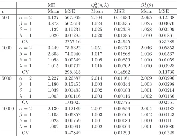
Table (2) gives the sample mean and the mean square error (MSE) of the moment-based
estima-tors, indicated as ME, those based on Q1
n(θ) and those based on Q2n(γ, ˆλ). The preliminary estimator
of λ in the case of Q2
n(γ, ˆλ) is the standard auto-correlation estimator between Xj and Xj+1which is
connected with the maximum likelihood estimator of λ in the Normal case, this estimator has been used also in conjunction with ME. The results are based on 1000 replications of samples of sizes ranging from 500 to 10000. For each sample size, we reported in the line indicated with OV (overall variability), the algebric sum of the elements of the variance-covariance matrix of the estimators
ME Q2
n(η, ˆλ) Q1n(θ)
n Mean MSE Mean MSE Mean MSE
500 α = 2 6.127 567.969 2.104 0.14983 2.095 0.12538 β = 1 4.878 562.614 1.024 0.03635 1.025 0.03070 δ = 1 1.122 0.10231 1.025 0.02358 1.028 0.02599 λ = 1 1.020 0.01285 1.020 0.01285 1.070 0.01861 OV 2257.16 0.34945 0.31289 1000 α = 2 3.449 75.5322 2.051 0.06179 2.046 0.05353 β = 1 2.303 74.0240 1.017 0.01868 1.016 0.01567 δ = 1 1.093 0.00549 1.009 0.00859 1.010 0.01059 λ = 1 1.015 0.00702 1.015 0.00702 1.010 0.00928 OV 298.813 0.14862 0.13735 5000 α = 2 2.227 0.26587 2.014 0.01161 2.009 0.00996 β = 1 1.180 0.15455 1.003 0.00344 1.003 0.00298 δ = 1 1.039 0.01485 1.002 0.00183 1.001 0.00214 λ = 1 1.003 0.00116 1.003 0.00116 1.002 0.00166 OV 1.03025 0.02775 0.02551 10000 α = 2 2.130 0.12189 2.007 0.00556 2.004 0.00488 β = 1 1.103 0.06852 1.003 0.00169 1.002 0.00143 δ = 1 1.023 0.00759 1.001 0.00089 1.000 0.00111 λ = 1 1.002 0.00064 1.002 0.00064 1.001 0.00080 OV 0.47849 0.01299 0.01229
Table 2: Sample Mean and MSE of estimates based on simulated data of NIG(2,1,1)-OU process with λ = 1, 1000 iterations.
corrected by the bias terms; it is an attempt to give a measure of the overall performance of each method in terms of M SE.
Placing attention on the results, we see that ME are highly unreliable for α and β for smaller sample sizes and the bias remains quite high even in large sample sizes. Estimation of δ and λ is much more reliable. Turning to the estimators based on the ch.f. we see both perform much better for all sample sizes, with very small bias even at smaller sample sizes. Overall it seems that the
procedure based on Q1
n(θ) is slightly superior even if differences are very small. At the level of single
parameters Q1n(θ) is generally better for α and β whicle Q2n(γ, ˆλ) is generally better for δ and λ.
Evidence seems to indicate that estimation of λ may be better if taken exogenally.
4.2 GDP growth rates
As an application to real data we consider estimation of the sequence of quarterly US GDP growth rates. It is defined as the logarithm difference of the real (in 2000 constant dollars), seasonally adjusted US GDP sequence from the first quarter of 1947 to the second quarter of 2007 for a total of 241 observations. The same sequence, but up to 2000, has been studied by Chan et al. (2004), together with other economic series with non-Normal errors. Chan et al. (2004) find that an AR(1) model fits well to the data although they decidedly show non-Normality, they provide bootstrap procedures for quarterly intervals forecasts. Here, without the pretention to fully analyze the data
set, and building on Chan et al. (2004), we proceed by adapting a discretely observed OU process with NIG marginal distribution which seems a good candidate given its flexibility in modelling data with asymmetry and/or heavier tails than the Normal. A quick moment estimates of the data reveals a slight asymmetry with a coefficient of 0.14 and an excess kurtosis of 1.37. Figure 1a shows a Q-Q plot of the data against a NIG model with α = 0.3468, β = 0.0500, µ = 2.8950, δ = 5.5160, λ = 1.1110, the fit is remarkably good for experimental data, the parameter values have been determined by the
two step Q2
n procedure. Figure 1b shows the plot of |ϕn,ˆλ(ζ)|2 and |ϕθˆ(ζ)|2 against ζ. One can note
that adherence of the ch.f. of is remarkably good in all cases.
æ æ æ ææ æææ æææææ æææ æææææææææ æ æææææææ æææææææææææææææææææææææææææææææææææææææææææææææææææææææææææææææææææææææææææææææææææææææææææææææææææææææææææææææææææææææææææææææææææææææææææææææææææææææææ ææææææææææææææææææææææææææææææææææææ æææææææææ ææ ææ ææ æ æ æ æ -5 5 10 15 20 -10 -5 5 10 15 (a) 0.0 0.2 0.4 0.6 0.8 1.0 0.2 0.4 0.6 0.8 1.0 (b)
Figure 1: a) Q-Q plot of the data against a N IG(0.3468, 0.0500, 2.8950, 5.5160) distribution; b) Plot of |ϕn,ˆλ(ζ)|2 (solid), |ϕ
ˆ
θ(ζ)|2, ˆθ from Q1n, (dotted) and |ϕγ,ˆˆλ(ζ)|2, ˆγ from Q2n, (dashed) against ζ, ˆλ
auto-correlation estimator.
5
An extension to Stochastic volatility models
Consider the following asset return process with stochastic conditional volatility of the log-asset price
S(t)
dS(t) = {µ + βX(t)}dt +pX(t)dN (t) (5.23) where X(t) is a non-negative OU process as defined in (1.1) and N (t) is a standard Brownian motion independent of X(t), µ is a drift and β is a risk premium parameter. This model was introduced in Barndorff-Nielsen and Shephard (2001) with the aim of modelling stylized features of financial markets while maintining analytical tractability. The positive OU process X(t), with no Gaussian component, moves entirely by jumps and decays exponentially between two jumps
while S(t) remains continuous; to introduce discontinuities one can introduce a L´evy component in
equation (5.23). Suppose we observe the process S(t) at fixed time instants t0 < t1 < · · · < tm
and define ∆S(tj) = S(tj) − S(tj−1), then ∆S(tj)|∆x∗(tj) ∼ N (µ(tj− tj−1) + βx∗(tj), x∗(tj)) where
∆X∗(t
j) = X∗(tj) − X∗(tj−1) and X∗(tj) =
Rtj
0 X(s)ds is the integrated volatility; ∆x∗(tj) is termed
actual volatility. The terms ∆S(tj)|∆x∗(tj) j = 1 . . . n are conditionally independent and we note
that the distribution of ∆S(tj) will be a location scale mixture of normals. By an appropriate design
of the stochastic process for X(t) one can allow aggregate returns to be heavy tailed, skewed and exhibit volatility clustering. Following the discussion of Section 2, typical choices for the marginal distribution of X(t) are the Inverse Gaussian and Gamma distributions, alternatively one may model directly the BDLP of X(t) obtaining a variety of models which can adapt very well to practical situations. For further details on these models one can refer to Barndorff-Nielsen and Shephard (2001, 2003).
Estimating the parameters of a continuous stochastic volatility model is difficult owing to the inability to compute the appropriate likelihood function. Model-based estimation approaches are based on MCMC methods and references to recent related works are those of Barndorff-Nielsen and Shephard (2001), Gander and Stephens (2006, 2007) Griffin and Steel (2006). Alternatively one might consider non-model-based estimation approaches which exploits realized volatility, i.e. use the existence of high-frequency intraday data to directly estimate moments of integrated volatility, which was introduced by Barndorff-Nielsen and Shephard (2002), for extensions on this approach and further references to recent works one can consult Woerner (2007).
Here we sketch shortly how we could implement ch.f. based estimation. This can be done quite easily as explicit expressions may be derived with little work. Asimptotic properties of these estimators can be obtained by the method discussed in Knight et al. (2002) which has studied ch.f. based estimation of a stochastic volatility model based on a Gaussian volatility model.
Theorem 2 obtains the joint characteristic function of the increments of the stochastic volatility
process in term of the cumulant generating function of the BDLP `Z(1) of X(t), this exists in closed
form for key cases such as the Inverse Gaussian and the Gamma and allows to obtain results in closed form solution.
Theorem 2. Let k(ζ) = log Ee−ζ `Z(1), the joint characteristic function of ∆S(t
1), . . . ∆S(tm) is exp{iµ m X j=1 ζj(tj− tj−1)} exp{λ Z ∞ 0 k(Je−λs)ds} exp{λ m X l=0 Z tl tl−1 k(Hl(s))ds}, (5.24) where J = m X j=1 µ 1 2ζ 2 j − iβζj ¶ ελ(tj−1, tj), (5.25) Hl(s) = m X j=l+1 µ 1 2ζ 2 j − iβζj ¶ ελ(tj−1, tj)eλs+ II(l>0) µ 1 2ζ 2 l − iβζl ¶ ελ(0, tl− s). (5.26)
With ελ(u, v) = 1λ(e−λu− e−λv) and the convention that t−1 = 0 and
Pm
5.1 Marginal models for X(t)
To get more specific in our modelling framework we present two important models for the marginal distribution of the volatility process which allow to obtain a variety of behaviours for the process
S(t).
The expressions for the ch.f. we have provided are in terms of k(ζ) = log E{exp(−ζ `Z(1))} hence
one can model directly from the BDLP if has a direct expression for this. Alternatively if one prefers modelling by first specifying a marginal distribution for the process X(t) and exploiting the relation
`
κ(ζ) = ζ∂κ(ζ)
∂ζ (5.27)
and the fact that k(ζ) = κ(−iζ).
A first important model for X is the Tempered Stable, see Table 1, i.e. X ∼ T S(ν, δ, γ). When
ν = 1/2 we have the important sub-case of the Inverse Gaussian distribution. For the TS case,
exploiting (5.27) we obtain
k(ζ) = −2ζνδ2ν(γ2+ 2ζ)ν−1. (5.28)
For this case, the ch.f. of ∆S(t1), . . . , ∆S(tm) can be given explicit form in terms of hypergeometric
series. Here, to avoid large expressions we report the IG case for m = 1, let AT denote the ArcTanh
function and tj− tj−1= ∆, we have
C{ζ‡∆S(tj)} = 2δ ³ ζ2 2 − iζβ ´ · AT µ (B−1)q1 +2(1−e−λ∆)(ζ2/2−iζβ) γ2λ ¶ − AT (B−1) ¸ λγB (5.29) where B = q
1 +2(ζ2/2−iζβ)γ2λ . As we see, although cumbersome, the above function is
straightfor-wardly applicable in numerical procedures.
Another important case is the Generalized Inverse Gaussian model, which we denote by X ∼
GIG(ν, δ, γ), with δ ≥ 0, γ > 0 if ν > 0, δ > 0, γ > 0 if ν = 0 and δ > 0, γ ≥ 0 if ν < 0. For details
see Eberlein (2001) and Barndorff-Nielsen and Shephard (2001b); this model has ch.f.
φ(ζ)GIG(ν,δ,γ) = µ γ2 γ2− 2ζ ¶ν/2 Kν(δ p γ2− 2ζ) Kν(δγ) . (5.30)
where Kν(x) denote the modified Bessel function of the third kind. The appropriate form of k(ζ)
for the GIG model, not shown here, can be recovered by (5.27). Note that
∂Kν(x) ∂x = −
1
2(Kν−1(x) + Kν+1(x)). (5.31)
In the limiting case ν > 0, δ = 0 it reduces to the density of a Gamma distribution Γ(γ2, ν/2);
for ν < 0, γ = 0 one gets those of a reciprocal Gamma distribution. For the Gamma case we have the simple form
k(ζ) = νζ
Notably the IG distribution is common either to the TS and to the GIG distribution, being
IG(δ, γ) ∼ T S(1/2.δ, γ) ∼ GIG(−1/2, δ, γ).
In the cases where an explicit form of the ch.f. of the process (5.23) cannot be obtained, it appears that (5.24) is well suited for numerical integration. Also, by using the same techniques discussed in Theorem 2 one can provide expressions for the ch.f. of stochastic volatility models with leverage and where superpositions of OU processes are used to model volatility. It appears that a thorough investigation of these models would require much additional work which seems suitable for a separate paper. 0.05 0.06 0.07 0.08 0.09 0.5 1 1 1.5 1.5 2 2 2.5 2.5 3 3 3.5 3.5 0.5 1.0 1.5 2.0 2.5 3.0 3.5 4.0 1 2 3 4 ∆ Γ (a) 0.05 0.06 0.06 0.07 0.07 0.08 0.08 0.09 0.09 0.5 0.5 1 1 1.5 1.5 2 2 2.5 2.5 3 3 3.5 4 4.5 0.5 1.0 1.5 2.0 2.5 3.0 3.5 4.0 0 1 2 3 4 ∆ Λ (b)
Figure 2: Contour plots of the objective function for model (5.23) with X(t) following and IG-OU process with δ = 2, γ = 1, λ = 0.01. Lenght of series n=2500. a) (δ, γ); b) (δ, λ).
Here we give a brief report on some results with simulated data by estimating the paramters for a series of lenght 2500 from model (5.23) with µ = β = 0 and where X(t) follows and IG(2, 1) OU
process with λ = 0.01. Figure 2 provides the contour plots of the objective function based on Q1n(θ)
obtained by using (5.24) with m = 2 and the empirical estimator ψn(ζ1, ζ2) with 400 pairs (ζ1, ζ2)
generated from two independent N (0, 3) distributions.
Although the plots represent a single simulation, it appears that the objective function has quite a regular behaviour with very low values in the neighborhood of the true values of the parameters.
6
Appendix: Proofs
Proof of Proposition 1. Let II denote the indicator function; let f (t) = e−λ(t−s)II(0,t](s) and apply formula (2.7) to obtain log ϕt(ζ) = λ Z ∞ 0 ` κ ³ e−λ(t−s)II(0,t](s)ζ ´ ds = λ Z t 0 e−λ(t−s)ζ κ0 ³ e−λ(t−s)ζ ´ ds = κ(ζ) − κ(ζe−λt)
from which the result follows.
Proof of Proposition 2. From (2.10), for t2 > t1, write
log ψ(ζ1, ζ2) = λ Z IR ` κ X2 j=1 ζjII(tj>s)(s)e−λ(tj−s) ds = λ Z t1 −∞ ` κ X2 j=1 ζje−λ(tj−s) ds + λ Z t2 t1 ` κ ³ ζ2e−λ(t2−s) ´ ds
next use, as in Proposition 1, the relation `κ(ζ) = ζκ0(ζ) to formally integrate and obtaining the
result.
The following technical result will be needed in the proof of Theorem 1.
Lemma 3. Let λ∗ p→ λ as n → ∞ and assume that E|X|1+δ < ∞ for some δ > 0. Then
i) ϕn,λ∗(ζ) →p ϕθ(ζ), and ii) ∂ ∂λϕn,λ(ζ) ¯ ¯ λ=λ∗ p → ∂ ∂λϕθ(ζ), (6.33) where ∂ ∂λϕθ(ζ) = iζe−λϕθ(ζ)E(X).
Proof of Lemma 3. Denote by op(1) a quantity converging in probability to 0 as n → ∞ and recall
that |eiu| = 1. To prove i) we first prove that we can simply consider the empirical estimator of the
ch.f. evaluated at λ instead of λ∗. Note that
¯ ¯ ¯ ¯ ¯ϕn,λ∗(ζ) − ϕn,λ(ζ) ¯ ¯ ¯ ¯ ¯= ¯ ¯ ¯ ¯ ¯ 1 n − 1 n−1 X j=1 ³
eiζ(Xj+1−e−λ∗Xj)− eiζ(Xj+1−e−λXj)
´¯¯¯ ¯ ¯ ≤ 1 n − 1 n−1 X j=1
|eiζXj+1||e−iζλXj||(eiζXj(e−λ−e−λ∗)− 1|
≤ 22−δ¯¯e−λ− e−λ∗¯¯δ |ζ|δ n − 1 n−1 X j=1 |Xj|δ = op(1).
Here the last inequality is obtained from |eiu− 1| ≤ 22−δ|u|δ, see, for example, Sen and Singer (1993,
formula 1.4.59). Note that for this result to hold we only require that E|X|δ< ∞.
Part ii) can be proved by the same devices. Note first that ¯ ¯ ¯ ¯ ¯ ∂ ∂λϕn,λ(ζ) ¯ ¯ λ=λ∗− ∂ ∂λϕn,λ(ζ) ¯ ¯ ¯ ¯ ¯ = ¯ ¯ ¯ ¯ ¯ 1 n − 1 n−1 X j=1 ³
iζe−λ∗Xjeiζ(Xj+1−e
−λ∗X j)− iζe−λX jeiζ(Xj+1−e −λX j) ´¯¯ ¯ ¯ ¯ ≤ |e−λ∗− e−λ| |ζ| n − 1 n−1 X j=1 |Xj| + 22−δ ¯ ¯e−λ− e−λ∗¯¯δ |ζ|δ n − 1 n−1 X j=1 |Xj|1+δ = op(1).
Next, to obtain the result we note that from Sørensen (1999, Theorem 3.2)
iζe−λ 1 n − 1 n−1 X j=1 eiζ(Xj+1−e−λXj)X
j a.s.→ iζe−λE(eiζ(Xj+1−e
−λX
j)X
j) (6.34)
and, by independence of Xj+1− e−λXj and Xj, E(eiζ(Xj+1−e
−λX
j)X
j) = ϕθ(ζ)E(X).
Proof of Theorem 1. We need the following regularity conditions and assumptions:
A1 The parametrization used brings to an identifiable problem, i.e. ϕθ0(ζ) 6= ϕθ(ζ) if θ0 6= θ; Θ
is a compact set and θ0 ∈ Int(Θ).
A2. ϕθ(ζ) is twice continuously differentiable in θ.
A3 Gn(γ, λ) = 12∂Q
2
n(γ,λ)
∂γ , ∂λ∂ Gn(γ, λ) and ∂γ∂ Gn(γ, λ) are W -integrable functions over Θ.
A4. The matrix B0(θ) defined in Theorem 1 is a W -integrable function over Θ and is of full rank
at θ0.
A5. For a δ > 0, E|X|1+δ < ∞.
A6. ˆλ is a√n-consistent estimator of λ.
For the proof of consistency, under E(Xδ) < ∞ and λ∗ → λ we have from Lemma 3.i), thatp
|ϕn,λ∗(ζ) − ϕn,λ(ζ)| = op(1) and noting that ϕn,λ(ζ) is an empirical ch.f. based on i.i.d. observations,
consistency follows by standard arguments by A1, A2 and A3.
Next, to prove asymptotic normality, by expanding Gn(ˆγ, ˆλ) around γ we have, for |γ∗− γ| ≤
|ˆγ − γ|, √ nGn(ˆγ, ˆλ) = √ nGn(γ, ˆλ) + √ n(ˆγ − γ) ∂ ∂γGn(γ, ˆλ) ¯ ¯ γ=γ∗. (6.35)
Asymptotic normality of√n(ˆγ−γ) will follow if we prove that: a)√nGn(γ, ˆλ), with λ playing the role
of nuisance parameter, is asymptotically Normal and b) ∂γ∂ Gn(γ, ˆλ)
¯ ¯ γ=γ∗∂γ∂0Gn(γ, ˆλ) ¯ ¯ γ=γ∗ → B0(θ)
where B0(θ) is defined in A4.
To prove a), note that, by a further Taylor expansion around λ, with |λ∗− λ| ≤ |ˆλ − λ| we have
√ nGn(γ, ˆλ) = √ nGn(γ, λ) + √ n(ˆλ − λ) ∂ ∂λGn(γ, λ) ¯ ¯ λ=λ∗, (6.36)
To ease a little notation, let ∂λ∂ ϕn,λ(ζ)¯¯λ=λ∗ = ˙ϕn,λ∗(ζ), then we have ∂ ∂λGn(γ, λ) ¯ ¯ λ=λ∗ = Z S (Re ˙ϕn,λ∗(ζ) − Re ˙ϕγ,λ∗(ζ)) ∂ ∂γϕγ,λ∗(ζ)dW (ζ)+ + Z S (Re ϕn,λ∗(ζ) − Re ϕγ,λ∗(ζ)) ∂ ∂γϕ˙γ,λ∗(ζ)dW (ζ) + Im (6.37)
where Im denotes the same expression of the r.h.s. of the above formula but with Re replaced by
Im. By dominated convergence theorem we have ˙ϕγ,λ∗(ζ) = iζe−λ ∗
E[Xjexp{iζ(Xj+1− e−λ
∗
Xj}]
which, using uniform continuity of the ch.f. and the same devices used in Lemma 1, converges
in probability to iζe−λϕ
γ,λ(ζ)E(X). Using this result, Lemma 3.ii) and A3 we can prove that
∂
∂λGn(γ, λ)
¯ ¯
λ=λ∗ converges in probability to 0 and since, by assumption,
√
n(ˆλ − λ) = Op(1), we
have that the asymptotic distributions of √nGn(γ, ˆλ) and
√
nGn(γ, λ) are the same. Namely, since
Gn(γ, λ) is a sum of i.i.d. random variables, the standard central limit theorem obtains
√
nGn(γ, λ) →D N (0, A0(θ0)) (6.38)
where A0(θ
0) = EGn(γ, λ)Gn(γ, λ)0. As far as part b) is concerned, note that we have
∂ ∂γGn(γ, λ) = Z S (Re ϕn,λ(ζ) − Re ϕγ,λ(ζ))∂γ∂γ∂ 0ϕγ,λ(ζ)dW (ζ)+ + Z S ∂ ∂γRe ϕγ,λ(ζ) ∂ ∂γRe ϕγ,λ(ζ)dW (ζ) + Im. (6.39)
Again, we can use the results of Lemma 1 and dominated convergence to get the desird result. The proof can be completed by standard arguments as in, for example, Feuerverger and McDunnough (1981).
Proof of Theorem 2. The characteristic function of E exp{iζR0∞f (t)dS(t)} for a general positive
function f (u) can be obtained straightforwardly from Barndorff-Nielsen and Shephard (2001, formula
36); there H(s) = R0∞{12ζ2f2(u + s) − iβζf (u + s)}e−λudu and J = H(0). To obtain our result,
we need to set ζ = 1 and plug in f (s) = Pmj=1ζjII(tj−1,tj](s). Note first of all that, since (tj−1, tj]
and (tj0−1, tj0] do not overlap, for j 6= j0, then f2(s) = Pmj=1ζj2II(t
j−1,tj](s), this allows to obtain
straightforwardly expression (5.25). To obtain the expression for H(s) we write
II(tj−1,tj](u + s) = II(tj−1−s,tj−s](u)II(0,tj−1](s) + II(0,tj−s](u)II(tj−1,tj](s) (6.40) to obtain H(s) = m X j=1 µ 1 2ζ 2 j − iβζj ¶ h ελ(tj−1− s, tj− s)II(0,tj−1](s) + ελ(0, tj − s)II(tj−1,tj](s) i . (6.41)
In order to computeRk(H(s))ds it is convenient to separate the components of H(s) over the disjoint
intervals (tj−1, tj] and proceed to integrate over separate regions. To this end, write II(0,tj−1](s) =
Pj−1
7
Bibliography
Baran, S., Pap, G., van Zuijlen, M. C. A. (2003). Estimation of the mean of stationary and nonsta-tionary Ornstein-Uhlenbeck processes and sheets. Comput. Math. Appl. 45, 563-579.
Barndorff-Nielsen, O.E. (1997). Normal inverse Gaussian distributions and stochastic volatility mod-elling. Scand. J. Statist. 24, no. 1, 1-13.
Barndorff-Nielsen, O.E. (1998). Processes of Normal Inverse Gaussian type. Finance and Stochastics 2, 41-68.
Barndorff-Nielsen, O. E. (2001). Superposition of Ornstein-Uhlenbeck type processes. Theory
Probab. Appl. 45, no. 2, 175-194. Translated from Teor. Veroyatnost. i Primenen. 45 (2000),
no. 2, 289-311;
Barndorff-Nielsen, O.E, Jensen, J.L, Sørensen, M. (1998). Some stationary processes in discrete and continuous time. Adv. Appl. Prob. 30 (4), 989-1007.
Barndorff-Nielsen, O.E., Shephard, N. (2001). Non-Gaussian Ornstein-Uhlenbeck-based models and some of their uses in financial economics. J. R. Stat. Soc. Ser. B Stat. Methodol. 63 , no. 2, 167-241.
Barndorff-Nielsen, O.E., Shephard, N. (2002). Econometric analysis of realized volatility and its use in estimating stochastic volatility models. J. R. Stat. Soc. Ser. B Stat. Methodol. 64 , no. 2, 253-280.
Barndorff-Nielsen, O.E., Shephard, N. (2003). Integrate OU processes and non-Gaussian OU-based stochastic volatility models. Scand. J. Stat., 30, 277-295.
Barndorff-Nielsen, O. E., Leonenko, N. N. (2005). Spectral properties of superpositions of Ornstein-Uhlenbeck type processes. Methodol. Comput. Appl. Probab. 7, no. 3, 335-352.
Dufresne, D. (1997). Algebraic properties of Beta and Gamma distributions, and applications. Adv.
Appl. Math. 20, 285-299.
Feuerverger, A. (1990). An efficiency result for the empirical characteristic function in stationary time-series models. Canad. J. Statist. 18, no. 2, 155-161.
Feuerverger, A. and McDunnough, P. (1981). On some fourier methods for inference. J. Amer. Stat.
Assoc. 76, 379-387.
Florens-Landais, D., Pham, H. (1999). Large deviations in estimation of an Ornstein-Uhlenbeck model. J. Appl. Probab. 36, 60-77.
Gander, M.P.S., Stephens, D.A. (2007a). Stochastic volatility modelling in continuous time with general marginal distributions: inference, prediction and model selection. J. Stat. Plann. and Infer. 137, 3068-3081.
Gander, M.P.S., Stephens, D.A. (2007b). Simulation and inference for stochastic volatility models driven by L´e vy processes. Biometrika 94, no.3, 627-646.
Ghosh, S. and Beran, J. (2006). On estimating the cumulant generating function of linear processes.
Ann. Inst. Statist. Math. 58, no. 1, 53-71.
Gloter, A. (2001). Parameter estimation for a discrete sampling of an integrated Ornstein-Uhlenbeck process. Statistics 35, 225–243.
Griffin, J.E., Steel, M.F.J. (2006). Inference with non-Gaussian Ornstein-Uhlenbeck processes for stochastic volatility. J. Econometics 134, 605-644.
Grigelionis, B. (1999). Processes of Meixner type. Liet. Mat. Rink. 39, no. 1, 40-51; translation in
Lithuanian Math. J. 39 (1999), no. 1, 33-41.
Grigelionis, B. (2001). Generalized z-distributions and related stochastic processes. Liet. Mat. Rink. 41, no. 3, 303-319; translation in Lithuanian Math. J. 41 (2001), no. 3, 239-251.
Grigelionis, B. (2003). On the self-decomposability of Euler’s Gamma function. Liet. Mat. Rink. 43, no. 3, 359-370; translation in Lithuanian Math. J. 43 (2003), no. 3, 295-305.
Heyde, C.C.; Leonenko, N. (2005). Student processes. Adv. Appl. Prob. 37, 342-365.
Hougaard, P. (1986). Survival models for heterogeneous populations derived from stable distribu-tions. Biometrika 73, 387-396.
Jiang, G.J.; Knight, J.L. (2002). Estimation of continuous-time processes via the empirical charac-teristic function. J. Bus. Econom. Statist. 20, no. 2, 198-212.
Jongbloed, G.; van der Meulen, F.H. (2006). Parametric estimation for subordinators and induced OU processes. Scand. J. Statist. 33, no. 4, 825-847.
Jongbloed, G.; van der Meulen, F. H.; van der Vaart, A. W. (2005). Nonparametric inference for Lvy-driven Ornstein-Uhlenbeck processes. Bernoulli 11, no. 5, 759-791.
Jurek, Z.J. and Vervaat, W. (1983). An integral representation for self-decomposable Banach space random variables. Zeit. Wahrsch. ver. Gebiete 62, 247-262.
Knight, J.L. and Satchell, S.E. (1997). The cumulant generating function estimation method.
Econo-metric Theory 13, 170-184.
Knight, J.L. and Yu, J. (2002). Empirical characteristic function in time series estimation.
Econo-metric Theory 18, 691-721.
Knight, J.L.; Satchell, S.E.; Yu, J. (2002). Estimation of the stochastic volatility model by the empirical characteristic function method. Aust. N. Z. J. Stat. 44, no. 3, 319-335.
Kotz, S., Kozubowski, T. J., Podg´orski, K. (2001). The Laplace Distributions and Generalizations. Birkh¨auser, Boston.
Madan, D.B. and Seneta, E. (1987). Simulation of estimates using the empirical characteristic function International Statistical Review 55, 153-161.
Madan, D.B., Seneta, E. (1990). The VG model for share market returns. J. Bus. 63, 511-524. Neumann, M.J. and Reiss, M. (2008). Nonparametric estimation for L´evy processes from low-frequency observations. Preprint.
Pap, G., van Zuijlen, M. C. A. (1996). Parameter estimation with exact distribution for multidi-mensional Ornstein-Uhlenbeck processes. J. Multiv. Anal. 59, 153-165.
Roberts, G.O.; Papaspiliopoulos, O.; Dellaportas, P. (2004). Bayesian inference for non-Gaussian Ornstein-Uhlenbeck stochastic volatility processes. J. R. Stat. Soc. Ser. B Stat. Methodol. 66, no. 2, 369-393.
Rydberg, H (1997). The Normal Inverse Gaussian L´evy process: simulation and approximation.
Communications in Statistics - Stochastic Models 13 (4), 887-910.
Sato, K.I.(1999). Levy Processes and Infinitely Divisible Distributions. Cambridge University Press, Cambridge.
Schoutens, W., Teugels, J.L. (1998). L´evy processes, polynomials and martingales. Special issue in honor of Marcel F. Neuts. Comm. Statist. Stochastic Models 14, no. 1-2, 335-349.
Schoutens, W. (2003). L´evy Processes in Finance. Wiley, Chicester.
Sen, P.K. and Singer, J.M. (1993). Large Sample Methods in Statistics. Chapman & Hall, London. Seneta, E. (2004) Fitting of Variance-Gamma model to financial data. J. Appl. Probab. 41 A, 177-187.
Sørensen, M. (1999). On asymptotics of estimating functions. Braz. J. Probab. Stat. 13, no. 2, 111-136.
Steutel, F. W., van Harn, K. (2004). Infinite Divisibility of Probability Distributions on the Real
Line. Marcel Dekker, New York.
Taufer, E., Leonenko, N. (2008). Simulation of Levy-driven Ornstein-Uhlenbeck processes with given marginal distribution. Computational statistics & data analysis, Articles in press.
Todorov, V., Tauchen, G. (2006). Simulation methods for Lvy-driven continuous-time autoregressive moving average (CARMA) stochastic volatility models. J. Bus. Econom. Statist. 24, no. 4, 455-469. Tweedie, M.C.K. (1984). An index which distinguishes between some important exponential families. In Statistics: Applications and New Directions: Proc. Indian Statistical Institute Golden Jubilee
International Conference (ed. J. Ghosh and J. Roy), pp. 579-604.
Woerner, J.H.C. (2004) Estimating the skewness in discretely observed L´evy processes. Econometric
Theory 20, 927-942.
Woerner, J.H.C. (2007)Inference in L´evy-type stochastic volatility models. Adv. Appl. Prob. 39,
531-549.
Wolfe, J. (1982). On a continuous analogue of the stochastic difference equation Xn= ρXn−1+ Bn.