ON SOME DESCRIPTIVE AND PREDICTIVE METHODS FOR
THE DYNAMICS OF CANCER GROWTH
Iulian T. Vlad
Department of Mathematics, University Jaume I of Castell´on, Spain Jorge Mateu
Department of Mathematics, University Jaume I of Castell´on, Spain Elvira Romano1
Department of Political Science Jean Monnet, Second University of Naples, Caserta, Italy
1. Introduction
The evolution in time of some objects is the subject of study of many researchers worldwide. Special attention has been given to cancer, and a way to understand this disease is to know how it evolves over time. We can find, in reading, many studies about mathematical modeling of tumors, which attempt to predict the growth of tumors from a mathematical point of view. See, for example, Bramson and Griffeath (1981), Cressie (1991), Qi et al. (1993) , Lee and Cowan (1994) or Kansal et al. (2000). The development of tumor models is important as they offer a way to better understand the kinetic growth of malignant tumors which may lead to the development of successful treatment strategies. In present day societies, cancer is a widely spread disease that affects a large proportion of the human population, and many research teams are developing algorithms to help medics to understand this disease. In particular, tumor growth has been studied from different viewpoints and different mathematical models have been proposed. There is an increasing interest in observing the dynamics of cancer tumors, and in developing and implementing new methods and algorithms for prediction of tumor growth. These tools help physicians to better understand and treat these type of diseases. Using a prediction method and comparing with the real evolution, a physician can note if the prescribed treatment has the desired effect, and according to this, if necessary, to take the decision of intervention. We thus are interested in analyzing the spatio-temporal dynamics of brain tumors coming from objects that are originally processed from computer tomography images, and can be depicted as a collection of image pixels with varying degrees of color intensity levels.
Motivated by the analysis of real data on brain tumor based on a set of images taken in several time lags, we review here a set of comprehensive and modern statistical tools that are useful in this context (see Vlad et al. (2015a), Vlad et al. (2015b), Romano et al. (2014a) and Vlad and Mateu (2015)). The analyzed real
data poses some scientific questions of interest in this paper. In particular, we aim to provide answers to the following questions: (a) what is the dynamic behavior of the cancer growth, including predictions at future temporal instants of such dynamics; (b) what is the shape of such cancer growth, and (c) can we monitor a developing tumour analysing differences of the behavior at different temporal instants?
To provide such answers, we comment on three alternative statistical ap-proaches, spanning from more descriptive methods to predictive ones. We first consider spatio-temporal stochastic processes within a Bayesian framework to model spatial heterogenity, temporal dependence and spatio-temporal interactions amongst the pixels, providing a general modeling framework for such dynamics. We then consider predictions based on geometric properties of plane curves and vectors, and propose two methods of geometric prediction to study the evolution in time of any 2D and 3D geometrical forms, such as cancer skin and other types of cancer boundary. Finally we focus on functional data analysis to statistically compare and describe tumor contour evolutions. The general aim of this paper is to provide a collection of suited methods aiming at description and prediction of cancer growth in space and time. We, in addition, analyze real data on brain tumor based on a set of images taken in several time lags. Part of this exposi-tion comes from the following papers Vlad et al. (2015a), Vlad et al. (2015b), Romano et al. (2014a) and Vlad and Mateu (2015).
2. Input Data
2.1. Real dataset
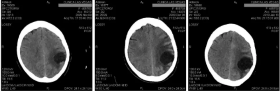
Our real data comes from a set of images of a brain tumor from the same patient, taken with Computer Tomography (CT) at intervals of one month between each of them, as can be seen in Figure 1.
Figure 1 – Original CT images at intervals of one month
This particular tumor is found in the Central Nervous System and is called glioblastoma multiform. In conformity with the World Health Organization, this tumor is the more aggressive tumor and the type and grade is according to IV-th classification. In IV-these images we can note a presence of multiple tumors in the body, indicating metastasis. These metastatic tumors are children of primary
tumors that can come from the breast, lung, colon, stomach or skin (melanoma); in our case in Figure 1, the original one comes from brain tumor.
A patient with glioblastoma multiform has an average life span of one year, receiving radiation therapy, steroids, anticonvulsants. Otherwise the patient dies long before one year. For the patients affected by this type of tumor, it is noted neurological deterioration producing difficulty in organizing ideas and their expres-sion in a coherent way. Then they lose the mobility function as the tumor affects the brain and areas dedicated to memory, speech, motor function, etc. This is the reason why there are few images that can be used for each patient, usually one or two. It is quite rare when the patient survives to make the third CT, however this is the case for our patient.
From this complete set of analysis we selected three images taken in the same plane: one from November 9th of 2009, one from December 8th of 2009, and the last from January 10th of 2010. We use the first two images to model the growth, and then we perform a prediction on the third temporal instant to compare with the existing original image.
The very first step is to perform a preliminary data processing for registration of the coordinates of all the images and normalization of the intensity range of the provided images. For patient identity protection, we first cleaned all personal data contained in the CT images. We need to make sure that all three images have the same cartesian coordinates, and that the tumor is located on the same grid points.
For image registration we used labeled landmark. The reference point in this case is the center of the brain and/or fixed points of the skull. We overlapped the images and applied transformations based on translations, rotations and in some cases affine transformations so that the three images perfectly match. After determination of the boundary of each tumor, in the case that the infected cells from each month are not overlapped, we make a second registration using the same technique and taking into account the curvature points of each boundary.
Once all the three images have a good overlap, we proceed to normalize the images. The normalization process scales the brightness values of the image so that the darkest point becomes black and the brightest point becomes as bright as possible, without altering the contained information. In other words, the normal-ization process fits the intensity values of the pixels within the range [0, 255]. A value of 0 represents black and 255 refers to white. This normalization procedure is necessary to be sure that the intensity color of one particular pixel from the first image is directly comparable with the intensity color of the same pixel from the second and third images. It is also important that the same pixel has the same cartesian coordinates in all images (guaranteed by the registration procedure).
Once we have all the images registered and normalized we can proceed to locate the tumor and extract the pixel information. In order to better locate the cancer tumor we use the image histogram, also named intensity histogram. Once located the site of the cancer tumor, we then go on to define the Region Of Interest (ROI). The ROI must include the boundary of the cancer tumor. Each point of the ROI (i.e., each pixel of the image) can be treated as events of a point pattern with a mark given by the intensity level color, which denotes if that event belongs to the
cancerous tissue or not.
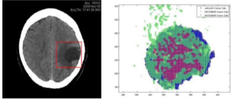
Figure 2 – ROI in the registered images (left) and infected cells (right)
To not overload the computer performing unnecessary calculations, we must define the ROI just enough to contain the studied tumor and the additional tissue, but not to small to not lose the influence of marginal likelihood. The user can define the ROI in different forms (square, rectangle, circle, etc.) that better fit the used method.
In Figure 2 we show the processed image and the ROI defined as a square. In the right side we plot the infected points from all three images within the ROI (red for November, green for December and blue for January).
2.2. Simulated data
Due the fact that few patients survive long enough to make a third analysis, and because the European Union has adopted a set of rules and laws to protect the patients and personal information, there are not such database with open access. Under the EU law, personal data can only be gathered legally under strict conditions. Also, any persons or organisations who collect and manage personal information from patients must protect it from misuse and must respect certain rights of the data owners which are guaranteed by the EU law. Taking into account these facts and due the necessity of more input data, we proceeded to implement a Matlab function to simulate such input data, i.e. closed random curves.
The simulated data consists of sets of closed curves with different number of contour points spread in a round area (see Figure 4). Each set contains three discrete closed curves with different radius, keeping the same center. Curves are created by joining a predetermined number of points arranged in a circle of radius defined by the user plus a uniformly distributed random variable. Each curve is simulated with a different number of contour points.
3. Prediction and descriptive methods
3.1. Bayesian spatio-temporal prediction
Markov Chain Monte Carlo (MCMC) combined with the Stochastic Partial Dif-ferential Equation (SPDE) approach were the motivation for the INLA package
within the R software. The library was initiated by Rue and Martino (2006) and subsequently improved through contributions of Rue et al. (2007), Rue et al. (2009), Lindgren et al. (2011), and Lindgren and Rue (2015). This INLA package is generally used to design stationary and non-stationary spatial models, spatio-temporal models, and log-Gaussian Cox point process models.
The data set extracted and used for modeling tasks consists of three matrices
P1, P2and P3(one from each image) with dimension (n× m), where n represents the number of pixels from the ROI, and m are the covariables. In our case the ROI has 130× 130 pixels, as can be seen in the right hand side of Figure 2, and thus the number of lines for each matrix P1, P2, P3 is 16900. The columns of the matrices P1, P2, P3contain the following data: (a) column 1: x-coordinate of each pixel; (b) column 2: y-coordinate of the pixel; (c) column 3: intensity level in a grey scale (the values are between [0, 255]); (d) column 4: distance from center of the tumor to the pixel; (e) column 5: logical variable: 1 if the pixel is an infected cell, and 0 otherwise.
Note that the i−th pixel has coordinates (xi, yi) in the plane, and if we denote by s = (s1, ..., sn) the set of all 16900 pixels, we do have a collection of observations evaluated at the pixels s at each temporal instant t, for a set of temporal moments (t1, ..., tn).
Spatio-temporal data can be idealized as realizations of a stochastic process Z indexed by a spatial and a temporal dimension
Z (s, t)≡{z(s, t)|(s, t) ∈ D × T ∈ R2× R} (1) where D is a (fixed) subset ofR2 and T is a temporal subset ofR.
We consider a model with response variable the pixel intensity, and based on Figure 2 the physicians consider that an intensity between 38 and 60 is a direct indicative of an infected pixel. Considering si the corresponding pixel, let
ηit= ηt(si) be the value of its intensity at time t. Following Vlad et al. (2015a), this response variable is a Poisson distributed counting variable and we specify the log-intensity of the Poisson process by an additive linear predictor (Illian et al. (2012)) as follows ηit= β0+ M ∑ m=1 βmXitm+ L ∑ l=1 fl(vli) (2)
where β0i is a scalar which represents the intercept, β = (β1, .., βM) are the co-efficients which quantify the effect of some covariates X = (X1, .., XM) on the response, and f = {f1(.) , .., fL(.)} is a collection of functions defined in terms of another set of covariates. By varying the form of the functions fl(.) we can estimate different kind of models, from standard and hierarchical regression, to spatial and spatio-temporal models (Rue et al. (2009)). Given the specification in (2), the vector of parameters is represented by θ ={β0, β, f}.
We note that we could argue why the gray-scale value should be considered as a count. Following standard practice in this context (see Qi et al., 1993; Epifanio
et al., 2011; Vlad et al., 2015a), a pixel (in our case the ROI has 130× 130 pixels)
a particular cell area. For each subpixel, we can define a Bernoulli random vari-able taking the value of 1 if the intensity level ranges between 38 and 60. The sum of these random variables defines a Binomial one for the corresponding pixel providing information on the infection of that pixel. In addition, the Binomial distribution is approximated by a Poisson random variable (see Epifanio et al., 2011; Vlad et al., 2015a). There is a one-to-one correspondence between the value of this distribution and the intensity (gray-scale) value.
Thus the intensity value, given by a discrete integer random variable, can indeed be considered as a proxy for the number of infected (sub)pixels per cell area. It is also true that the assumption of Gaussianity should be reasonable considering the range of the values. In this case, there is a large literature on Gaussian random fields for large data with exact inference (see Rue and Held, 2005). In any case, in this paper we have followed standard practice in this image-based context by assuming a count distribution, but of course the Gaussian approximation could be worth exploring.
Following the results in Vlad et al. (2015a), we consider the particular spatio-temporal additive model
ηit= β0+ β1Xit+ Si+ τt+ υit (3) where β0 is an overall constant that levels the risk, β1 represents the coefficient that quantifies the effect of the distance in the response, Xitis the distance from the center of mass to each infected pixel at time t, Siis a spatial random effect that accounts for the spatial dependence and represents the heterogeneity accounting for the variation in relative risk across different infected cells, τtis a temporal ran-dom effect accounting for the temporal dependence, and υit is a spatio-temporal random effect in relation to the spatio-temporal interaction. A spatio-temporal correlation structure is a complicated mathematical entity and its practical esti-mation is very difficult. We thus assume separability in the sense that we model separately the spatial correlation by the Mat´ern spatial covariance function, and the temporal correlation. Following Vlad et al. (2015a), both the temporal de-pendence (on t) and the spatio-temporal interaction (on i and t) are assumed to be smoothed functions, in particular Random Walks of order 1 (RW1). This is a pragmatic assumption that is often considered when working with cancer growth, and motivated by the behavior of cancer growth that generally suggests this type or dependence on the previous temporal instant.
We used the conjugate prior to the Poisson likelihood, which is a Gamma dis-tribution function. Indeed, with the aim of checking the robustness of our method-ological choice we used several other (non-conjugate) priors for the precision pa-rameters (in particular Gaussian and at priors), and the posterior distribution for the precision hyper-parameters did not changed significantly. Thus we included the Gamma conjugate priors used generally in INLA. The priors were specified on the log of the unstructured and the structured effect precision. The fitted model was checked using the Deviance Information Criterion (DIC) (Spiegelhalter et al., 2002), which is a Bayesian model comparison criterion, and the conditional predic-tive ordinate (CPO) (Pettit, 1990; Geisser, 1993). Our model showed reasonable low CPO and DIC values. We also calculated the correlation coefficient between
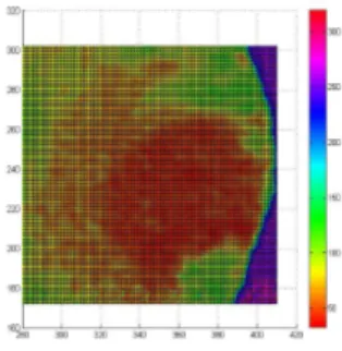
the predicted and observed values, and the root mean square error (RMSE). De-tailed analysis are shown in Vlad et al. (2015a). Figure 3 shows the corresponding prediction map using the fitted model defined in (3), highlighting the regions where the cancer has a higher probability of extending in some future time.
Figure 3 – Prediction map using a Bayesian approach
3.2. Geometrical methods
We now focus on the geometrical approach proposed by Vlad et al. (2015b). We just consider the boundary of the tumor at different times, not the entire tissue, and we assume that the speed of variation in time (the growth speed) is constant in each direction (but not equal).
We first calculate the exact coordinates of moving points through solving the corresponding movement equations. Denote by x(t) and y(t) these coordinates at time t.
For a growing object in the plane, the state at time t is a random subset Ytof Z2consisting of the “infected sites”, and Y0(initial tumor) consists of a single site. It is deduced that the tumor shape Ytat present time t depends on the structure of the initial tumor shape Y0. Then the tumor shape in a future time Yt+∆t is a function which depends on the edge and structure of the cancer in the present time Yt, and also on some external factors like mitosis, nature of cancer (benign or malign), density, etc (all these factors can be included in a function g(t)). Then,
Yt+∆t= f (Yt) + g(t) (4)
The boundary of the tumor at different times is represented by a closed curve, and to predict the tumor growth we need to find the curve αt+∆t based on obser-vations at times ti < t+∆t. We now comment on two methods based on geometric properties of curves and vectors, the main differences between them consisting of the different directions of the vectors chosen at points Pi∈ αt(si).
3.2.1. The radius method
In this case we consider star-shaped domains from an origin O(x0, y0), and corre-sponding vectors represented by the radius line from this origin to each point Pt1
of the first curve α1 in that direction.
This method is quite simple to understand from the theoretical viewpoint and also from the point of view of calculus. Starting from the center point of the original tumor O = O(x0, y0), we construct a line from each contour point Pt1
i of the curve α1 and continue to the intersection of the second contour α2, which gives the points of the second contour Pt2
i , for each i = 1, 2, . . . , n, where n is the number of contour points (see Figure 4a). These lines with the direction from the center point O to the points Pt1
i will be called radius vectors. The estimated points of the second curve αt1+∆tare denoted by P
t2 1 , P t2 2 , . . . , P t2 n . The third curve (the simulated curve) is αt1+2∆t because the time intervals
be-tween t1, t2 and t3 are supposed to be equal. These three curves are denoted by
α1, α2 and α3 respectively.
For each i = 1, 2, . . . , n the distances between Pt1
i and P t2
i are the values of the function f1(Pt1
i ) and we can calculate the spatial coordinate of the contour points Pt3
i at time t1+ 2∆t.
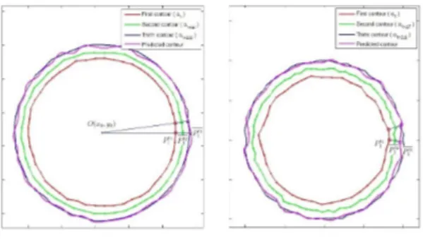
Figure 4 – Simulated tumor boundary and geometrical prediction methods: radius
method (left), normal method (right)
Following Vlad et al. (2015b), the prediction results using the radius method are precise for both non-parametric curves and irregular parametrical curves (see Figure 4). See subsection 3.2.3 and Figure 5 for practical results.
3.2.2. The normal method
The normal method of predicting growth is a particular case of curve evolution, where each point of a curve α moves in the normal direction with speed equal to the function f (s) at that point. Consider a family of smooth closed curves α(s, t) where t means time and s is the parameter of the curve (s and t are independent) and suppose that α(s, ti) = αi(s), for i = 1, . . . , n.
The mathematical formulation in this case is
∂α(s, t)
∂t = F (s)N (s, t), i = 1, . . . n− 1, (5)
where N (s, t) is the normal vector to the curve α(s, t) and F (s, t) is the speed function. In principle the function F may depend on many factors like local and
global properties of the growing curve and time t. However, in our method F does not depend on t.
For numerical implementation we approximate
∂αi(s, t)
∂t |ti ≈
αi(s, ti+ ∆t)− αi(s, ti)
∆t = f (s)Ni(s), i = 1, . . . n− 1. (6) Then, since ∆t is constant for each i, we have
αi+1(s)≈ αi(s) + ∆tf (s)Ni(s) = αi(s) + f0(s)Ni(t). (7) Several examples of functions F (s, t) can be found in Belyaev et al. (1999), for instance, when the function is the curvature of the initial curve, we have a curvature-driven evolution of the initial curve α0.
For prediction purposes, the first vector is the normal vector−−−−−→N1(Pt1
1 ) to the surface αt in point P1(x1, y1), and in that direction we find the point Pi(xi, yi) i.e Pt2
1 at the intersection with the second contour αt+∆t. Starting from this point in the direction of the normal vector to the second contour, we calculate the spatial coordinates of the predicted point Pt3
1 (see Figure 4). The predicted tumor boundary α3(si) is plotted using B-splines between obtained points Pit3.
3.2.3. Prediction results
The usual data consists of at least two curves that bound two growing planar domains. The first curve can be the contour of one tumor when it was discovered (at time t), and the second curve is the same tumor after some temporal instant ∆t. For real data analysis both curves can be provided by two CT analysis, at a time interval.
Although these curves are continuous (parameterized) curves, all our calcu-lations, which are based on the comparison of these curves, are done on digital curves, that is, a discretized version of the parameterized curves using contour points of each curve.
The values of the vectors from a specific time can be calculated if we know the parametric function or the discretized step. From both methods of calculus the input data represent the coordinates of the contour points.
We applied both prediction methods to the input data shown in Section 2. Starting from the first two images we calculated the prediction of growth of this tumor, which we scheduled for January 10th, 2010. We can directly compare the results of the prediction methods, with the third image from the set of analysis. The results are shown in Figure 5.
We note that the precision of the prediction results is influenced by some factors. There are factors that depend on the user election (as for example the resolution of the CT images), others depend on the user decision when defining the input data (such as the number of contour points (radial resolution), the number of calculus iterations (longitudinal resolution), etc). The randomness in all the methods comes from the number of contour points which give the boundary. If the user decides to use a large number of points, than the algorithms provide more precisely results in contrast with more time-consuming computing resources.
Figure 5 – Brain tumor: real evolution versus prediction with the radius method (left),
and with the normal method (right)
3.3. FDA modelling
Most of the studies on tumor chancing show that any type of developing tumour has most of its proliferation constrained to the border. We thus aim at studying what affects a set of measured contours into different steps of observation by a functional data analysis approach.
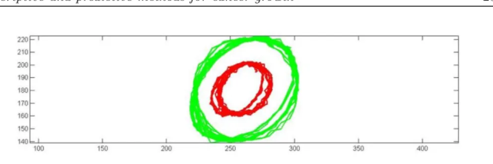
In particular as in (Romano et al. (2014a)) we propose to monitor and de-scribe the dynamics of a sequence of two sets of tumour contour functions related to two stages by using Principal Differential Analysis (Ramsay and Silverman (2005)). PDA is a technique that enables to estimate a differential operator from a functional dataset. A differential equation describes a process with changing dynamics by specifying relationships among the function and its derivatives. The scope of PDA, in this paper, is to extract the leading components of the contours in the two stages, thus it is applied on two different set of curves obtained from the tumor contours. Then a distance among the coefficients of the differential equation models is proposed to define the degree of the contour function changes. Let J be a set of individuals on which we monitor the brain tumor boundary evolution in two different steps of observation. Tumour contours are extracted by an automatic procedure for tumor image segmentation. Every point of the contour defined by the ROI is treated as a point pattern with a mark given by the intensity colors. Brain tumor outlines can be seen as a sampled closed contour of a figure in an Euclidean space. Every point psof the contours can thus be located with coordinates (Xij, Yij), i = 1, . . . , n in a first visit and (Xij∗, Yij∗), i = 1, . . . , n in a second visit. The set of contours can be identified by a set of closed curves, as depicted in Figure 6.
As in shape analysis (Epifanio et al (2011)), where functions are frequently used to represent shape several problems arise when comparing contour functions: the points are not the same from an observation to another; the starting-points are not the same from an observation to another; the senses of rotation could be different. Thus in order to overcome these problems we consider that sampled functional data (Xj(s), Yj(s)), (Xj∗(s), Yj∗(s)), j = 1, ..., J can be expressed in terms of K known basis functions. We chose in particular Fourier basis. Thus
Figure 6 – Contour function
squares fitting. The fit of the basis function is not penalised since the differences among the contours depend on the curvature.
Each curve is determined by the coefficients in these basis, and each function is computable for any argument value. This has been performed by means of FDA library Ramsay and Silverman (2005). A global registration criterion for finding a shift and a rescaling shape contour step have been performed. We look for the optimal wrapping functions maximizing the similarity between the curves in both the two steps and a target curve. The mean curve of the first set of curves (the “not deformed” curves) is used as target curve for registration criterion. The estimated means are then updated by re-estimating them from the registered objects.
Moreover, in order to have the same number of points for all functions, we evaluate the functions in 100 equidistant points from 0 to 1 as in Romano et al. (2014a). For each individual j there are two pairs of functions of the space s, (Xj(s), Yj(s)), s∈ [0, 1].
Because the structure of our data is sinusoidal it seems appropriate to set out a second order differential equation model that can capture contour function dynamics.
We define the following non-homogenous differential operator for the couple of functional contours in the two steps (for simplicity we report only the ones related to the first step):
LX(s) = αx(s) + ϵx(s) (8)
LY (s) = αy(s) + ϵy(s)
where LX(s) and LY (s) are defined as
LX(s) = β1x(s)DX(s) + β2x(s)D2X(s) + D3X(s) (9)
LY (s) = β1y(s)DY (s) + β2y(s)D2Y (s) + D3Y (s)
and where the differential operator D can be written as
D3X(s) = αx(s) + β1x(s)DX(s) + β2x(s)D2X(s) (10)
The two set of contours modeled by a linear differential operator are re-spectively characterized by six functions weights coefficients: αx(s),αy(s),β1x(s),
β2x(s), β1y(s), β2y(s) for the first step and αx∗(s),αy∗(s),β1x∗(s), β2x∗(s), β1y∗(s),
β2y∗(s) for the second step, then DX(s) can be seen as the velocity contour of the
j−th patient; D2X(s) as the acceleration contour and D3X(s) is the wide margin contour of the j− th patient.
Thus αx(s) is a space-varying intercept, β1x(s) is the space-varying coeffi-cient relating velocity to the wide margin contour and β2x(s) is a space-varying coefficient relating acceleration to wide margin contour. This stands for the X coordinate, but the same applies for the Y coordinate.
A least square criterion is used for estimating these functions, in particular a 34 B-Spline basis functions of order 6 is used to estimate the functional form. Once estimated the PDA model of the first set of contours, we propose to fit the data of the second step with the first estimated model. Thus in analogy with regression we build the equation with the first data set and then predict the response for a new one related to the second step.
We pursue a somewhat different approach by introducing an Euclidean distance among the coefficients of the two models estimated into the two steps. This distance seeks to investigate the modes of variability from the first to the second step of observation.
The twelve functions obtained by estimating the Principal Differential Equa-tion give indicaEqua-tion on the dynamic variability, thus we define the following dis-tance among the two models. Let us consider two models P dA, P dA∗ defined on the same support S:
- model 1: P dA = {αx(s), αy(s), β1x(s), β2x(s), β1y(s), β2y(s)}, - model 2: P dA∗= {αx∗(s), αy∗(s), β1x∗(s), β2x∗(s), β1y∗(s), β2y∗(s)}, each of them can be defined by a compound of six functions.
The distance between P dA, P dA∗ is given by d(P dA, P dA∗) (see Romano et al. (2014a)). Since it is a simple measure, can be visualized as the square root of the sum of the squared length of the vertical lines for the six functions of the models.
In this sense it allows to quantify the diversity in terms of the main character-istics among two consecutive steps. If more than two images are available it takes the dynamic evolution of the distance among the contours.
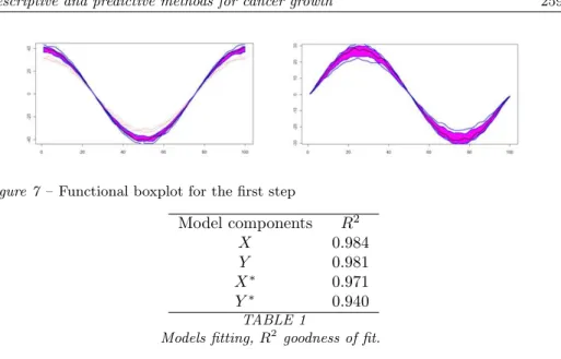
The dataset we analyse is composed of 15 brain tumor contour functions. The tomography has been done in the same conditions for both the steps of the ob-servations and for all the patients. If there was some differences the images was registered to have the same benchmarks. The procedure has removed most of the misalignments variation, making it easier to compare curves from different sub-jects. The variability captured by the optimal wrapping functions found during this alignment process is shown in Figure 7.
The boxplot highlights that there are two contour functions that seem to be anomalous, it means that they have very different shape from the other (see Fig-ure 7). There is variability, but the distribution is geometrically symmetric and compact without any significant outliers.
Figure 7 – Functional boxplot for the first step Model components R2 X 0.984 Y 0.981 X∗ 0.971 Y∗ 0.940 TABLE 1
Models fitting, R2 goodness of fit.
We apply two PDA on the two stages. Both the components in the two steps yield good fitted values. Points around 0.9 are shown in Table 1.
The estimated models in the two steps and their explained functional variabil-ity can be summarised by their coefficients. We illustrate in Figure 8 the esti-mated coefficients for the first and second step, related to the the X-component, respectively: αx(s) (top left), βx1(s) (top right) and αx∗(s) (bottom left), βx∗1(s) (bottom right). The pick of the curves shows the zones in which the contour functions increases most rapidly, which indicates that differences between the two steps may be localised to particular tract regions.
Figure 8 – Estimated coefficient functions for the X component. From top left to bottom
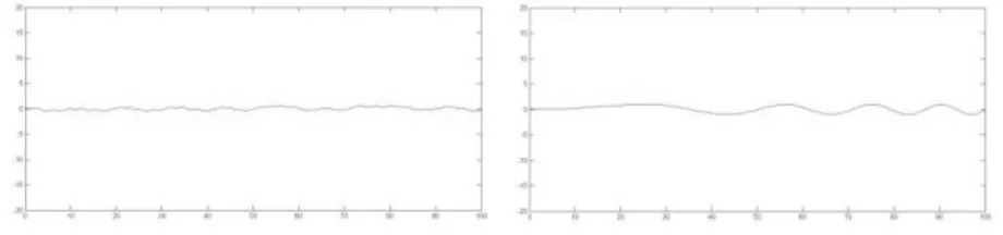
The first coefficient, for both the steps (that is the forcing functions), is roughly a mean shift indicating that the overall level of variability varies across subjects over the full domain of the contour functions. The forcing functions can be thus considered as an indicator of large source of variability rather than the coefficients
β2xand β2x∗ that have no impact on the model as can be seen in Figure 9.
Figure 9 – Estimated coefficient functions β2x(s), β2x∗(s) for the first and second step
We want to investigate the shape variation among the two steps, obtaining a distance among two fitted models. The normalised distance among the coeffi-cient is 0.6, difference due mainly to the forcing component. Despite the general similarities, there are important differences among the contour. It is likely that the first model is a reference model to monitor the variability of the shape and the velocity of the tumor contour propagation has a big weight in controlling the model changes.
4. Conclusions
The development of tumor models is important as they offer a way to better un-derstand the kinetic growth of malignant tumors which may lead to the develop-ment of successful treatdevelop-ment strategies. We have presented here a mathematical-statistical approach to analyze the spatio-temporal dynamics of brain tumors. They come in form of processed computer tomography images. We interpret them as collections of image pixels with varying degrees of color intensity levels. As such, they can be considered as a stochastic process, and we make use of spatio-temporal stochastic processes as the right statistical framework.
In addition, we set our modeling strategy within the Bayesian framework which opens doors to model spatial heterogenity, temporal dependence and spatio-temporal interactions amongst the pixels, providing a general modeling framework for such dynamics. Using this framework, we are able to predict cancer growth in space and time, and show real data analysis. The results are shown to be satisfactory for all models.
We deal with contours as continuous functions which better represent the con-tinuous form and the nature of the data analysis by the use of FDA. We have proposed to use Principal Differential Analysis as a novel application of FDA in image analysis. The space-varying coefficient function relating velocity to wide margin contour gives summaries components. Moreover a linear combination of the contour derivatives gives a prediction of the tumor contour function deforma-tion.
We have also proposed a geometrical approach and implement two simple com-putational methods to predict the tumor boundary evolution. The normal and ra-dial methods are quite simple but produce great results. The errors between real evolution and predicted evolution are more than satisfactory and may be used from physicians and patients to note if the prescribed treatment has the desired effect, and according to this, if necessary, to take the decision of surgically intervention. In a the future research we want to develop a new logical method to predict the evolution in time of tumor with more input variables like the intern structure of tumor tissue, density, tumor type and classification, patient age, sex, etc.
Acknowledgements
The present work has been partially supported by grants P1-1B2012-52, and MTM2013-43917-P from Ministry of Economy and Competitivity.
References
A. G. Belyaev, E. V. Anoshkina, S. Yoshizawa, M. Yano (1999). Polygonal
curve evolutions for planar shape modeling and analysis. International Journal
of Shape Modeling 5: 195-217.
M. Bramson, D. Griffeath (1981). On the Williams-Bjerknes tumour growth
model. The Annals of Probability 9: 173-185.
N. Cressie (1991) Modelling growth with random sets. Spatial Statistics and Imaging, A. Possolo and C.A. Hayward, eds, IMS Lecture Notes Monogr. Ser.
20. IMS, Hayward, CA.
I. Epifanio, N. Ventura-Campos (2011) Functional data analysis in shape
analysis. Journal Computational Statistics and Data Analysis 55: 2758-2773.
J. B. Illian, S. H. Sorbye, H. Rue (2012). A toolbox for fitting complex spatial
point processes models using integreted nested Laplace approximations (INLA).
The Annals of Applied Statistics 6: 1499-1530. INLA (2012) R-INLA project, 2012.
A. R. Kansal, S. Torquato, G. R. Harsh, E. A. Chiocca, T. S. Deisboeck (2000).
Simulated brain tumor growth dynamics using a three-dimensional cellular au-tomaton. J. Theor. Biol 203: 367-382.
T. Lee, R. Cowan (1994). A stochastic tessellation of digital space. In Math-ematical Morphology and Its Applications to Image Processing (J. Serra, ed.) 217-224. Dordrecht: Kluwer.
F. Lindgren, H. Rue, J. Lindstrom (2011). An explicit link between Gaussian
fields and Gaussian Markov random fields: The SPDE approach (with discus-sion). Journal of the Royal Statistical Society, Series B 73: 423-498.
F. Lindgren, H. Rue (2015). Bayesian spatial modelling with R-INLA. Journal of Statistical Software 63.
MATLAB (2014). Image processing toolbox. Matlab user guide. Available at URL
www.mathworks.co.uk/help/pdf doc/images/images tb.pdf .
A. S. Qi, X. Zheng, C. Y. Du, B. S. An (1993). A cellular automaton model
of cancerous growth. Journal of Theoretical Biology 161: 1-12.
J. O. Ramsay, B. W. Silverman (2005). Functional Data Analysis. Second Edition, Springer-Verlag, NY.
E. Romano, I. T. Vlad, J. Mateu (2012). Automatic Contour Detection and
Functional Prediction of Brain Tumour Boundary. Analysis and Modeling of
Complex Data in Behavioural and Social Sciences. PADOVA: CLEUP, ISBN: 978-88-6129-916-0, Anacapri, Italy, 3-4 Settembre 2012.
E. Romano, J. Mateu, I. T. Vlad (2014a) Principal differential analysis for
modeling dynamic contour evolution. A distance-based approach for the analysis of Gioblastoma Multiform. Submitted.
E. Romano, J. Mateu, I. T. Vlad (2014b).A functional predictive model for
monitoring variation in shapes of brain tumours. Technical Report.
H. Rue, L. Held (2005) Gaussian Markov Random Fields. Theory and
Applica-tions. Chapman & Hall/CRC: Boca Raton.
H. Rue, S. Martino (2006) Approximate Bayesian inference for hierarchical
Gaussian Markov random fields models. Journal of Statistical Planning and
Inference 137: 3177-3192.
H. Rue, S. Martino, N. Chopin (2007). Approximate bayesian inference for
latent gaussian models using integrated nested laplace approximations. Statistics
Report No. 1, Department of Mathematical Sciences, Norwegian University of Science and Technology, Trondheim, Norway.
H. Rue, S. Martino, N. Chopin (2009). Approximate Bayesian Inference for
Latent Gaussian Models using Integrated Nested Laplace Approximations (with discussion). Journal of the Royal Statistical Society B 71: 319-392.
I. T. Vlad, P. Juan, J. Mateu (2015a) Bayesian spatio-temporal prediction of
cancer dynamics. Computers and Mathematics with Applications 70: 857-868.
I. T. Vlad, J. Mateu (2015) A geometric approach to cancer growth
pre-diction based on Cox processes. Journal of Statistics: Advances in Theory and
Applications 13: 1-32.
I. T. Vlad, J. Mateu, X. Gual-Arnau (2015b). Two handy geometric
Summary
Cancer is a widely spread disease that affects a large proportion of the human popula-tion, and many research teams are developing algorithms to help medics to understand this disease. In particular, tumor growth has been studied from different viewpoints and several mathematical models have been proposed. In this paper, we review a set of com-prehensive and modern tools that are useful for prediction of cancer growth in space and time. We comment on three alternative approaches. We first consider spatio-temporal stochastic processes within a Bayesian framework to model spatial heterogeneity, tempo-ral dependence and spatio-tempotempo-ral interactions amongst the pixels, providing a genetempo-ral modeling framework for such dynamics. We then consider predictions based on geo-metric properties of plane curves and vectors, and propose two methods of geogeo-metric prediction. Finally we focus on functional data analysis to statistically compare tumor contour evolutions. We also analyze real data on brain tumor.