11. INTRODUCTION
The concern in the high levels of population density had its boom during the 60’s and 70’s. Obviously, the idea was to study not only its causes but also its effects. Indeed, as Baldassare (1978) proved, a large number of factors led to believe to a substantial part of the scientific community and most of the general population that a high level of density, in terms of people, has serious detrimental effects on humans. The majority of these studies focused on the effects of high levels of people density on human behavior. From these studies, it was clear that it was necessary to distinguish between density at the level of macro-environment (people per hectare, for example) and crowding in the micro-environment, such as crowding in home (Carnahan et al., 1974; Galle and Gove, 1978).
Recently, it seems like the interest in the high levels of density of people has come back. For example Marx and Stoker (2013), referring to slums, which are informal
settlements in and around cities in the developing countries, estimates that 450 million new housing units would be needed in the next 20 years just for accommodating households in urgent need of housing due to the increase of migrants to the existing slum populations. Said so, it is clear that there is a strong correlation between poverty and high density of people in the house. Indeed, one of the most used methodologies for measuring poverty, especially in Latin America, the Unsatisfied Basic Needs (UBNS) method uses as an indicator for determining a poverty situation the fact that there are more than three people per room in the house.
In this paper, authors focus on the household crowding. According to Lawton (1961), household crowding is a difficult concept to express since acceptable standards of intensity of household occupancy vary from time to time, from place to place and as between social classes. Moreover, indices of crowding can be selected from a variety of census data, including the number of people, the number of rooms, the number of households and the number of dwellings of various sizes. The most extended index for approaching to household crowding is the people per room measure: a
An approximation to Household Overcrowding:
Evidence from Ecuador
Díaz Juan Pablo1; Romaní Javier2
1Escuela Politécnica Nacional, Facultad de Ciencias, Quito, Ecuador 2 Universidad de Barcelona, Facultad de Economía y Empresa, Barcelona, España
Abstract: This paper addresses the household overcrowding problem. To do so, a binary choice model with logit specification is constructed. The cross section data used in the empirical analysis comes from Ecuador which is a developing South American country. Although, household overcrowding has more incidence in developing countries, it also takes place in developed economies. The findings of the research suggest that a set of variables related to the head of the household like his/her gender, age, and level of education affect the probability of being under overcrowding situation in the household. Furthermore, the regime of tenancy under which the household is living in the dwelling also influences the probability of being in overcrowding situation.
Key words: Ecuador, household overcrowding, crowding, logit modelling.
Una aproximación al Hacinamiento de Hogares:
Evidencia del Ecuador
Resumen: En este trabajo se aborda el problema de hacinamiento de los hogares. Para ello, un modelo de elección binaria con especificación logit es construido. Los datos de corte transversal utilizadas en el análisis empírico proviene de Ecuador, que es un país en desarrollo de América del Sur. Aunque, el hacinamiento de los hogares tiene más incidencia en los países en desarrollo, también tiene lugar en las economías desarrolladas. Los resultados de la investigación sugieren que un conjunto de variables relacionadas con el jefe de la familia como su sexo, edad y nivel de educación afecta a la probabilidad de estar en situación de hacinamiento en el hogar. Por otra parte, el régimen de tenencia en las que la familia está viviendo en la vivienda también influye en la probabilidad de estar en situación de hacinamiento.
household is considered in a crowding situation if there are more than three people per bedroom; however, this index presents limitations as a measure of intense of occupancy since it does not take into account the size of the household (for example, a household formed by 10 people and 5 rooms is not ¨crowded,¨ meanwhile a household formed by 3 people and 1 room is) neither their particular needs which lead to a collective generalization. Despite these inconveniences, this measure of crowding gives us an idea about the particularities of the household and the society.
This paper is composed as follows; first, it is presented a review of the literature about the household crowding. Secondly, the methodology that is used in the empirical analysis is presented, basically binary choice models. Then, it is shown an empirical analysis using cross section data about the probability of being in a household crowding situation. The condition that tells us if a household is in a crowding situation is if there are more than three people per bedroom in the household. The data is from Ecuador which is a developing country located in the North West part of South America. After that, it is discussed the results obtained in the estimates. Finally, some conclusions are presented.
2. LITERATURE REVIEW
In general terms, there are several factors that contribute to the household crowding. First, there is the demographic factor which is basically represented by the vegetative population growth rate and migrations. Second, the physical factors of the dwelling and its environment. Finally, the social factor also plays an important role. As physical factors of the house one can point out the design of the dwelling, the habitability of the construction, the sanitary situation, conditions of the settlement place and the physical channels of social integration like roads, nearly schools and so on. The social factor refers to the housing density and tenancy regime. The housing density is the relationship between the number of people and the available space. As a matter of fact, the housing density becomes crowding when this relationship between people and available space exceeds a tolerable limit. On the other hand, the tenancy regime is related to the condition of ownership for the people living in a certain house like owner, renter, usurper or borrower (Puga, 1983). It is important to mention that there are several approaches to measure crowding. For example, people per bed, people per bedroom, families per dwelling, and dwellings per piece of land (Iglesias de Usel, 1993). Another indicator for measuring the intensive usage of the space is the quantity of square meters per person. It is important to say this because authors want to point out that there is not a unique form to define crowding. Indeed, the threshold from which it can be considered an intensive usage of the space varies according to the level of development of societies, cultural and historical realities.
The theoretical literature on the consequences of crowding on individuals basically focuses on physical and psychological repercussions. About the physical effects, crowding could be a determinant factor for illness propagation not only in developing countries, but also in the developed ones. For
instance, Baker et al. (2008) proved that Tuberculosis incidence in New Zealand is associated with household crowding. Moreover, an alarming fact about the crowding is that it especially affects children in their growing-up and development processes. Furthermore, according to Iglesias de Usel (1993) and Puga (1983) there are causal relationships between crowding and low test score performing and high juvenile crime rate.
Regarding the psychological effects researchers have determined two main alterations in crowding situations: lack of privacy and easiness of circulation (Lentini, 1997). Regarding the privacy, it is clear that it is a required good for a person, for couples (father-mother), for gender separation, for the family as an independent social unity and for certain family activities such as sleeping, studying, etc. About the easiness of circulation, it allows the normal fulfillment of the family functions by avoiding the interferences to the freedom of circulation or the unexpected intrusions. The lack of both, privacy and easiness of circulation, creates an environment in which the members of the household may be exposed to higher levels of psychological stress than those who are not living under this condition.
Until now, it has been said that there are at least two main dimensions that help us to understand crowding in households: number of individuals in the household and the dwelling itself. Regarding the number of individuals compounding a household, there are a great number of published papers that contributes to understand the size of the household. For example, Bongaarts (2001) published a study that uses data from household surveys in 43 developing countries to describe the main dimensions of household size and their composition in the developing world. He found that the average household size varies only modestly among regions, ranging from 5.6 in the Near East/North Africa to 4.8 in Latin America. These averages are similar to levels observed in the second half of the nineteenth century in Europe and North America. Moreover, he observed that about four out of five members of the household are part of the nuclear family of the head of the household. In addition, Bongaarts suggests that household size is found to be positively associated with the level of fertility and the mean age at marriage, and inversely associated with the level of marital disruption. An analysis of trends and differentials in household size suggests that convergence to smaller and predominantly nuclear households is proceeding slowly in contemporary developing countries.
Regarding the associated effects of the size of the household, Lanjouw and Ravallion (1995) point out that there is considerable evidence of a strong negative correlation between household size and consumption (or income) per person in developing countries. It is often concluded that people living in larger and (generally) younger households are typically poorer. There has been much debate on which is the 'cause' and which is the 'effect' in this correlation. The position one takes in this debate can have implications for policy, including the role of population policy in development, and the scope for fighting poverty using demographically contingent transfers. In addition, they
suggest that the existence of size economies in household consumption cautions against concluding that larger families tend to be poorer. The poor tend to devote a high share of their budget to rival goods such as food. But certain goods (water taps, cooking utensils, firewood, clothing, and housing) do allow possibilities for sharing or bulk purchase such that the cost per person of a given standard of living is lower when individuals live together than apart.
About the variables explaining the size of the households, one can found studies that use, for example, demographic variables. That is the case of Burch (1970) who investigates the influence of demographic variables (viz., mortality, fertility, age at marriage) on average household size under different family systems-nuclear, extended and stem. His study suggests that under all family systems, average household size is positively correlated with fertility, life expectancy, and average age at marriage. Households under nuclear and stem family systems never exceed 10 persons on average. By contrast, under extended family systems, when mortality is low and fertility is high, average household size reaches levels seldom if ever observed in reality, e.g., 25 persons per household. Large households under the extended family system also tend to be fairly complex, often containing 5 or more adults. A number of modifications in the model would make for greater fit between model and real family systems. A more fruitful approach would involve the simulation of household formation and development.
With respect to the types or forms of household crowding, as it has been said above, there is not a unique unit of measure for it. However, the most extended measure is the people per room. Despite of its limitations, which are basically not considering the size of the household neither their specific needs, it is helpful to draw an aggregate picture of the phenomenon. In that sense, Lentini (1997) categorizes as semi-critical crowding when there are more than two people per bedroom and as critical crowding when there are more than three people per bedroom.
3. METHODOLOGY
Authors will use the framework of the binary choice models for our empirical analysis. According to Verbeek (2004), binary choice models (or univariate dichotomous models) are designed to model the ‘choice’ between two discrete alternatives. These models essentially describe the probability that yi = 1directly. In general, Equation (1):
𝑃{𝑣𝑖= 1⎸𝑥𝑖} = 𝐺(𝑥𝑖, 𝛽) (1)
for some function G(.). This equation says that the probability of having yi = 1 depends on the vector xi
containing individual characteristics. So, just for giving an example, the probability that a household is in a crowding situation depends on its income, head-of-the-house education level, age and marital status. Clearly, the function G(.) should take values in the interval [0, 1] only. Usually, one restricts attention to functions of the form G(xi,β) = F(x´iβ). As F(.)
also has to be between 0 and 1, it seems natural to choose F
to be some distribution function. Common choices are the standard normal distribution function, Equation (2):
𝐹(𝑤) = φ(w) = ∫ 1 √2π w −∞ exp {− 1 2t 2} dt (2)
Leading to the probit model, and the standard logistic distribution function, given by Equation (3):
𝐹(𝑤) = 𝐿(𝑤) =
𝑒𝑤1+𝑒𝑤
(3)
Which results in the logit model. There is also a third option besides the probit and logit models, the linear probability model; however, the logit and probit are more common in applied work.
Both, a standard normal and a standard logistic random variable have an expectation of zero, while the linear probability has a variance of π2/3 instead of 1. These two distribution functions are very similar if one corrects for this difference in scaling; the logistic distribution has slightly heavier tails. Indeed, the probit and logit models typically yield very similar results in empirical work. Moreover, apart from their signs, the coefficients in these binary choice models are not easy to interpret directly.
Regarding the estimation and always according to Verbeek (2004), in general, the likelihood contribution of observation i with yi= 1 is given by P{yi= 1|xi} as a function of the
unknown parameter vector β, and similarly for yi= 0. The
likelihood function for the entire sample is thus given by Equation (4):
𝐿(𝛽) = ∏𝑁𝑖=1𝑃{𝑦𝑖= 1|𝑥𝑖; 𝛽}𝑦𝑖𝑃{𝑦𝑖= 0|𝑥𝑖; 𝛽}1−𝑦𝑖 (4) Where β is included in the Equations for the probabilities to stress that the likelihood function is a function of β. It is preferred to work with the loglikelihood function. Substituting P{yi= 1|xi ; β} = F(x´iβ), as seen Equation (5):
log 𝐿(𝛽) = ∑𝑖=1𝑁 𝑦𝑖log 𝐹(𝑥𝑖′𝛽) + ∑𝑁𝑖=1(1 − 𝑦𝑖) log(1 − 𝐹(𝑥𝑖′𝛽)) (5)
Substituting the appropriate form for F gives an Equation that can be maximized with respect to β. As previously said, the values of β and their interpretation depend upon the distribution function that is chosen.
Consequently, let`s consider the first order conditions of the maximum likelihood problem. Differentiating the previous equation with respect to β yields, Equation (6):
𝛿𝑙𝑜𝑔 𝐿(𝛽) 𝛿𝛽 = ∑ [ 𝑦𝑖−𝐹(𝑥𝑖′𝛽) 𝐹(𝑥𝑖′𝛽)(1−𝐹(𝑥𝑖′𝛽))𝑓(𝑥𝑖 ′𝛽)] 𝑥 𝑖= 0 𝑁 𝑖=1 (6)
Where f = F´ is the derivative of the distribution function (so f is the density function).The term in square brackets is often referred to as the generalized residual of the model. It equals f(x’iβ)/F(x’iβ) for the positive observations (yi= 1) and
-f(x’iβ)/(1 − F(x’iβ)) for the zero observations (yi= 0). The
first order conditions thus say that each explanatory variable should be orthogonal to the generalized residual (over the whole sample). This is comparable to the OLS first order conditions which state that the least squares residuals are orthogonal to each variable in xi.
For the logit model, one can simplify the Equation in (7) to
𝛿𝑙𝑜𝑔 𝐿(𝛽) 𝛿𝛽 = ∑ [𝑦𝑖− exp (𝑥𝑖′𝛽) 1+exp (𝑥𝑖′𝛽)] 𝑥𝑖= 0 𝑁 𝑖=1 (7)
Furthermore, for the probit model
𝛿ln {𝐿(𝛽)} 𝛿𝛽 = ∑ −𝜑𝑖 1−𝛷𝑖𝑥𝑖 𝑦𝑖=0 + ∑ 𝜑𝑖 𝛷𝑖𝑥𝑖 𝑦𝑖=1
=
∑𝑦𝑖=0𝜆
0𝑖𝑥
𝑖+
∑𝑦𝑖=1𝜆
1𝑖𝑥
𝑖=
∑ ( 𝑞𝑖𝜑(𝑞𝑖𝑥𝑖′𝛽) 𝛷(𝑞𝑖𝑥𝑖′𝛽)) 𝑛 𝑖=1𝑥
𝑖=
∑𝑛𝑖=1𝜆
𝑖𝑥
𝑖= 0;
(8)
With qi=2yi – 1. The solution of the Equation in (8) is the
maximum likelihood estimator 𝛽̂. From this estimate, it is possible to estimate the probability that yi= 1 for a given xi as
seen Equation (9):
𝑝̂ =𝑖
exp (𝑥𝑖′𝛽)
1+exp (𝑥𝑖′𝛽); 𝑖 = 1 … 𝑛 (9) Consequently, the first order conditions for the logit model imply that, Equation (10):
∑𝑁𝑖=1𝑝̂𝑖𝑥𝑖= ∑𝑁𝑖=1𝑦𝑖𝑥𝑖 (10)
Thus, if xi contains a constant term (and there is no reason
why it should not), then the sum of the estimated probabilities is equal to ∑iyi or the number of observations in
the sample for which yi= 1. In other words, the predicted frequency is equal to the actual frequency. Similarly, if xi
includes a dummy variable, say 1 for females, 0 for males, then the predicted frequency will be equal to the actual frequency for each gender group. Although a similar result does not hold exactly for the probit model, it does hold approximately by virtue of the similarity of the logit and probit model.
Taking into account that in the empirical work both, logit and probit specifications yields similar results, in this paper, authors will use the logit specification; however, this does not mean that the probit specification does not present also good estimations.
Data and variables. Data from the Survey of Conditions of Life (Encuesta de Condiciones de Vida) from Ecuador (INEC, 2006) is used that provides information of 13.536 households in Ecuador for our empirical analysis. The objectives of this survey were to measure the impact of the macroeconomic adjust policies and the social compensation on the households, to create monetary and non-monetary measures about the welfare distribution and the level of poorness of the households, to generate an actualized base line and useful to measure the accomplishment of the
Millennium Development Goals and Objectives, and to simplify the formulation
of
public policies that tend to reduce the levels of poorness of the population.Authors will use the information of the fifth round of the survey which collected the information between November 2005 and October 2006. Considering the 13.536 households that provided information, 8.028 of them are located in an urban area which represents the 59% of the sample; meanwhile, the remaining 5.508 households were from rural areas which represent the 41% of the sample. In addition, the information was collected from 1128 census sectors in where 12 households per sector supplied information (12 x 1128 = 13.536). It covers all the provinces of the Ecuadorean continental territory.
It is important to mention that this survey is a post-dollarization instrument. Briefly speaking, Ecuador had a severe economic crisis in 1998 that led to an emigration wave that, according estimations, caused millions of Ecuadoreans to leave their country. As a policy of stabilization, dollarization of the economy was implemented in 2000, which brought a stable economic scenario (Acosta, 2012).
Once the methodology and the data source have been defined, it is time to define the condition under which a household can be considered overcrowded or not for our empirical analysis. According to CEPAL (2001) (Comisión Económica para América Latina y el Caribe) and several other authors like Lentini (1997), authors will characterize overcrowding as it is done in most extended and accepted measure, meaning that a household will be overcrowded if there are more than three people per bedroom.
On the other hand, a household will not be crowded if this condition is not fulfilled. Since the condition is reflected in the output variable yi of the binary logit model, it will take
the value of 1 if the overcrowding condition is fulfilled (in other words, if the household is crowded, then yi=1);
otherwise, the dependent variable takes the value of 0 if the crowding condition is not fulfilled (yi=0). By doing so, it is
obtained that the 58.1% of the sample (7897 observations) fulfill the overcrowding condition and the 41.9% do not (5684 observations).
Considering the information available in the data base and the literature reviewed, it is included in the model specification several explanatory variables that are supported in previous researches. In that sense, a set of independent variables that collects information of the head of the household is included. The idea behind these inclusions is to characterize the person who runs the household and, if it is possible, suggest public policies that contribute to overcome the overcrowding condition. Considering the head of the household as the core unit in the analysis of overcrowding is an extended practice in the applied work as it is showed in Bongaarts (2001). Furthermore, since Puga (1983) proved that the regime of tenancy of the dwelling is a vital dimension in the household overcrowding as a social factor, authors also include a variable that collects this information. Additionally, a variable that presents information of the
settlement place, which in Puga (1983) called as physical factor, is included in the estimation.
Then, the estimation of the probability that for the logit model is given by Equation (11):
𝑃𝑟𝑜𝑏(𝑌𝑖= 1) = 𝑒𝑧 1+ 𝑒𝑧 (11) where: 𝑧 = 𝛽0+ 𝛽1𝐴𝑟𝑒𝑎𝑖+ 𝛽2𝐺𝑒𝑛𝑑𝑒𝑟𝑖+ 𝛽3𝐴𝑔𝑒𝑖+ 𝛽4𝐴𝑔𝑒𝑆𝑞𝑖 +𝛽5𝐸𝑑𝑢𝑐𝑖+ 𝛽6𝐸𝑡ℎ𝑛𝑖𝑐𝑖+ 𝛽7𝐻𝐷𝐵𝑖+ 𝛽8𝑇𝑒𝑛𝑎𝑛𝑐𝑦𝑖
For i = 1… 13.536. Where Yi is the dichotomous variable explained above;
β
0is the constant term in the estimation;Area is a dummy variable for the area in which the household is located. It takes the value of 1 if the household is settled in the urban area or 0 otherwise. Fixing rural as the reference category, it is expected to get a negative sign in the estimated parameter since it is thought that a household located in the urban area has less probability of being overcrowded than a one with the same characteristics located in the country side;
Gender is another dummy variable for the gender of the head of the household. It takes the value of 1 if the head of the household is a man or 0 in the case of being a woman. Fixing as reference category being a woman, the expected sign of the estimated parameter is negative since one could think that a household in which the head of the household is a man has less probability of being overcrowded than a household in which the head of the household is a woman under similar conditions. This assumption is supported in the well documented evidence in the literature that women have less income than men by doing the same job or having the same position as De Cabo (2007) proved, so it is expected that this could influence in the reduction of probability that a man as a head of the household being in an overcrowded situation compared to a woman;
Age and AgeSq are the age and the aged squared of the head of the household. It is expected to get a positive sign in the first one and a negative sign in the estimation of these parameters. The idea behind this expectation is that as the head of the household gets older, the number of members of the household increases until a certain point in which the members start to leave the house meaning that the effect of the age on the probability of being overcrowded has an inverted u shape. On the other hand, if our expectation is wrong, that would suggest that the older the head of the household, the more the number of members in it. It would evidence that the other members of the household do not leave the house as the time passes but they bring new members to the home;
Educ is the level of education of the head of the household. It is measured in years attended to formal education. Indeed, this variable works also as a proxy of the level of income of
the head of the household since it is well documented in the literature about the strong correlation between education and income;
Ethnic is a categorical variable of the ethnic self-identification of the head of the household. It is fixed as reference category ‘indigenous,’ so the other categories (mestizo2, white, black, mulato3 and other) will be compared
to it. It is expected a negative sign in the parameters of the other categories which would suggest that the other ethnic groups have less probabilities of being in an overcrowded household than indigenous households. This expectation comes from the idea that indigenous historically have been socially segregated not only in Ecuador, but in the whole America which would result in the deterioration of their living conditions;
HDB is a dummy variable that takes the value of 1 if the head of the household receives the Bono de Desarrollo Humano (rough translation: Human Development Bonus) or 0 otherwise. The Human Development Bonus is a direct cash transfer for poor families from the government. Fixing not receiving the cash transfer as category of reference, it is expected to get a positive sign in the estimated betha meaning that those households that receive the cash transfer have more probability of being in overcrowding situation;
Tenancy is a categorical variable that describes the regime of tenancy under which the household is living there. The possible alternatives are: owned and fully paid, antichresis4,
owned and paying for it, leased, given, and received for services. By fixing as reference category the first named, it is expected a variety of signs in the estimated parameters such as a negative one in the own and paying for it option or a positive sign in the leasing option.
If it is consider as crowding situation the fact that there are more than three people per room in the household, 29.8% households out of the total at a national level are overcrowded. As a matter of fact, 26.6% and 36.0% of the households are under crowding conditions in the urban and rural areas, respectively.
Regarding the ethnic self-identification, when the head of the household self-identifies as indigenous, the 48.9% of the households in this category are under crowding conditions. This percentage is 27.9% of the total in mestizo households. Moreover, when the head of the household self-identifies as white, the 24.8% of the total of households in this category are under the crowding condition.
Finally, when the head of the household self-identifies as black, the 38.8% out of the total of households in this category are under the crowding condition. As one can see,
2 It is the ethnic identification that results of the mix between white and
indigenous.
3 It is the ethnic identification that results of the mix between white and
black.
4 It is a contractual arrangement in which the owner of the house let the
other contractual part to live in the house for paying a unique quota at the beginning of the contract lapse. Once the lapse of the contract is finished, the owner of the house gives back the entire initial quota to the “leaser.”
the shares of crowded households are especially higher in minority ethnic groups (indigenous and black).
4. RESULTS AND DISCUSSION
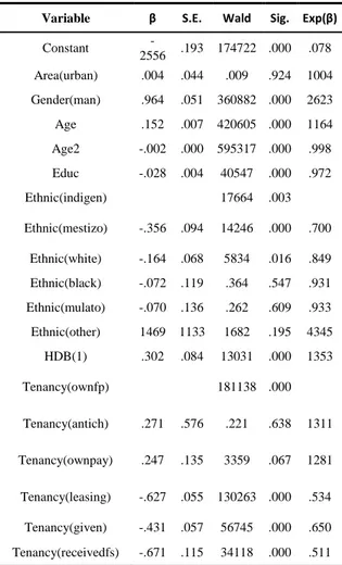
The obtained results of the binary logit estimation are as follows in Table 1.
Table 1. Results of the Model
Variable β S.E. Wald Sig. Exp(β)
Constant -2556 .193 174722 .000 .078 Area(urban) .004 .044 .009 .924 1004 Gender(man) .964 .051 360882 .000 2623 Age .152 .007 420605 .000 1164 Age2 -.002 .000 595317 .000 .998 Educ -.028 .004 40547 .000 .972 Ethnic(indigen) 17664 .003 Ethnic(mestizo) -.356 .094 14246 .000 .700 Ethnic(white) -.164 .068 5834 .016 .849 Ethnic(black) -.072 .119 .364 .547 .931 Ethnic(mulato) -.070 .136 .262 .609 .933 Ethnic(other) 1469 1133 1682 .195 4345 HDB(1) .302 .084 13031 .000 1353 Tenancy(ownfp) 181138 .000 Tenancy(antich) .271 .576 .221 .638 1311 Tenancy(ownpay) .247 .135 3359 .067 1281 Tenancy(leasing) -.627 .055 130263 .000 .534 Tenancy(given) -.431 .057 56745 .000 .650 Tenancy(receivedfs) -.671 .115 34118 .000 .511
In binary choice models, the estimated parameters do not have a direct interpretation. However, the signs of them do. Said so, first, it is important to say that our model includes a constant term with negative sign which is individual statistical significant at α = 1%;
Although the variable Area has a positive sign in its estimated parameter, it is not individual statistical significant at any level. Consequently, one could assume that the location of the household, meaning being settled in the rural or urban areas, does not affect the probability of a household of being in overcrowding situation;
The estimated parameter of the dummy variable Gender presents a positive sign and it is statistically significant at α = 1%. Taking into account that it has been set up being woman as reference category, this positive sign suggests that when the head of the household is a man, there is more probability of being overcrowded with respect to a woman;
Regarding the variables Age and Age2, it is confirmed
previous expectations. The first named has a positive sign and the second a negative one in their estimated parameters. Furthermore, they both are statistically significant at α = 1%. These results indicate that as the head of the household gets older, the number of members of the household increases until a certain point in which the members start to leave the house. Then, the effect of the age of the head of the household on the probability of being overcrowded has a concave shape;
With respect to the variable Educ that represents the years of formal education attended by the head of the household, it has been gotten a negative sign in the estimated parameter of the variable which is statistically significant at α = 1%. It is confirmed our expectations that the more educated the head of the household, the less the probability of being in overcrowding situation. Indeed, as it has been previously said, the years of education also works as a proxy of the level of income; consequently, it can be induced that the more the level of income, the less the probability of being overcrowded in the household;
Regarding the variable Ethnic, let’s remember that it represents the ethnic self-identification of the head of the household and it has been set up indigenous as reference category. The categories mestizo and white have negative signs in the estimated parameters and they are statistically significant at α = 1% and α = 5% respectively. This suggests that those households in which the head of the household self-identifies as mestizo or white have less probabilities of being overcrowded with respect to those ones who self- identify as indigenous. The other categories (black, mulato and other) are not statistically significant at any level which means that they behave as the base category does;
The dummy variable HDB presents a positive sign in the estimated parameter and it is statistically significant at α = 1%. Considering that it has been fixed as category of reference not receiving the government cash transfer, it implies that when the head of the household receives the cash transfer, there is more probable being in overcrowding condition than not receiving it;
Finally, the regime of tenancy under which the household is living in the dwelling, represented in the variable tenancy and for which it has been set the category ‘owned and fully paid’ as reference, presents a variety of signs. First, the category ‘antichresis’ presents a positive sign, but it is not significant at any level. Probably, this category is not significant since only 17 observations out of the 13.581 in the sample are under this regime of tenancy. Secondly, the category ‘owned and paying for it’ presents a positive sign and it is significant at α = 10%. This means that when the household is paying for the dwelling has more probability of being in overcrowding situation than when the dwelling is fully paid. Thirdly, the leased, given and received for services categories have a negative sign in the estimated parameters and they are significant at α = 1%.
This indicates that when the household is leased or got the dwelling as given of for services, the probability of being overcrowded decreases compared to the ‘owned and fully paid’ category. Analyzing this category globally, when the dwelling is owned, fully paid or paying for it, the probability of being overcrowded increases. Our guest is that this happens because the young members of the household do not have enough financial independence when they form their family, so they stay with their parents leading to extended households especially in the poor. This social behavior is according to what Bongaarts (2001) found in his research in the sense that the lack of financial independence lead to extended households in terms of number of members in the household.
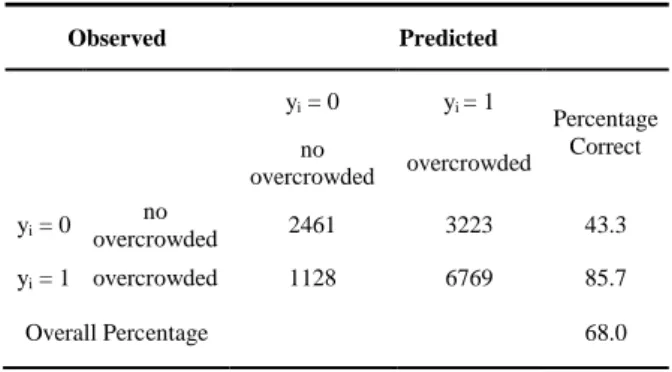
Now, let’s give a look to the classification table of the model, in Table 2.
Table 2. Classification Table*
Observed Predicted yi = 0 yi = 1 Percentage Correct no overcrowded overcrowded yi = 0 no overcrowded 2461 3223 43.3 yi = 1 overcrowded 1128 6769 85.7 Overall Percentage 68.0 *cut point 0.5.
By observing the classification table, one can appreciate that our model presents 1128 false positives. The false positives are the ones that considering a probability of 50% (the cut value is .500) were classified incorrectly in the prediction of being in an overcrowding situation (Yi=1). In other words, the proportion of false positives, which is 32.9%, represents the proportion of incorrect cases in the prediction of the group of being in overcrowding situation Yi=1. On the other hand, the number of households classified as false negative is 3223. These households are the ones classified incorrectly in the set of the predictions of not being in an overcrowding situation Yi=0. However, globally, the model presents a 68% of correct predictions which, for a probabilistic binary choice model is quite good. Indeed, this percentage of correct predictions can be consider as a measure of goodness of fit without taking credit of the R squares discussed below, in Table 3.
Table 3. Model Summary
Criterion Intercept Only Intercept and Covariates
-2 Log
likelihood 18465.075 16534.196 AIC 18467.075 16552.196 Cox & Snell R
Square .133
Nagelkerke R
Square .178
Regarding the value of the -2 Log likelihood when one considers the intercept and covariates, the estimation terminated at itineration 4 because parameter estimates change less than .001. This value of 16534.196 is considerably smaller than the one of 18465.075 obtained when only the intercept term is considered in the model. This diminishing in the -2 Log likelihood suggests that our variables contribute and give explanation power to the model. As a matter of fact, this guess is also verified due to the Akaike Information Criteria (AIC) which presents a decrease of 1914.879 when one considers the intercept and covariates with respect to only the intercept. Regarding the values of 13.3% and 17.8% obtained in the Cox & Snell and Nagelkerke R squares respectively, they can be consider quite acceptable since in this type of models the estimation is not based on maximizing the measure of goodness of fit like in the linear regression models.
5. CONCLUSIONS
It has been constructed a binary choice model with logit specification that allows to calculate the probability of being under overcrowding situation in the household considering as an overcrowded household in which there are more than three people per bedroom. Our empirical analysis, using data from Ecuador, indicates that a set of variables of the head of the household influence the probability of being in overcrowding situation. Particularly, it has been verified that the influence of the age of the household on the probability of being in overcrowding situation behaves as a concave function indicating that as the time passes the number of members in the household increases until certain point when it starts to decrease. In addition, it has been found that the regime of tenancy under which the household is living in the dwelling also affects the probability of being in an overcrowded household. Surprisingly, once the correct explanatory variables have been included in the model, our empirical analysis shows that there is no statistical significant evidence about the influence of the area, meaning being settled in the urban or rural side, on the probability of being in an overcrowded household.
Additionally, our findings also could have public policy implications. In that sense, considering that it has been characterized the fact of being in overcrowding situation based on a set of variables related to the head of the household, public policies can be addressed to overcome this condition. For example, housing credit policies can be addressed to the head of the household at the age in which there is more probability of being in overcrowding situation which would lead to improve living conditions of the entire household. Moreover, housing credit policies would affect the regime of tenancy of the household which can turn out in an increasing of wealth and welfare in the household.
Finally, this research opens the door for further studies. Considering the fact that in this paper authors have studied the factors that affect the probability of being in overcrowding situation in a developing country, afterwards one could study the dynamics of this social problem in developed countries and contrast the results, so structural
differences can be detected. Moreover, since now it is known what are the factors that contribute to increase the overcrowding probability, one could study the effects of it at a household level in further research then.
REFERENCES
Acosta, A (2012). Breve Historia Económica del Ecuador. Corporación Editora Nacional.
Baker, M D. Das, K. Venugopal, and P. Howden-Chapman (2008). Tuberculosis Associated with Household Crowding in a Developed country. Journal Epidemiol Community Health 62. p.p. 715–721.
Baldassare, M. (1978). Residential Crowding in Urban America. Berkeley: University of California Press.
Bongaarts, John (2001). Household Size and Composition in the Developing World in the 1990s. Population Studies, Vol. 55, No. 3 p.p. 263-279. Burch, T. (1970). Some Demographic Determinants of Average Household Size: An Analytic Approach. Demography, Vol. 7, No. 1. p.p. 61-69. Carnahan D. et al. (1974). Urbanization, Population Density and Overcrowding: the Quality of Life in Urban America. Social Forces 53. p.p. 62-72
Comisión Económica para América Latina y el Caribe CEPAL (2001). El Método de las Necesidades Básicas Insatisfechas (NBI) y su aplicación para América Latina. Santiago de Chile.
De Cabo, G. (2007). Diferencia y Discriminación Salarial por Razón de Sexo. Instituto de la Mujer. Madrid.
Galle, O. and W. Gove. (1978). Overcrowding, Isolation and Human Behavior: Exploring the Extremes in Population Distribution. Karl Tauber and James Sweet (eds.). Social Demography. P.p. 95-132.
Iglesias de Usel, J. (1993). Vivienda y Familia. In Garrido, L, Estrategias Familiares.
Instituto Nacional de Estadísticas y Censos (2006). Encuesta de Condiciones de Vida.
Lanjouw, P. and M. Ravallion (1995). Poverty and Household Size. The Economic Journal, Vol. 105, No. 433 p.p. 1415-1434
Lentini, M. (1997). El hacinamiento: La dimensión no visible del déficit habitacional. Boletin INVI 31. Volume 12. p.p. 23-32.
Marx, B and T. Stroker (2013). The Economics of Slums in the Developing World. The Journal of Economic Perspectives. Vol. 27, No. 4. p.p. 187-210. Puga, J. (1983). Consecuencias sociales del déficit habitacional en los sectores urbanos de mínimo ingreso. In Donald, J Vivienda Social – Reflexiones y experiencias.