Growth, polarization and poverty reduction in Africa in the past two decades

(1)

UNIVERSITÀ DEGLI STUDI DI MACERATA DIPARTIMENTO di Economia e Diritto

CORSO DI DOTTORATO DI RICERCA IN Metodi Quantitativi per la Politica Economica

CICLO XXXI

Growth, Polarization and Poverty Reduction in Africa in the Past

Two Decades

RELATORE DOTTORANDO

Chiar.mo Prof. Gallagati Marco Dott. Fabiani Michele

CORRELATORE

Chiar.mo Prof. Clementi Fabio

COORDINATORE

Chiar.mo Prof. Ciaschini Maurizio

(2)

a

Abstract

The present thesis observes the situation of growth, of inequality, from the point of view of polarization and poverty on the African continent in the past two decades.

The first part, starting from the evidence of low growth-to-poverty elasticity characterizing Africa, purports to identify the distributional changes that limited the pro-poor impact of the growth of the last two decades. Distributional changes that went undetected by standard inequality measures were not showing a clear pattern of inequality on the continent. A new decomposition technique is applied based on a non-parametric method—the “relative distribution”—and a clear distributional pattern affecting almost all analyzed countries is found. Nineteen of 24 countries experienced a significant increase in polarization, particularly in the lower tail of the distribution, and this distributional change lowered the pro-poor impact of growth substantially. Without this unfavorable redistribution, poverty could have decreased in these countries by an additional five percentage points.

The second part uses a set of national household surveys to provide the first estimates of the level of polarization and inequality for Sub-Saharan Africa as a whole over the period from 1997 to 2012. Save for a slight decline between 1997 and 2002, regional polarization steadily increased throughout the 2000s with greater polarization in the lower tail of the distribution than in the upper tail. This rise in regional polarization was mainly driven by increasing polarization between countries, meaning Sub-Saharan Africa tended to polarize spatially with the Southern cone countries performing above the average and Central African countries lagging behind.

The last part observes the polarization situation in three countries of North Africa, Tunisia, Morocco and Egypt, in the period between what is defined as the Arab spring using the methodologies seen above. The three countries experienced a significant increase in polarization, specifically in the lower part of the distribution.

(5)

d

Acknowledgements

First and foremost, I want to thank my supervisor, Professor Fabio Clementi. It has been an honor to be his first Ph.D. student. He was my mentor, the person who made me passionate about the subject, and without him, this work could not have existed. We shared these intense three years, and I will never stop thanking him for all the help I have been given.

I wish to thank Vasco Molini, Senior Economist of the World Bank Group. His contribution was fundamental for the realization of the entire work, he was always available for any advice and support, and it was an honor to have the opportunity to work side by side in Rabat. The most important thing is that, in both of them, I found not only inspiring and excellent professionals but also, from my point of view, two friends.

I want to thank the World Bank Group for allowing us to work with them and for the availability of data, a fundamental part of this thesis.

I want to thank Silvia, my other half, without which I would not have even started this path. She convinced me to start this journey, we shared every beautiful moment, and she supported me and encouraged me not to stop at every difficulty. Without her, I would not be here to write all this.

Finally, I want to send a big thank to my family who, with their tireless support, both moral and economic, have allowed me to arrive here in front of you today, contributing to my personal training.

(6)

e

List of Table

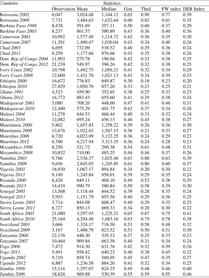
2.1: Main statistics of consumption, inequality and polarization for each country 25

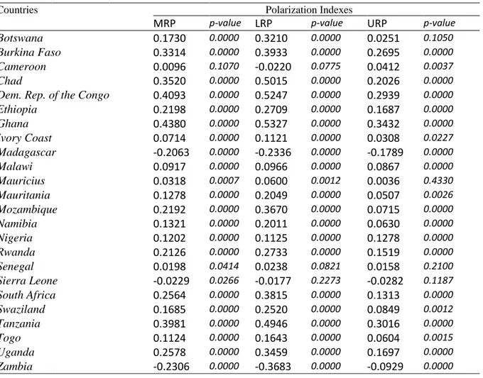
2.2: Polarization Indexes 31

3.1: Composition of benchmark years 56

3.2: Summary measures of Sub-Saharan African consumption distribution 63

3.3: Relative polarization indices 68

4.1: Main statistics of consumption, inequality and polarization for each country 79

4.2: Polarization Indexes 81

A.1: Growth and inequality elasticities by SSA country (headcount ratio and poverty

gap measure). 86

A.2 – Oaxaca-Blinder decomposition results, Burkina Faso 98

A.3 – Oaxaca-Blinder decomposition results, Cameroon 105

A.4 – Oaxaca-Blinder decomposition results, Ivory Coast 105

A.5 – Oaxaca-Blinder decomposition results, Ghana 106

A.6 – Oaxaca-Blinder decomposition results, Guinea 106

A.7 – Oaxaca-Blinder decomposition results, Mauritania 106

A.8 – Oaxaca-Blinder decomposition results, Mozambique 107

A.9 – Oaxaca-Blinder decomposition results, Niger 107

A.10 – Oaxaca-Blinder decomposition results, Nigeria 107

A.11– Oaxaca-Blinder decomposition results, Democratic Republic of Congo 108

A.12 – Oaxaca-Blinder decomposition results, Rwanda 108

(7)

f

List of Figures

Figure 1.1: GDP per capita and household consumption average growth rates:

1999-2014 6

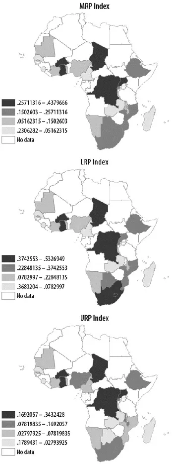
Figure 2.1: Relative consumption distribution for Ethiopia between 2000 and 2010 27 Figure 2.2: Relative consumption distribution for Ghana between 1991 and 2012 28 Figure 2.3: Relative consumption distribution for South Africa between 2005 and 2010 29 Figure 2.4: Relative polarization indices, geographical distribution 32 Figure 2.5: Variation in the poverty headcount ratio and decomposition into growth and redistribution components (Author method)

34 Figure 2.6 (a): Growth components compared (headcount ratio). 35 Figure 2.6 (b): Redistribution components compared (headcount ratio).

Figure 2.7 (a): Growth components compared (poverty gap) Figure 2.7 (b): Redistribution components compared (poverty gap)

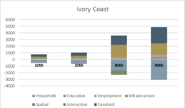
35 36 36 Figure 2.8: Oaxaca-Blinder decomposition results for Burkina Faso 44 Figure 2.9: Oaxaca-Blinder decomposition results for Cameroon 45 Figure 2.10: Oaxaca-Blinder decomposition results for Ivory Coast 45 Figure 2.11: Oaxaca-Blinder decomposition results for Ghana 46 Figure 2.12: Oaxaca-Blinder decomposition results for Guinea 46 Figure 2.13: Oaxaca-Blinder decomposition results for Mauritania 47 Figure 2.14: Oaxaca-Blinder decomposition results for Mozambique 47 Figure 2.15: Oaxaca-Blinder decomposition results for Niger 48 Figure 2.16: Oaxaca-Blinder decomposition results for Nigeria 48 Figure 2.17: Oaxaca-Blinder decomposition results for Democratic Republic of Congo 49 Figure 2.18: Oaxaca-Blinder decomposition results for Rwanda 49 Figure 2.19: Oaxaca-Blinder decomposition results for Senegal 50 Figure 3.1: Changes in the Sub-Saharan African distribution of consumption

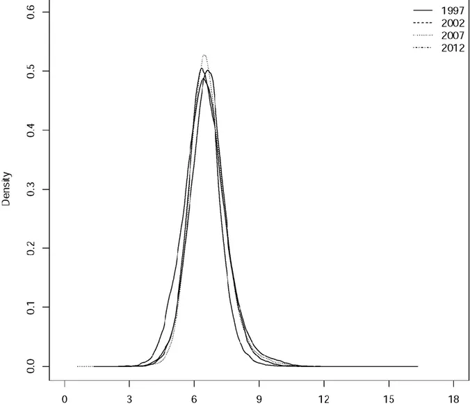
expenditure between 1997 and 2012 61

Figure 3.2: Relative consumption distribution for Sub-Saharan Africa between 1997 and

(8)

g

Figure 3.3: Location and shape decomposition of the relative consumption distribution

for Sub-Saharan Africa by sub-periods. 69

Figure 3.4: Relative polarization indexes by sub-periods. 70 Figure 3.5: Decomposition of Sub-Saharan African inequality and polarization into

differences between and within countries 72

Figure 3.6: The median-adjusted relative consumption distribution by sub-regions, 2012 to 1997

Figure 4.1: Parametric distributions from grouped data 73

Figure 4.2: Relative consumption distribution for Egypt between 2008 and 2015 80 Figure 4.3: Relative consumption distribution for Morocco between 2001 and 2013 83 Figure 4.4: Relative consumption distribution for Tunisia between 2005 and 2015 84 Figure 4.5: Relative distribution results, by subperiods 85

Figure 4.6: Polarization indexes, by subperiods 88

(9)

1

Chapter 1 Introduction

1.1 Preface

The questions of inequality and the distribution of income have an increasing interest in economic literature in recent years. From the introduction of the concept of the “Kuznets Curve”, the inverse-U shaped pattern of inequality introduced by Kuznets (1955), the trend in inequality linked to the economic growth of the post-war years in Western countries was very interesting. Kuznets theorized that, as a result of the economic growth of a country, the inequality first grew until it reached the peak and then fell.

The empirical validity of the “Kuznets Curve” has been investigated extensively, but the empirical results are different and contrasting. Atkinson (1999) shows that for different developed countries, the Gini index has different trends and increases in many cases. Piketty (2000, 2006) and Alvaredo (2009) argued that the Kuznets curve does not exist. The decline of inequality observed by Kuznets in the United States is not linear and depends on the Great Depression or by the two World Wars, for example.

From the economic crisis, the argument again started to be the center of the academic debate. Stiglitz (2012), in his book The price of inequality, emphasizes that inequality is rooted in the current market economy, which has led to increased distances between individuals. Thomas Piketty, in recent years, through different works such as The capital of XX century (2013), draws attention to the issues of inequality and highlights its problem in the last decades. The question of polarization of income is of interest to observe inequality from a different point of view. Over the last two decades, the issue of polarization has gained importance in the analysis of income distribution. Notwithstanding the pains the polarization literature has suffered to distinguish itself from pure inequality measurement—see e.g. Foster and Wolfson (1992, 2010), Levy and Murnane (1992), Esteban and Ray (1994), and Wolfson

(10)

2

(1994, 1997)—it has become widely accepted that polarization is a distinct concept from inequality.

Broadly speaking, the notion of polarization is concerned with the disappearance of the middle class, which occurs when there is a tendency to concentrate in the tails—rather than the middle—of the income distribution. One of the main reasons for looking at income polarization this way, which is usually referred to as “bi-polarization”, is that a well-off middle class is important to every society because it contributes significantly to economic growth as well as to social and political stability (e.g. Easterly, 2001; Pressman, 2007; Birdsall, 2010). In contrast, a society with a high degree of income polarization may give rise to social conflicts and tensions. Therefore, in order for such risks to be minimized, it is necessary to monitor the economic evolution of the society using indexes that look at the dispersion of the income distribution from the middle toward either or both of the two tails.1 Measures of income polarization that correspond to this case have been proposed in the literature by Foster and Wolfson (1992, 2010), Wolfson (1994, 1997), Wang and Tsui (2000), Chakravarty and Majumder (2001), Rodríguez and Salas (2003), Chakravarty et al. (2007), Silber et al. (2007), Chakravarty (2009), Chakravarty and D’Ambrosio (2010), Lasso de la Vega et al. (2010), and others.

A more general notion of income polarization (Esteban and Ray, 1994) regards the latter as the “clustering” of a population around two or more poles of the distribution, irrespective of where they are located along the income scale. The notion of income polarization in a multi-group context is an attempt at capturing the degree of potential conflict inherent in a given distribution (see Esteban and Ray, 1999, 2008, 2011). The idea is to consider society as an amalgamation of groups, where the individuals in a group share similar attributes with fellow members (i.e. have a mutual sense of “identification”), but in terms of the same attributes, they

1_{More precisely, there are two characteristics that are considered as being intrinsic to the notion of bi-polarization.}

The first one, “increased spread”, implies that moving from the central value (median) to the extreme points of the income distribution makes the distribution more polarized than before. In other words, increments (reductions) in incomes above (below) the median will widen the distribution: Extend the distance between the groups below and above the median and hence increase the degree of bi-polarization. On the other hand, “increased bi-polarity” refers to the case where incomes on the same side of the median get closer to each other. Since the distance between the incomes below or above the median has been reduced, this is assumed to increase polarization. Thus, bi-polarization involves both an inequality-like component, the “increased spread” principle, which increases both inequality and polarization, and an equality-like component, the “increased bi-polarity” criterion, which increases polarization but lowers any inequality measure that fulfills the Pigou-Dalton transfer principle—the requirement under which inequality decreases when a transfer is made from a richer to a poorer individual without reversing their pairwise ranking. This shows that although there is complementarity between polarization and inequality, there are differences as well. See the references cited in the main text for a thorough discussion.

(11)

3

are different from the members of the other groups (i.e. have a feeling of “alienation”). Political or social conflict is, therefore, more likely, the more homogeneous and separate the groups are, that is when the within-group income distribution is more clustered around its local mean, and the between-group income distance is longer. In addition to Esteban and Ray (1994), indexes regarding the concept of income polarization as conflict among groups have been investigated, among others, by Gradín (2000), Milanovic (2000), D’Ambrosio (2001), Zhang and Kanbur (2001), Reynal-Querol (2002), Duclos et al. (2004), Lasso de la Vega and Urrutia (2006), Esteban et al. (2007), Gigliarano and Mosler (2009), and Poggi and Silber (2010).

Much of the literature so far considered has analyzed summary measures of income polarization. Another strand uses kernel density estimation and mixture models in order to describe changes in polarization patterns over time, not just of personal incomes (as in Jenkins, 1995, 1996; Pittau and Zelli, 2001, 2004, 2006; Conti et al., 2006) but also of the cross-country distribution of per capita income (see Quah, 1996a,b, 1997; Bianchi, 1997, Jones, 1997; Paap and van Dijk, 1998; Johnson, 2000; Holzmann et al., 2007; Henderson et al., 2008; Pittau et al., 2010; Anderson et al., 2012; and others). The analysis of the shape of the income distribution provides a picture from which at least three important distributional features can be observed simultaneously (Cowell et al., 1996): income levels and changes in the location of the distribution as a whole; income inequality and changes in the spread of the distribution; clumping and polarization; changes in patterns of clustering at different modes.

Finally, a rather recent (yet non-parametric) approach that combines the strengths of summary polarization indexes with the details of distributional change offered by the kernel density estimates—the so-called “relative distribution”—has been employed by Alderson et al. (2005), Massari (2009), Massari et al. (2009a,b), Alderson and Doran (2011, 2013), Borraz et al. (2013), Clementi and Schettino (2013, 2015), Guangjin (2013, 2014), Molini and Paci (2015), Nissanov and Pittau (2016), Petrarca and Ricciuti (2016), Nissanov (2017), Clementi et al. (2017, 2018b), and Kabudula et al. (2017) to assess the evolution of the middle class and the degree of income polarization in a number of low- to high-income countries around the world.

Not much discussed, but growing in recent years, is inequality in developing countries, specifically, in Africa. This is important to observe, for example, if there is a connection between inequality and different problems about the continent, from the question of poverty to

(12)

4

economic growth to social and violent conflicts. The central objective of this thesis is to propose an in-depth picture of the distribution of income in Africa from different points of view.

1.2 The non-inclusive growth of African economy and the

problem of inequality

Despite experiencing stable and sustained growth for almost two decades, several Sub-Saharan Africa (SSA) countries have not experienced a commensurate reduction in poverty.

Recent estimates, based on an international poverty line of US$1.90 (in 2011 PPP U.S. dollars), suggest that poverty declined only by 23 percent between 1990 and 2012 (from 56 percent to 43 percent) (Beegle et al., 2016). This rate is much lower than those experienced by countries with similar growth rates and similar poverty rates in other regions. The World Bank (2018) calculates that in a typical non-African developing country, where 50 percent of the population is living below the poverty line, a one percent yearly growth in GDP led to a reduction of 0.53 percentage points a year in the incidence of poverty. In contrast, the same one percent per capita GDP growth in a typical African country with the same poverty incidence reduced poverty by only 0.16 percentage points.

The two general explanations for this lower growth poverty-elasticity in Africa are: questioning the veracity of the recent African economic boom (the so-called African miracle); looking at the role of inequality. Jerven (2013, 2015) has provided evidence on the problems afflicting GDP calculations in Africa and argued that for many SSA countries, the recent high growth is merely statistical or in other words, a feature of adding the informal sector that previously was not counted (Jerven, 2015). Since growth is overstated, it is thus not surprising that poverty did not fall so rapidly.

Another interesting study regarding the aspect of growth in the Sub-Saharan African economy is proposed by Rodrik (2016). The author underlines the exogenous characteristic of the economic growth of the last two decades, guided from the high price of the commodities and low interest rate. Furthermore, the author underlines the importance of structural changes in the policy of African countries such as the initiation of reforms that have led to the openness of international trade and the end of numerous conflicts.

(13)

5

Moreover, the author shows that in order to have an effective "miraculous growth", countries must invest in the fundamentals (human capital, education) and at the same time, carry out a structural transformation towards the modern / manufacturing sector. In this case, however, the situation is not rosy for the African countries. In fact, both the share of employees in the industry and its incidence on GDP remain low, even lower than in the 1970s: in practice, we are witnessing a de-industrialization, although many countries remain too poor to have it, unlike what is happening in Asian countries.

Figure 2.1 compares the average growth of annual GDP per capita and the average consumption2_{growth from available household surveys; consumption is the welfare measure}

typically used to calculate poverty rates, growth is the factor that really matters in poverty reduction (Adams, 2004; McKay, 2013). Indeed, the discrepancy between GDP per capita growth and household consumption growth is higher in SSA than in the rest of the developing world. SSA, in fact, registers an average annual growth of household consumption of about 1.02 percent per year, not much lower than the South Asia Region (SAR) and slightly higher than in Latin America. Therefore, household consumption increased in SSA similarly to other developing regions, but poverty still declined slower.

(14)

6

Figure 1.1: GDP per capita and household consumption average growth rates: 1999-2014. The abbreviations refer to SSA= Sub-Saharan Africa; LAC= Latin America and the Caribbean; EAP= East Asia Pacific; SAR= South Asian Region; EAC= Eastern Europe and Central Asia.

Regarding inequality, the literature has debated its relationship with growth and poverty. Dollar and Kraay (2002) show that all income groups tend to benefit proportionally from increases in economic growth and that income distribution does not really matter for poverty reduction. Bourgignon (2003) and Ravallion (2007) find that inequality reduces the poverty-reducing effects of economic growth. Thorbecke (2013) argues that the combination of high endemic poverty and inequality is, in general, responsible for the low growth elasticity of poverty. High initial poverty and inequality directly reduces the growth rate but also indirectly the poverty-reducing effect of this growth. Looking at SSA, Fosu (2009, 2015) finds that economic growth reduces poverty while growth elasticity is a decreasing function of initial inequality. Therefore, the low elasticity registered in SSA in the last two decades could potentially be attributed to an increase in inequality that limited the pro-poor content of growth. Unfortunately, when measured with standard indicators like the Gini index or Theil index, there is no clear evidence of an increase in inequality in the last two decades. Pinkovskiy and Sala-i-Martin (2010) sustain that from the 1990s, inequality declined significantly in Sub-Saharan Africa, with a reduction of around three percent for the entire area. However, the

(15)

7

authors show that this reduction brought the Gini index back to the same levels as in the early 1970s.

Chotikapanich et al. (2014) find different results in ten selected countries from the 1990s to 2000s: in six countries they observe increases in inequality (i.e. South Africa and Ghana), while a marginal decrease or inverted U-shape is observed in four. Fosu (2014) finds that from the mid-1990s to the late 2000s, the Gini index grew in nine countries but dropped in thirteen and remained constant in one. Beegle et al. (2016), analyzing the SSA countries for which there are two comparable surveys, conclude that about half of them experienced a decline in inequality while the other half saw an increase.

Similar contrasting results are shown by Cornia et al. (2017) where, for the same period but for a larger sample of countries, four different trends of the Gini index are observed: for thirteen countries, there is a decrease in inequality, for seven countries, there is an increase, for four countries, an inverted U-shaped is observed, and a U-shaped is seen in five.

At first glance, therefore, there is no clear pattern in SSA that can explain the low elasticity of poverty through increasing inequalities. From a distributional point of view, it is still unclear why growth does not translate into greater household consumption at the bottom of the income distribution, at rates comparable with those experienced in other regions of the world (Christaensen et al., 2014; Thorbecke, 2013).

To answer at the previous problems, the first about the measures of inequality in Sub-Saharan Africa and the second about how the inequality affects the reduction of poverty, the first chapter proposes two different approaches, each one regarding one of the two items.

The first one aims to evaluate the distribution of wealth not only by observing inequality by using the standard measures like Gini Index or Theil index but also analyzing the polarization of the consumption with the method of relative distribution (Handcock and Morris, 1998, 1999). The polarization of income can be defined as the clustering of the population around two or more poles of the distribution (Esteban and Ray, 1994).

The relative distribution method is not well known but has already been used in several studies to observe the distribution of income in the countries and their polarization.

Clementi et al. (2015) use this method to observe the evolution of the distribution in Nigeria after the significant increase in GDP in the 2000s and how this change has emptied the middle class. The authors observe that the growth that occurred was not inclusive but led to an increase in polarization with a change in distribution. This change led to an emptying of the

(16)

8

middle class and to a concentration of households in the two tails of the distribution. This distributional change was not captured by standard measures of inequality, such as the Gini index.

Nissanov and Pittau (2015) use the same method to observe changes in income distribution in Russia between the 1990s and 2000s. Contrary to standard measures of inequality, the authors show a declining of the middle class and a significant increase in polarization in the lower tail, in the period 2000-2008. They underline the fact that this change is caused by the failure of the labor market in the country during the economic crisis. In this period, in fact, members of the middle class changed work, experiencing wage reductions.

Alderson et al. (2005) analyze the polarization trend in 16 core countries in the LIS (Luxembourg Income Study) dataset. In seven countries, like the United Kingdom, the United States and Italy, the authors observed an increase in inequality and polarization. In the other seven countries, the changes are modest, positive or negative, and heterogeneous. In Sweden and Canada, the inequality and polarization decline, with a significant shift of the population in the lower tail to the middle class.

In the second approach, a novel method to decompose the effect that changes in the distribution have on the reduction of poverty is proposed. Differently from the previous approach (Datt and Ravallion, 1992), this method is polarization-poverty and growth decomposition based. In their paper, Datt and Ravallion (1992) fix their model so that the level of poverty can change by two factors: a change in the average income compared to the poverty line (growth effect) or a change in the relative inequality (redistribution effect). Applying their model for India and Brazil, they observe that a negative redistributive effect (increase in inequality) leads to a negative effect on the reduction of poverty.

1.3 A global overview: An analysis of polarization without the

barriers

Recently, there is considerable interest in the economic literature in the level of relative inequality of incomes found among all people in the world regardless of their country of residence. Notable recent contributions include, among others, Anand and Segal (2008, 2015), Atkinson and Brandolini (2010), Bourguignon (2017), Bourguignon and Morrison (2002),

(17)

9

Lakner and Milanovic (2015), Milanovic (2002, 2005, 2012, 2016), and Niño-Zarazúa et al. (2017). The predominant methodology involves constructing a distribution of income of all the citizens of the world, using national accounts and/or survey data. Inequality is subsequently measured based on this global distribution of income.

As it emerges from most of these studies, in the last 30 years – the so-called globalization era – the global income distribution switched from a bi-modal to a unimodal distribution. This change occurs under the effect of two interrelated processes: an increase in inequality within-country and a fast decline of inequality between-countries (Milanovic, 2010; Luiten van Zanden et al., 2013). Thanks to an unprecedented period of increasing interconnectedness between domestic economies, the global income distribution has evolved away from the ‘twin peaks’ identified by Quah (1996) into a less polarized one (Roope, 2018).

Regional distributions tend to mirror the global one. Luiten van Zanden et al. (2013) document a generalized decline in the between-country inequality concomitant to the economic integration within the region. In different periods, this applies to Western Europe, North America, Latin America, and Eastern Asia. Sub-Saharan Africa represents a notable exception since throughout the twentieth century, the between-country inequality does not decrease. Starting from the 1980s, it increases (Luiten van Zanden et al. 2013), and this tendency protracts to the first decade of 2000 (Jirasavetakul and Lakner, 2016). From this evidence, it can be inferred that SSA looks like a highly polarized region; there are some relatively successful economies (predominantly in the Southern cone) and a big cluster of unsuccessful ones, recording among the lowest GDP per capita in the world. Be that as it may, there is a limited analysis that explicitly analyzes polarization in SSA.

Following Milanovic (2005) and Anand and Segal (2008), it is possible to define four concepts of the global distribution of income and their level of inequality based on the population unit and welfare concepts. The first one is the distribution of income by country. In this case, the “population unit” is the country and the “income concept” is the (total) national income of the country. This approach does not consider the dimension of the population of the country, and the differences are based only on the wealth of the country in its entirety.

In the second concept, the population unit remains the country, but in this case, the measure to observe the well-being is the national income per capita.

(18)

10

The third concept uses the national income per capita, but the population unit is the individual. In this case, the population dimension of each country is important because in observing a global distribution, every nation will have its specific weight.

The fourth concept considers both the individual and household and is considered the per-capita income of the individual or household to which the individual belongs. This approach allows us to observe the distribution of income (or consumption) and inequality in a similar way to the analyses carried out within individual countries.

The last concept is actually the one most used in global inequality literature.

Milanovic (2005) constructs inequality estimates over time for a common sample of countries, using 345 national surveys. The author builds three benchmark years (1988, 1993, 1998). For his analysis of the distribution within countries, he uses the deciles, assuming that the individuals within them have the same income/consumption. The results show that the inequality (Gini and Theil indexes) rises between 1988 and 1993 and declines between 1993 and 1998 but remains at a higher level with respect to 1988. Very interesting is the decomposition of indexes that shows that between-country inequality is the biggest part of total inequality (between 71 and 83 per cent) and remains stable over time.

Jirasavetakul and Lakner (2016) improve upon research about global inequality focusing on Sub-Saharan Africa. In this case, the authors created a global survey for specific benchmark years, following the example of Milanovic (2012) and Lakner and Milanovic (2015). Country-year consumption distribution is derived by ﬁtting a parametric Lorenz curve to the decile shares. The authors find a rise in regional inequality, which is driven by increasing inequality between-countries with an increase in the difference in living conditions.

Polarization is an appealing alternative indicator to inequality as a measure of changes in the welfare distribution. While inequality provides an indication of the overall dispersion of a distribution, polarization considers how distributional changes affect the income or consumption distribution between subgroups of society. More specifically, it is interesting how the dynamic process leads to the shrinkage of the middle class, the group of people in the center of the distribution, relative to the (two) groups on both extreme tails of the distribution (see, for instance, Foster and Wolfson, 1992 and Wolfson, 1994, 1997). Framing the problem using Duclos et al.’s (2004) formulation, polarization can be intended as the combination of two opposite forces: the “identification” within two or more groups and “alienation” or increasing (socio-economic) distance between the same groups.

(19)

11

While polarization analysis is typically undertaken at the country level, in the third chapter it is argued that there are good reasons to look at polarization at the regional level.

First, as pointed out by Roope et al. (2018), in an interconnected world, there is a clear parallel between the positive impact on economic growth and social cohesion that a domestic middle class has on a global/regional middle class. SSA, however, saw its middle class growing much slower than in the rest of the developing world (AfDB, 2011) and much less socio-economic integration. Internal tariffs reduced slower than in other regions, free mobility of goods and people is far from being achieved (UN, 2010; World Bank, 2011), and it is very difficult to reach a political consensus on a common economic agenda. This fragmentation, if not caused by, certainly in on par with the increasing economic polarization characterizing the region.

Second, polarization is strongly linked to the emergence of internal conflicts and civil wars (Esteban and Ray, 1999, 2008, 2011). Whereas these conflicts in SSA manifested typically at country level (Azam, 2001, 2006), the recent conflict episodes in the Sahelian belt (Mali, Niger, Northern Nigeria, Burkina Faso and Chad) or in the Great Lakes region (Burundi, Rwanda, Uganda and DRC) show that they can easily escalate at the sub-regional level. This likely is because, in presence of fragile states, the mechanisms that determine the identification/alienation duality can transcend national borders; ethnic or religious allegiances (Basedau et al., 2016; Allansson et al., 2017) can be a much stronger element of identification (and alienation from compatriots) than national identity. Just looking at the country level data, we argue, does not fully capture the full picture, while a regional perspective, we think, sheds some additional light, and the first step is clearly having a good sense of regional polarization patterns.

In the second chapter, an analysis of the polarization in Sub-Saharan Africa without considering the barriers and “global” distribution of consumption for the area, like in Jirasavetakul and Lakner (2016), are realized. The new significant elements introduce, with respect to the previous studies, are, firstly, are used directly the data from household surveys, combined to obtain a unique survey for determined benchmark years.

Secondly, the indexes are decomposed to see the composition of within-country and between-countries inequality and finally breaking down polarization, to see the territorial concentration of consumption in the area and observe which sub-areas compose the deciles of distribution.

(20)

12

1.4 The North African countries and the Arab Spring: a different

perspective of inequality

In the last part of this thesis, we will analyze the situation of the North Africa countries, specifically Morocco, Tunisia and Egypt. In the last years, this region has been the scene of massive protests by the population, which in some cases, evolved into violent conflicts. These events are known as the “Arab Spring”.

Economic literature started to observe the situation of income distribution and inequality in MENA countries and if the trend of inequality can be linked to revolutions. About this question, there are two different approaches.

The first sustained that the inequality decline in the region could not be the cause of the revolution.

Devarajan and Ianchovinchina (2017) sustain that the revolts in the Arab countries and inequality are disconnected. The authors find that consumption inequality is low and declines in the 2000s and remains lower than in the rest of the world. Following Hassine (2015), the authors show that total expenditure inequality declined in Tunisia, Egypt and Jordan, and in the other MENA countries that show an increase in the Gini index, it remains moderate.

The authors identified that with the fall of individuals’ welfare such as quality of life, expectations about the future or perceptions of declining standard of living caused social conflicts, and subsequently, the riots. All this was due to a change in the “social contract” in the MENA countries. In the past, the government was the main employer, provided free access to public services, and subsidized the purchases of goods. In the 2000s, this situation has not been sustainable, and governments have started to withdraw from the labor market and offer fewer subsidies.

Similar conclusions are provided by Hlasny and Verme (2013) for Egypt. The authors impute top income on the data derived from the Household Surveys, find a good quality of Egyptian expenditure data, and compare the consumption inequality between Egypt and another 107 countries, demonstrating that inequality in Egypt is lower. They sustained, like the previous study, that the riots in Egypt derived from social problems and not from income inequality.

(21)

13

The second group of research sustained, instead, that inequality in MENA countries is higher respective to other regions, and this may have influenced the riots during the “Arab Spring”.

Alvaredo et al. (2018), combining Household survey and tax data, show that the top 10 per cent’s share rises 64% in the Middle East between the 1990s and 2010s, compared to 37% in Western Europe or 39% in all of Europe. From another point of view, they observe that the between-countries inequality in the area is very high, with oil-rich countries that represent only 15% of the Middle East population, receive more than 40% of the whole Middle East income.

Lakner et al. (2016) come back to the question of underestimation of top income. Top income is under-estimated when using only the Household survey data (Atkinson et al., 2011). One way to estimate the top tail of the income distribution is using data from income tax records, but in less developed countries, these data are limited. For this reason, the authors used data on house price to estimates the top income of the distribution in Egypt. Using this method, the authors find that inequality is underestimated in Egypt, with the Gini index in 2009 rising at 47%, with respect to a survey estimate of 36.4%.

In this chapter, the analysis is focused on three countries of North Africa: Morocco, Tunisia, and Egypt. These countries experienced a different situation during the “Arab Spring”. Compared to the situation in Tunisia and Egypt, the uprisings did not result in violent riots in Morocco.

Like in previous chapters, we observe the differences among these three countries in terms of inequality. Besides inequality, the polarization of consumption will also be observed. In measuring polarization, we use the same methods observed in previous chapters: the Forster-Wolfson Index (Forster and Forster-Wolfson, 1992, 2010), the Duclos-Esteban-Ray Index (Duclos et al., 2004), and the method of relative distribution (Handcock and Morris, 1998, 1999).

Moreover, a parametric imputation estimation is used for the distribution of consumption of Tunisia in 2015. For this year, only grouped data from the national household survey are available.

(22)

14

Chapter 2 Polarization in Sub-Saharan Africa

3

2.1 Preface

The central argument of this chapter is that significant distributional changes against poverty reduction have, in fact, taken place in most of SSA countries we analyze. These changes affected predominantly the lower part of the welfare distribution and went undetected by standard inequality measures. The reason is simple. Summary measure like Gini don’t assign a weight to the different percentiles; if a pro inequality change in one part of the distribution is more than compensated by a pro-equality change in the rest of the distribution, Gini will decline. The distributional changes, however, that matter most for poverty reduction are those localized in the lower part of the distribution but can be detected only if we are able to focus on this part only.

To analyze these changes, in this chapter is applied a different type of decomposition based on the “relative distribution” method (Handcock and Morris, 1998, 1999). The advantage of this method consists of providing a non-parametric framework for taking into account all the distributional differences that could have affected the variation in the poverty rate and countered the pro poor effect of growth. In this way, it enables to summarize multiple features of the welfare distribution that a standard decomposition based on summary inequality measures would have not detected (Datt and Ravallion, 1992; Kolenikov and Shorrocks, 2005).

The chapter is organized as follow: Section 2 explicates the methodology used for analyzing polarization, the relative distribution method, and the approach to decompose growth and decomposition effect, that influence the reduction of poverty. Section 3 introduces the data used and the summary statistics. Section 4 provides the results of relative distribution method and the decomposition. Section 5 introduces the Oaxaca-Blinder decomposition method, to

3_{This chapter, modified and adapted according to needs, has been published as World Bank Working Paper in}

(23)

15

observe the impact of the covariates on the distribution of household consumption. Section 6 provides a summary and conclusions.

2.2 Methodology

2.2.1 Polarization: an introduction

Over the last two decades, the issue of polarization has gained increasing importance in the analysis of income distribution (Foster and Wolfson, 1992; Levy and Murnane, 1992; Esteban and Ray, 1994; Wolfson; 1994, 1997) and now it seems to be widely accepted that polarization is a distinct concept from inequality.

A general notion of income polarization (Esteban and Ray, 1994) regards it as “clustering” of a population around two or more poles of the distribution, irrespective of where they are located along the income scale. The notion of income polarization in a multi-group context is an attempt at capturing the degree of potential conflict inherent in a given distribution (see Esteban and Ray, 1999, 2008, 2011). The idea is to consider society as an amalgamation of groups, where the individuals in a group share similar attributes with its members (i.e. have a mutual sense of “identification”) but they are different from the members of the other groups (i.e. have a feeling of “alienation”).

Political or social conflict is therefore more likely the more homogeneous and separate the groups are, that is when the within-group income distribution is more clustered around its local mean and the between-group income distance is longer (see, inter alia, Gradín, 2000, Milanovic, 2000, D’Ambrosio, 2001, Zhang and Kanbur, 2001, Reynal-Querol, 2002, Duclos et al., 2004, Lasso de la Vega and Urrutia, 2006, Esteban et al., 2007, Gigliarano and Mosler, 2009, and Poggi and Silber, 2010).

A different approach regards the concept of bi-polarization (Foster and Wolfson, 1992, 2010): in this case, the two poles are formed on the two sides of the median, in the tails of distribution. The principal reason for looking at polarization this way is that a large and wealthy middle class contributes to economic growth in many ways, and hence is important to every society.

(24)

16

The middle class occupies the intermediate position between the poor and the rich and a society with thriving middle class contributes significantly to social and political stability as well (Easterly, 2001; Pressman, 2007).

There are two characteristics that are considered as being intrinsic to the notion of bi-polarization: increased spread implies that moving from the central value (median) to the extreme points of the income distribution make the distribution more polarized

than before; increased bi-polarity refers to the case where incomes on the same side of the median get closer to each other.

Thus, bi-polarization involves both an inequality-like component, the “increased spread” principle, which increases both inequality and polarization, and an equality-like component, the “increased bi-polarity” criterion, which increases polarization but lowers inequality.

2.2.2 Relative distribution

The use of summary measures of income polarization is common in literature. The approach used in this paper, the so-called “relative distribution”, combines the strengths of summary polarization indices with details of distributional change that the kernel density estimates yields. The relative distribution method has been employed by Alderson et al. (2005), Massari (2009), Massari et al. (2009a,b), Alderson and Doran (2011, 2013), Borraz et al. (2013), Clementi and Schettino (2013, 2015), Clementi et al. (2017, 2018), Molini and Paci (2015), Petrarca and Ricciuti (2016), Nissanov and Pittau (2016), and Nissanov (2017).

More formally,4_{let Y}

0 be the income variable for the reference population and Y the income variable for the comparison population. The relative distribution is defined as the ratio of the density of the comparison population to the density of the reference population evaluated at the relative data r:

𝑔(𝑟) = 𝑓(𝐹0−1(𝑟))

𝑓0(𝐹0−1(𝑟))

= 𝑓(𝑦𝑟)

𝑓0(𝑦𝑟), 0 ≤ 𝑟 ≤ 1, 𝑦𝑟 ≥ 0, (2.1)

4_{Here we limit ourselves to illustrating the basic concepts behind the use of the relative distribution method.}

(25)

17

where f (·) and f0 (·) denote the density functions of Y and Y0, respectively, and yr = 𝐹₀−1(𝑟) is the quantile function of Y0. When no changes occur between the two distributions, g(r) has a uniform distribution; a value of g(r) higher (lower) than 1 means that the share of households in the comparison population is higher (lower) than the corresponding share in the reference population at the rth_{quantile of the latter.}

One of the major advantages of this method is the possibility to decompose the relative distribution into changes in location and changes in shape. The decomposition can be written as: 𝑓(𝑦𝑟) 𝑓⏟0(𝑦𝑟) 𝑂𝑣𝑒𝑟𝑎𝑙𝑙 = 𝑓𝑜𝐿(𝑦𝑟) 𝑓0(𝑦𝑟) ⏟ 𝐿𝑜𝑐𝑎𝑡𝑖𝑜𝑛 × 𝑓(𝑦𝑟) 𝑓⏟ 0𝐿(𝑦𝑟) 𝑆ℎ𝑎𝑝𝑒 . (2.2)

F0L (yr) is the median-adjusted density function:

𝑓0𝐿(𝑦𝑟) = 𝑓0(𝑦𝑟+ 𝜌), (2.3)

where the value 𝜌 is the difference between the medians of the comparison and reference distributions—alternative indices like the mean and/or multiplicative location shift can also be considered.

The first ratio term in the right-hand side of Equation (2) is an estimate of the “location effect”, i.e. the pattern that the relative distribution would have displayed if there had been no change in distributional shape but only a location shift of the consumption distribution over time. When the median-adjusted and unadjusted reference populations have the same median, the ratio for location differences will have a uniform distribution. Conversely, when the two distributions have different median, the location effect is increasing (decreasing) if the comparison median is higher (lower) than the reference one.

The second term (the “shape effect”) represents the relative distribution net of the location effect and is useful to isolate movements (re-distribution) occurred between the reference and comparison populations. For instance, one could observe a shape effect with some sort of (inverse) U-shaped pattern if the comparison distribution is relatively (less) more spread around

(26)

18

the median than the median-adjusted reference distribution. Thus, it is possible to determine whether there is polarization of the consumption distribution (increases in both tails), “downgrading” (increases in lower tail), “upgrading” (increases in the upper tail) or convergence towards the median (decreases in both tails).

The relative distribution approach also includes a median relative polarization index, which is a measurement of the degree to which the comparison distribution is more polarized than the reference one:

𝑀𝑅𝑃 = 4 𝑛 (∑ |𝑟𝑖 − 1 2| 𝑛 𝑖=1 ) − 1. (2.4)

The values of the MRP index ranges between -1 and 1: positive values represent more income polarization and negative values represent less polarization; a value of 0 indicates no differences in distributional shape. The MRP index can be additively decomposed into the lower

relative polarization index and the upper relative polarization index, enabling one to distinguish

downgrading from upgrading. The two indices can be defined as:

𝐿𝑅𝑃 = 8 𝑛 (∑ ( 1 2− 𝑟𝑖) 𝑛/2 𝑖=1 ) − 1 (2.5) 𝑈𝑅𝑃 = 8 𝑛 ( ∑ (𝑟𝑖 − 1 2) 𝑛 𝑖=𝑛₂+1 ) − 1 (2.6)

with MRP= (1/2) (LRP + URP). As the MRP, LRP and URP range from -1 to 1 and equal 0 when there is no change.

(27)

19

2.2.3 Decomposition method

The relative distribution is a well-established approach to distributional analysis, whereas novel is the polarization-poverty and growth decomposition we develop for showing how the distributional changes we observed in many SSA countries have effectively limited the impact of growth on poverty reduction.

In general terms, poverty 𝑃(𝑧, 𝜇, 𝐿) is expressed in terms of poverty line, 𝑧, mean income level, 𝜇, and the Lorenz curve, 𝐿, representing the structure of relative income inequalities. Assuming the poverty line is fixed at a given level, poverty is given by 𝑃(𝜇, 𝐿). The total change in poverty, ∆𝑃, is then decomposed into two components. The first component is the growth component due to changes in the mean income while holding the Lorenz curve constant at some reference level, and the second a redistribution component due to changes in the Lorenz curve while keeping the mean income constant at some reference level.

Following Heshmati (2007), one can compute growth and inequality decompositions in various ways. Kakwani and Subbarao (1990) introduced the following decomposition:

∆𝑃 = 𝑃(𝜇₁, 𝐿₁) − 𝑃(𝜇₀, 𝐿₀) = [𝑃(𝜇_⏟₁, 𝐿₀) − 𝑃(𝜇₀, 𝐿₀)] 𝐺 + [𝑃(𝜇_⏟₁, 𝐿₁) − 𝑃(𝜇₁, 𝐿₀)] 𝑅 , (2.7)

where 𝜇 and 𝐿 are mean income and the Lorenz curve characterizing the distribution of income. The subscripts 0 and 1 denote the two (consecutive or non-consecutive) initial and final periods of observation, and 𝐺 and 𝑅 are contributions from the growth and redistribution components.

Jain and Tendulkar (1990) suggested an alternative formulation:

∆𝑃 = 𝑃(𝜇1, 𝐿1) − 𝑃(𝜇0, 𝐿0) = [𝑃(𝜇⏟ 1, 𝐿1) − 𝑃(𝜇0, 𝐿1)] 𝐺

+ [𝑃(𝜇⏟ 0, 𝐿1) − 𝑃(𝜇0, 𝐿0)]

𝑅 (2.8)

which differs from the previous decomposition by the reference point (base year versus final year) that is initially chosen for computation of growth and redistribution components.

Kakwani (2000) suggested a simple averaging of both the growth and inequality components from Equations (7) and (8), which is:

(28)

20 ∆𝑃 =1 2{[𝑃(𝜇1, 𝐿0) − 𝑃(𝜇0, 𝐿0)] + [𝑃(𝜇1, 𝐿1) − 𝑃(𝜇0, 𝐿1)]} ⏟ 𝐺 +1 2{[𝑃(𝜇1, 𝐿1) − 𝑃(𝜇1, 𝐿0)] + [𝑃(𝜇0, 𝐿1) − 𝑃(𝜇0, 𝐿0)]} ⏟ 𝑅 (2.9)

Datt and Ravallion (1992) found the above decompositions of poverty changes as being time path dependent, arising through and dependent on the choice of reference levels. To make the changes path independent they proposed adding an extra residual 𝐸 as follows:

∆𝑃 = 𝑃(𝜇₁, 𝐿₁) − 𝑃(𝜇0, 𝐿0) = [𝑃(𝜇⏟ 1, 𝐿0) − 𝑃(𝜇0, 𝐿0)] 𝐺

+ [𝑃(𝜇⏟ ₁, 𝐿₁) − 𝑃(𝜇1, 𝐿0)] 𝑅

+ 𝐸 (2.10)

The residual in (10) can be interpreted as the difference between the growth (redistribution) components evaluated at the terminal and initial Lorenz curves (mean incomes), respectively.

Another strand of the research literature has used panel data to explore cross-country differences in the growth-inequality-poverty relationship. Some recent contributions following this approach include Kalwij and Verschoor (2007) and Fosu (2015, 2017a, 2017b, 2018). These authors decompose poverty changes into growth and inequality (redistribution) effects as follows: ∆ln𝑃_𝑖𝑡 = 𝜀_⏟_𝑦̅_𝑖𝑡Δln𝑦̅_𝑖𝑡 𝐺 + 𝜀_⏟_𝐺_𝑖𝑡Δln𝐺_𝑖𝑡 𝑅 + 𝐸, (2.11)

where 𝑖 and 𝑡 are country and time indices, ∆ln𝑃_𝑖𝑡, Δln𝑦̅_𝑖𝑡, and Δln𝐺_𝑖𝑡 are growth rates (logarithmic changes) of poverty, income and inequality (the Gini coefficient), 𝜀_𝑦̅_𝑖𝑡 and 𝜀_𝐺_𝑖𝑡 are the income and inequality elasticities with respect to poverty, and 𝐸 is a residual term. The income and inequality elasticities determine the responsiveness of poverty to growth and redistribution of benefits from growth, respectively, and are estimated through an econometric specification in which both the income and the inequality elasticity of poverty depend on two statistics of the initial income distribution: initial Gini and the ratio poverty line over mean

(29)

21

income.5 Multiplying the growth rates of income and inequality by the corresponding elasticities gives the contribution to poverty change by, respectively, income growth (𝐺) and inequality (𝑅).

The above decompositions compute the growth and redistribution effects of poverty change through an analysis of mean incomes and relative inequalities. However, results would be different if the analysis is carried out through median incomes and absolute income gaps— as it is in the spirit of the relative distribution approach.6_{In such an eventuality, the poverty}

change between two periods, 𝑡₁ and 𝑡₂, into growth and redistribution components is decomposed as follows:7 𝐻𝐶𝑅𝑡2 − 𝐻𝐶𝑅𝑡1 ⏟ Variation = (𝐻𝐶𝑅⏟ _𝑡𝐿₁ − 𝐻𝐶𝑅𝑡1) 𝐺1 + (𝐻𝐶𝑅𝑡2− 𝐻𝐶𝑅𝑡1 𝐿₎ ⏟ 𝑅1 , (2.12)

when 𝑡₁ is the period of reference, and:

𝐻𝐶𝑅_𝑡₂ − 𝐻𝐶𝑅_𝑡₁ ⏟ Variation = (𝐻𝐶𝑅_𝑡₂ − 𝐻𝐶𝑅_𝑡𝐿₂₎ ⏟ 𝐺2 + (𝐻𝐶𝑅_𝑡𝐿₂_{− 𝐻𝐶𝑅} 𝑡1) ⏟ 𝑅2 , (2.13)

when 𝑡2 is the period of reference. In the above:

• 𝐻𝐶𝑅𝑡1 =

∑𝑁_𝑖=11(𝑦_𝑖𝑡1<𝑧)

𝑁 : poverty headcount ratio of the first period. 8

• 𝐻𝐶𝑅_𝑡₂ = ∑ 1(𝑦𝑖

𝑡2_<𝑧) 𝑁

𝑖=1

𝑁 : poverty headcount ratio of the second period.

• Variation = 𝐻𝐶𝑅𝑡2− 𝐻𝐶𝑅𝑡1: difference in poverty headcount ratio between 𝑡2 and 𝑡1.

5_{For more details on the estimation framework, see the Appendix A.1}

6_{On the importance of paying more heed to absolute difference as well, rather than to relative difference only, see}

e.g. Atkinson and Brandolini (2010) and references therein.

7_{Here, we assume that the headcount ratio is the poverty measure’s precise functional form. In Section 2.3, we}

shall apply the decompositions to another common poverty measure, the poverty gap index, given by the aggregate income short-fall of the poor as a proportion of the poverty line and normalized by population size, i.e. 𝑃𝐺 =

1 𝑁∑ (

𝑧−𝑦_𝑖 𝑧 ) 𝑞

𝑖=1 , where 𝑞 is the number of poor people in the population.

8_{The “1” indicator at the numerator is a function assuming value 1 if the 𝑖}th_{individual has income 𝑦 below the}

poverty line 𝑧, and assuming value 0 otherwise. Note that 𝑁 is the size of total population, and not the total number of poor individuals.

(30)

22 • 𝐺1 = 𝐻𝐶𝑅𝑡1

𝐿 _{− 𝐻𝐶𝑅}

𝑡1: growth component when 𝑡1 is the period of reference; 𝐻𝐶𝑅𝑡1

𝐿_is

the poverty headcount ratio of the first period when all incomes 𝑦_𝑖𝑡1_{of the first period}

are additively shifted by 𝜌1 = 𝑚𝑡2 − 𝑚𝑡1, where 𝑚𝑡1 and 𝑚𝑡2 are the medians of the

two distributions. • 𝑅1 = 𝐻𝐶𝑅𝑡2− 𝐻𝐶𝑅𝑡1

𝐿_{: redistribution component when 𝑡}

1 is the period of reference.

• 𝐺2 = 𝐻𝐶𝑅𝑡2 − 𝐻𝐶𝑅𝑡2

𝐿_{: growth component when 𝑡}

2 is the period of reference; 𝐻𝐶𝑅𝑡2

𝐿_is

the poverty headcount ratio of the second period when all incomes 𝑦_𝑖𝑡2_{of the second}

period are additively shifted by 𝜌2 = 𝑚𝑡1 − 𝑚𝑡2, where 𝑚𝑡1 and 𝑚𝑡2 are the medians

of the two distributions. • 𝑅2 = 𝐻𝐶𝑅𝑡2

𝐿 _{− 𝐻𝐶𝑅}

𝑡1: redistribution component when 𝑡2 is the period of reference.

Taking the average of (11) and (12) yields the following decomposition of the variation in the poverty headcount between the two periods 𝑡1 and 𝑡2:

𝐻𝐶𝑅𝑡2 − 𝐻𝐶𝑅𝑡1 ⏟ Variation = 1 2(𝐺1+ 𝐺2) ⏟ 𝐺 +1 2(𝑅1+ 𝑅2) ⏟ 𝑅 , (2.14)

which is the one we shall use in the subsequent empirical analysis.

2.3 Data and summary statistics

The data used in the paper are obtained from national household surveys from as many countries as possible through PovcalNet.9 PovcalNet is the global database of national household surveys compiled by the research department of the World Bank, and it is the source of the World Bank’s global poverty estimates.

9_{GLOBAL TSD/GPWG ([year of access (2017. As of [date of access (12/10/2017)] via Datalibweb Stata Package,}

downloaded during the period when the author was a short term Consultant at the headquarters of the World Bank Group in Rabat.

(31)

23

In the analysis, are use 48 comparable household surveys for 24 Sub-Saharan Africa countries, the same Beegle et al. used (2016).10 According to the research, it’s not possible to use the Household surveys of the other countries because these surveys are comparable between them. For the authors, household surveys can be considered comparable if they have specific characteristics: a nationally representative sample, where in some case the survey is realized in a specific area (rural/urban); seasonally, as the agricultural sector is very important in SSA, it is necessary to take into account of harvests and dwindles during the lean season; data collection instruments and the period, since, to be comparable, they must be collected using the same tools (i.e. diary form) and spending periods.

For each country, are consider two survey years distant enough in time to allow for meaningful comparisons of consumption distributions. This distance varies between 5 and 14 years, because the household surveys are not released every year in every country but take place in different periods for each country. Overall, the period observed covers two decades, since the late ‘90s to the early years of this decade.

Household expenditure (per capita) are used as the main welfare indicator throughout the analysis.11,12 In that, we depart from the literature using income as a measure of well-being. In economies where agriculture is an important and established sector, consumption has indeed proven preferable to income because the latter is more volatile and more highly affected by the harvest seasons, so that relying on income as an indicator of welfare might under- or over-estimate living standards significantly (see, for instance, Deaton and Zaidi, 2002). On the theoretical ground, as consumption gives utility to individuals, the analysis of its distribution should be the most natural approach to study wellbeing. Income matters insofar as it gives access to consumption, which is the ultimate source of individual welfare. Consumption is a better measure of long-term welfare also because households can borrow, draw down on savings, or receive public and private transfers to smooth short-run fluctuations.

In the Table 1 is possible to observe the main statistics. As the data show, for many of the countries studied average household consumption increased over time, following the significant

10_{Namely, the countries analyzed are: Botswana, Burkina Faso, Cameroon, Chad, Democratic Republic of the}

Congo, Ivory Coast, Ethiopia, Ghana, Madagascar, Malawi, Mauritius, Mauritania, Mozambique, Namibia, Nigeria, Rwanda, Senegal, Sierra Leone, South Africa, Swaziland, Tanzania, Togo, Uganda, Zambia.

11_{To enhance comparability among the very different surveys, all consumption are expressed in 2011 international}

dollars (PPP).

12_{For Ghana, we use the national poverty line in local currency. For Nigeria, we estimate the consumption}

distribution for 2003/04 using a “survey-to-survey” imputation method. For more details, see Clementi et.al. (2015).

(32)

24

economic growth Sub-Saharan Africa experienced over the last decades (e.g. Beegle et al., 2016).

Standard measures of inequality seem not to capture this widening gap between rich and poor: both the Gini and Theil indices declined for most of the analyzed countries, even though they start from a very high level. In precedent studies, inequality in Sub-Saharan African countries is not clear and show different trend of Gini Index: Pinhovskiy and Sala-i-Martin (2014) show that the recent SSA growth spurt was, in fact, accompanied by a generalized decrease of inequality. Beegle et al. (2016) analyzing the SSA countries for which there are two comparable surveys, conclude that about half of them experienced a decline in inequality while the other half saw an increase. Cornia et al. (2017) find a bifurcation in inequality trends in SSA: 17 countries experienced declining inequality, whereas 12 countries, predominantly in Southern and Central Africa recorded an inequality rise.

This demonstrates the difficulty in having a consistent picture of the trend of inequality measured with standard indices (Gini and Theil) in Sub-Saharan Africa.

(33)

25

Table 2.1: Main statistics of consumption, inequality and polarization for each country

Countries Statistics

Observation Mean Median Gini Theil FW index DER Index

Botswana 2002 6,047 3,024.68 1,164.12 0.65 0.90 0.77 0.39 Botswana 2009 7,731 3,484.63 1,632.64 0.60 0.82 0.61 0.35 Burkina Faso 1998 8,478 591.69 357.11 0.50 0.60 0.37 0.29 Burkina Faso 2003 8,237 861.57 580.89 0.43 0.36 0.40 0.36 Cameroon 2001 10,992 1,577.49 1,114.72 0.42 0.36 0.35 0.30 Cameroon 2007 11,391 1,490.47 1,030.04 0.43 0.34 0.40 0.26 Chad 2003 6,695 732.09 538.52 0.40 0.29 0.36 0.24 Chad 2011 9,259 1,177.66 876.66 0.43 0.35 0.38 0.26

Dem. Rep of Congo 2004 11,903 275.78 196.04 0.42 0.32 0.38 0.25 Dem. Rep of Congo 2012 21,239 549.97 396.26 0.42 0.32 0.38 0.25

Ivory Coast 2002 10,798 1,492.75 1,056.21 0.41 0.32 0.34 0.29 Ivory Coast 2008 12,600 1,431.70 1,021.13 0.43 0.34 0.39 0.33 Ethiopia 2000 16,672 776.83 649.87 0.30 0.18 0.23 0.20 Ethiopia 2010 27,829 1,050.70 857.20 0.33 0.23 0.25 0.21 Ghana 1991 4,523 459.90 352.65 0.38 0.25 0.33 0.23 Ghana 2012 16,772 883.43 655.60 0.41 0.29 0.38 0.24 Madagascar 2001 5,080 708.26 448.60 0.47 0.41 0.46 0.31 Madagascar 2010 12,460 575.29 401.75 0.42 0.37 0.34 0.26 Malawi 2004 11,278 644.53 466.44 0.40 0.33 0.32 0.24 Malawi 2010 12,082 695.24 456.13 0.46 0.45 0.38 0.27 Mauritania 2000 5,862 1,657.83 1,258.22 0.39 0.26 0.36 0.30 Mauritania 2008 13,676 1,922.63 1,567.15 0.36 0.21 0.33 0.27 Mauritius 2006 6,720 4,023.09 3,132.25 0.36 0.24 0.29 0.23 Mauritius 2012 6,700 4,217.94 3,313.35 0.36 0.24 0.28 0.23 Mozambico 1996 8,250 521.72 290.38 0.54 0.61 0.48 0.31 Mozambico 2008 10,832 710.00 485.25 0.46 0.46 0.37 0.26 Namibia 2003 9,766 2,536.37 1,025.46 0.63 0.88 0.63 0.39 Namibia 2009 9,656 2,845.03 1,245.85 0.61 0.80 0.60 0.37 Nigeria 2003 18,930 1,067.17 894.84 0.34 0.20 0.30 0.22 Nigeria 2013 9,149 1,245.84 958.01 0.39 0.29 0.35 0.24 Rwanda 2000 6,420 649.11 404.10 0.49 0.53 0.38 0.29 Rwanda 2013 14,419 990.79 580.84 0.50 0.58 0.39 0.30 Senegal 2005 13,568 1,118.44 844.52 0.39 0.28 0.35 0.24 Senegal 2011 5,953 1,151.79 855.56 0.40 0.29 0.36 0.25 Sierra Leone 2003 3,714 844.08 608.47 0.40 0.29 0.35 0.25 Sierra Leone 2011 6,727 850.13 669.33 0.34 0.20 0.30 0.22 South Africa 2005 21,080 3,297.93 1,225.21 0.65 0.87 0.75 0.41 South Africa 2010 25,164 4,294.48 1,683.16 0.63 0.79 0.78 0.38 Swaziland 2001 3,666 1,324.17 718.50 0.53 0.58 0.48 0.32 Swaziland 2009 3,167 1,406.79 823.52 0.51 0.50 0.51 0.30 Tanzania 2000 22,176 448.30 339.33 0.37 0.25 0.33 0.23 Tanzania 2007 10,464 909.84 663.38 0.40 0.31 0.34 0.24 Togo 2006 7,472 914.30 631.76 0.42 0.32 0.39 0.26 Togo 2011 5,491 958.42 640.23 0.46 0.38 0.45 0.32 Uganda 2002 9,710 858.74 569.05 0.45 0.47 0.35 0.27 Uganda 2012 6,887 1,236.58 884.20 0.41 0.32 0.34 0.25 Zambia 1998 15,116 1,297.07 824.35 0.49 0.48 0.46 0.40 Zambia 2006 18,626 969.88 530.39 0.55 0.59 0.55 0.46