GANCLES: A Network Level Simulator to Study Optical Routing, Wavelength Assignment and Grooming Algorithms

GANCLES: A NETWORK LEVEL SIMULATOR

TO STUDY OPTICAL ROUTING, WAVELENGTH

ASSIGNMENT AND GROOMING ALGORITHMS.

Elio Salvadori, Zoltan Zs´oka

Renato Lo Cigno, Danilo Severina

April 2004

GANCLES: A Network Level Simulator to Study

Optical Routing, Wavelength Assignment and

Grooming Algorithms

1_{Dipartimento di Informatica e Telecomunicazioni – Universit`a di Trento}

2_{Department of Telecommunications, Budapest University of Technology and Economics}

Abstract

A novel tool for the study of IP over WDM networks is presented. The tool is a network level simulator named GANCLES that includes several innovative fea-tures allowing the study of realistic scenarios in IP over WDM networks, making it an ideal tool for traffic engineering purposes. GANCLES architecture enables the simulation of dynamic traffic grooming on top of a realistic network model that correctly describes the logical interaction between the optical and the IP layer, i.e., the mutual relationship between routing and lightpath assignment procedures at the optical-layer and routing at the IP layer. Adding or removing lightpaths changes the logical IP topology, which affects IP routing and traffic patterns.

In addition it is possible to use also realistic TCP-like traffic models that mimic the adaptability to the available resources of current data applications, making the overall simulation scenario very realistic and suited both for network analysis and planning/provisioning, either for WANs or for emerging metropolitan optical net-works. Samples of the simulator capabilities are given at the end of the report.

1

Introduction

Advances in optical wavelength division multiplexing (WDM) technology have made it a key technology for deployment in future networks. Furthermore, IP over WDM networks are a promising candidate for the next generation optical Internet networks. New services are continuously deployed over IP, and WDM evolution [1, 2] provides the transmission speed needed to pump the information through the network.

Simulation has become an indispensable tool in networking research because it helps re-searchers to quickly and inexpensively evaluate the performance of new protocols. The focus of this work is on the network layer in IP over WDM architectures (i.e. groom-ing, routgroom-ing, wavelength assignment and related problems). As a consequence all aspects relative to the physical layer characteristics are not considered in the following. While

almost all prior works on these aspects of optical networking have been based on simula-tion models designed specifically to solve some of these problems [3], we propose here a simulation tool which allows researchers to study the impact of different routing policies on both the IP and the WDM layer in a holistic manner.

GANCLES [17] is an extension of the connection level simulator ANCLES [18], devel-oped at the Politecnico of Torino. The original version was meant for simulating ATM and IP traffic, providing several routing and CAC algorithms. The tool inherits two suc-cessive extensions regarding the introduction of best-effort, elastic traffic as described in [12] and some related to the introduction of optical routing capabilities [19]. Thus with GANCLES it is possible to study the performance of routing algorithms at the IP or op-tical level, but most important, it is possible to integrate both levels in order to study the impact of different dynamic grooming policies.

One of the main issues in IP over WDM architectures is in fact the traffic aggregation or

grooming. The traffic is generated as tiny trickles over IP, while the transmission pipe

over a single λ within an optical fiber is enormous (devices driving an OC192 channel over a single λ are commercial), hence the IP and optical routing layers must interact, possibly dynamically, in order to exploit resources.

Many grooming algorithms were proposed in recent years (see [4, 5, 6, 7] to cite just a few), and compared one another, or simply against standard wavelength routed networks where no grooming is performed. Some works assume static grooming [7, 8], and gen-erally tackle the problem with some optimization technique, while others assume that grooming is dynamic [6, 9, 10, 11]. All these works, however, simply disregard the elas-tic nature of TCP/IP traffic: IP over WDM is indeed modelled like a traditional circuit switched traffic! As shown in [12], considering the adaptivity of traffic has a deep impact on the network performance and on routing algorithms in particular.

The main aim of GANCLES is then to investigate how traffic elasticity impacts on differ-ent grooming algorithms and assess their performance in dynamic networking scenarios where the optical and IP level of the network interact one another.

The remaining part of the report is organized as follows. Sect. 2 describes the overall architecture of the integrated simulation environment. Sect. 3 describe in some detail the call-level simulator. Sect. 4 presents a specific case study to highlight the use of GAN-CLES when elastic traffic is considered in an IP over WDM network. For all details not described here and the simulator User Manual, we refer the reader to [17] and the User Manual reported there.

2

Main features of GANCLES

As the original tool, GANCLES is written in standard C language and is designed as-suming that the users are researchers with a strong background in telecommunication networks and some skills in programming. This feature makes the tool quite different from commercial products such as Opnet [13]. With respect to these tools it exhibits limitations as well as advantages as explained in [14].

The tool is not equipped with any sophisticated graphical user interface (GUI), thus in-creasing the portability of the software which is machine-independent. Furthermore by avoiding the use of a GUI, the simulator can be extended more easily according to the development of protocols at both IP and optical level.

A limitation comes from the adoption of standard C language instead of an object-oriented paradigm such as C++ or SIMULA. The reusability of the code is somewhat limited, how-ever the modular software structure is designed so as to quite easily allow the expansion of the library of available algorithms. Moreover the development of highly optimized code is possible, leading to a very efficient tool in term of memory space and CPU time requirements. The results from simulations are written into ASCII files, which can be processed with common tools such asPERL andGNUPLOT.

An advanced tool to perform the statistical analysis of the data is included in the simulator (for more details, see [15]). In particular, simulation experiments are stopped when the desired user-specified accuracy is reached on a selected set of performance parameters. The software automatically calculates the duration of the initial simulation transient pe-riod, collects the measured data and provides an estimate of the results accuracy by using the “batch means” technique [20].

The simulation environment allows the definition of optical networks with arbitrary topol-ogy in term of number of nodes and users within the network, and the number of links connected to each node. In the current version of the simulator, there are two main limits: the maximum number of wavelengths per fiber, equal to 256, and the maximum number of fibers per link, which is equal to 1024. A variety of options are then available for what concerns the characteristics of the traffic generated by both data-level and optical-level users, and the algorithms adopted to perform traffic management, most of them are described in the next section.

3

The tool

GANCLES is an event-driven asynchronous simulator derived from the connection-level simulator ANCLES, which was originally conceived for ATM networks. The tool has gradually evolved to allow the simulation of connections over IP networks, with a flow-level granularity, and over wavelength-routed networks, with a lightpath-flow-level granularity. The tool allows to manage the opening and closing of different class of connections, their routing over specified topology and many admission control procedures.

The tool allows the computation of a large number of performance indexes, both for the entire network and for selected traffic relations. Some of them are illustrated in more detail in Sect. 3.4.3.

The network models simulated by the tool are mainly composed of instances of three basic entities:

• NODES, which perform the routing functions at the IP and at the WDM layer, and implement the CAC and the grooming algorithms;

• CHANNELS, that accommodate the information transfer between either adjacent

NODESor USER-NODEpairs;

• USERS, that acts as sources and sinks for the traffic flowing through the network.

Simulations are specified with a formal grammar inherited from [18] and named ND. The number of CHANNELS and their data rates are expressed in number of fiber per link, number of wavelengths per fiber and finally, transmission capacity in Gbit/s per wavelength.

3.1

Physical and Logical Topology Management and Interaction

In GANCLES different models of network nodes are possible: a node can be a pure Opti-cal Crossconnect (OXC), which allows switching entire lightpaths from an ingress port to an egress port, or it can be a Grooming OXC (G-OXC), which supports sub-wavelength traffic flows and multiplex them onto wavelength channels through a grooming fabric. It is possible to have both full opaque or full transparent crossconnects. Opaque OXCs allows full wavelength conversion; transparent OXCs have no conversion capabilities. A G-OXC is also a router, hence transit traffic (not terminated in the router), can be groomed with incoming traffic. Sub-wavelength traffic can be generated and received only in G-OXCs. In the current version nodes with partial opacity are not available yet but their introduction is just a matter of coding.

When considering a multi-layer environment, with connections flowing from IP level users through an optical network, we need to distinguish between a physical topology and

logical topology. The latter one is made of all the lightpaths established over the physical

topology according to some optical-level routing algorithms. The logical topology is used for routing at the data-layer (IP) and it is modified each time the grooming algorithm triggers the establishment or release of some lightpaths.

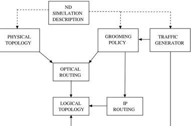
Fig. 1 represents the interaction between different GANCLES parts. A simulation starts after GANCLES has acquired the simulation experiment description in ND. The descrip-tion includes: (i) the network topology in terms of a weighted graph connecting USERS

and NODES through CHANNELS; (ii) the traffic relations between USERS and the sta-tistical characterization of sources; (iii) the selection of the routing, CAC and grooming algorithms adopted for the simulation run; (iv) a number of options concerning both the network operation and the simulation session management; (v) the performance indices to be measured.

When the simulation starts an optical-layer function independent from the selected RWA algorithm defines the set of available physical paths for each pair of OXCs/G-OXCs or-dering them according to some specific criterion. Only this set can be used by the routing algorithm, reducing the routing problem complexity.

Every time a new lightpath is added or removed from the network by the optical-layer, the data-layer (logical) topology is changed. As done at the optical-layer, also in this case the set of possible logical paths between each G-OXC (router) pair is computed following a user-specified criterion. This task is extremely critical, because path-computing is very

ROUTING IP OPTICAL ROUTING GROOMING POLICY LOGICAL TOPOLOGY GENERATOR TRAFFIC DESCRIPTION SIMULATION ND PHYSICAL TOPOLOGY

Figure 1: Logical interaction between different high-level modules in GANCLES, the management of the optical-layer is mediated by the grooming strategies and algorithms

time consuming, hence the path selection criterion must be carefully defined depending on the data-layer routing algorithm selected (e.g., only one path need to be computed if Fixed Shortest Path routing is used).

Notice that the overall setup (and performance) of IP over WDM networks is heavily influenced by technology constraints. We already mentioned opaque or transparent OXCs, but other constraints, such as simplex- of duplex-only lightpath management also come into play at the optical-layer. Similar constraints may arise if TE techniques are used at the data-layer. GANCLES allows the simulation of an arbitrary mix of these constraints. Each time a USER generates a connection request, the grooming algorithms decides whether: (i) route it over the current topology; or (ii) ask the optical-layer to open one or more lightpaths (thus modifying the logical topology) and then route the request at the data-layer. In the first case, a data-layer CAC algorithm (if any) is executed for each of the paths being considered by the data-layer routing algorithm; if no end-to-end path is found to route the incoming request in agreement with its QoS requirements, the request is dropped. In the second case, after the logical topology modification, the same data-layer routing and CAC are applied. As a general rule, in this case a connection can be refused only if the optical-layer was not able to modify the logical topology meeting the grooming algorithm requirements.

Modifying the logical topology, the question arises whether all the traffic is re-routed or if only new connections follow the new available routes. GANCLES presently assumes the second option, but its modification for re-routing is trivial.

When an active connection terminates, the corresponding resources in the logical topol-ogy are released. This operation can lead to the release of some lightpaths if they are not carrying traffic anymore. In this case, paths at the IP level need to be recalculated again over the new logical topology. The specific lightpath releasing criteria (e.g., a given time-lapse without traffic) can be specified by GANCLES user.

to keep each node informed of the network status. The control traffic is not considered in the performance measures.

3.2

Routing algorithms

In this section a short introduction to the routing algorithms available in GANCLES is given, at both data and optical level.

The routing options available in GANCLES differ from each other for the criteria they follow in order to select the paths that are to be tested by each traffic generator when a connection request is forwarded at run-time. When the simulation starts, the set of paths that connect every pair of nodes in the network must be known. So, after the network topology has been acquired by the simulator, a function not depending on the working routing algorithm takes care of defining the set of available paths for each pair of nodes. The paths are then ordered according to some specific criterion, and it is also possible to use some load-balancing algorithm, by setting specific parameters. The reader is referred to [18] for more details on this part.

Whatever criterion is used to order the paths, a primary path is always issued for each pair of nodes: it will be the first to be tested to route every connection between the involved nodes. All the other allowed paths are referred to as secondary paths.

3.2.1 Data-level routing

Several alternatives are available to route calls at data-level so as to take into account the dynamic load of the network. An important property of GANCLES is the possibility to simulate both source-based (e.g., MPLS-like) or hop-by-hop routing.

The following list enumerates the main routing algorithms implemented in GANCLES. The reader is referred to [18] for more details on this part and the relative references to the literature.

• Single Path Routing. With this algorithm, only the primary path between the nodes is considered to route the connection. If the CAC function issues a negative answer, even for a single link in the path, the connection is not accepted. With this al-gorithm, the resources employed to support each call are minimized, but it is not possible to adapt the routing strategy to the actual distribution of the traffic inside the network.

• Controlled Alternate Routing. With this algorithm, if there is no space for the call along the primary path, the secondary ones are investigated, according to the pri-orities assigned during the preliminary phase. A control mechanism is introduced in the investigation of a secondary path: the links belonging to this path have their

visible bandwidth reduced by an amount depending on the average load they are

destined to support when included in primary paths. Each link of the network is thus supplied with a secondary capacity (less than the original one) that has to be referred to each time the link is checked as part of a secondary path. This control

mechanism aims at forcing the connections to be preferably routed over the primary path, allowing them to get a secondary path only when the load currently carried therein is low.

• Uncontrolled Alternate Routing. This algorithm acts exactly as the previous one, but no capacity reductions affect the links included in the secondary paths. In this case the network is more exposed to the resource wasting that could derive from the spreading of connections over secondary paths. Nevertheless, under particular network configurations the uncontrolled alternate routing can be better than the previous one.

• Minimum Cost Routing. The algorithm selects the path π that minimizes the following quantity:

Cπ = aHπ + bDπ + c

1 minl∈π _NB_l+1l

where Hπ is the number of hops of the path, Dπ is the physical length of the path,

and 1

minl∈π Bl Nl+1

is the bandwidth available to a new call on the path’s bottleneck link. The coefficients a, b, c are user-specified parameters and can be used to tune the routing cost function.

• Load-Dependent Routing. This routing algorithm attempts to route calls over a path minimizing a cost function; however, if the bandwidth available on that path is less than a fraction of the bandwidth requested by the user, a shortest-path routing is preferred [23].

• Shortest-Widest Routing. The Shortest-Widest Routing algorithm first identifies the maximal-bandwidth path and breaks ties by choosing, among the paths with the maximum available bandwidth, the one with the minimum hop count

• Widest-Shortest Routing. The Widest-Shortest Routing algorithm first identifies the minimum-hop-count paths and breaks ties by choosing, among the paths with the minimum hop count, the one with the maximum available bandwidth. In prac-tice is a load balancing algorithm on shortest paths.

• Minimum Distance Routing. For each source-destination pair, the path π is cho-sen that minimizes the following quantity:

Cπ =

X

l∈π

1

bl

where bl is the max-min fair bandwidth that is available to a new connection over

link l belonging to path π.

The routing algorithms implemented in GANCLES are centralized with the single excep-tion of the Dynamic Least Congested Path routing algorithms, which are not considered here due to space reasons.

3.2.2 Optical-level routing

There are different static and dynamic algorithms implemented for the routing of ASON calls. In the following only single-path routing algorithms are described, but the tool al-lows to perform also protective routing, both with a dedicate or shared protection mech-anisms (see [19] for more details).

If we use opaque nodes, the wavelength continuity is necessary only in the transparent sections, i.e. the part of route connecting two opaque nodes. Allowing wavelength con-version in the opaque nodes implies that the wavelength assigned to the connection can be different in each transparent section.

In the current version of GANCLES, there are four main routing algorithms in the optical level:

• Fixed Shortest Path. This algorithm routes the call always on the dedicated pri-mary path between the endpoints. It is then a static routing algorithm.

• Shortest Lowest Path. This algorithm selects the path with the lowest available wavelength and then, if there are more possibilities, routes the call on the shortest among them. With Lowest wavelength we mean the wavelength with the smallest order number. Since in the different transparent section the lowest available wave-length can be different, we take the maximum of them to determine the metrics for the whole path.

• Shortest-Widest Path. This algorithm selects the path with the largest number of available channels and then, if there are more possibilities, routes the call on the shortest among them. Since in the different transparent section the number of available wavelengths can be different, we take the minimum of them to determine the metrics for the whole path.

• Alternate Shortest Path. This algorithm selects the shortest from those paths where there is at least one wavelength available.

Furthermore, two possible Wavelength Assignment (WA) algorithm are applied jointly with these routing algorithms:

• First-Fit WA: in this case, for each transparent section of the lightpath, the

low-est available wavelength is assigned. The objective here is to minimize the order

number of the highest used wavelength on the link.

• Random WA: in this case, for each transparent section of the lightpath, one of the available wavelengths is assigned by uniform probability. Obviously this WA scheme cannot be applied when using the Shortest Lowest Path routing algorithm.

3.3

Traffic Sources

Traffic sources play an important role during simulation experiments, since they generate connection requests and releases. Each connection request is associated with the identifier of the destination user, which is chosen accordingly to the traffic relations specified for the experiment. Connection request interarrival times and call durations are modelled as random variables with appropriate distributions. Two different kind of traffic sources are available in GANCLES, according to the level we are considering during simulations: the

data and the optical level.

3.3.1 Data-level users

At this level, there are five possible types of users:

• CBR users generate Constant Bit Rate connection request, i.e. the bit rate associ-ated to these connections are constant throughout their whole lifetime.

• ON-OFF CBR users, which model traffic sources that can either be transmitting at their maximum bit rate or be idle.

• Uniform Variable BR users, which model sources which continuosly change their bit rate between two fixed bounds.

• Video VBR users, whose bit rate can assume only three distinct values, according to a suitable probability distribution.

• Best-Effort users, that adapt their transmission rate to the current network conges-tion level as described below.

These source models can be grouped into classes, characterized by a different set of QoS parameters, and can be subjected to a specific CAC algorithm (see [18] for more details). In particular, the first four classes are inherited from the well-known ATM traffic models, and they correspond to bandwidth-guaranteed connections, while the last one model the IP best effort transfer capabilities, such as the traffic controlled by protocols with available rate feedback as TCP. The abstract model of this traffic is data flow with elastic bandwidth requirements.

Since GANCLES has been developed mainly to study the interaction between IP and the optical layer of a wavelength-routed network, a more detailed explanation of the elastic traffic features of BE users is fundamental to better understand this point. When elastic traffic is considered, no admission control is enforced, and no backpressure on traffic sources to reduce the average rate of connection generation is available, the network can become instable, as the number of flows within the networks can grow to infinity while their individual throughput goes to zero. To avoid this risk, and to build a more realistic scenario, a starvation threshold ths has been introduced, expressed as a fraction of the

peak bandwidth BM required by the flow. If at some time instant one or more flows

with the highest backlog is closed. Notice that if admission control is enforced, this simply means refusing the arriving flow instead of closing a flow as just described. The two actions are however not equivalent, because: i) the arriving flow may not be a starved one (e.g., has a smaller required BM); ii) blocking is not influenced by the flow dimension,

while the starvation is higher for larger flows; iii) starved flows waste network resources and may influence overall throughput, which is computed only on completed flows. Two different models of elastic traffic are available in the simulator. Both share the char-acteristic that a flow i arrives to the network with a backlog of data Di to transmit and

both include some form of elasticity, though very different one another.

The first model, called time-based (TB), assumes that the elasticity is taken into account only reducing the transfer rate when congestion arises. The flow duration τiis determined

when the flow arrives to the network, based on its backlog Di and its “requested

band-width” BM i(e.g., the peak negotiated rate, or the access link speed) τi = _BD_{M i}i . The effect

of congestion is just that the throughput of flows is reduced, but their closing time is not affected. A consequence of this behavior is that the data actually transferred by a flow

i is generally less than the “requested” amount Di. This model is very simple and does

not grab all the complexity of the closed-loop interaction between the sources and the network. It simply models the fact that the more congested is the network, the smaller is the throughput the flows get.

The second model, called data-based (DB), assumes instead an ideal max-min sharing of the resources within the network at any given instant. Flows still arrive to the network with a backlog Di, but the acceptance of a new flow will affect not only all the other

flows on the same path, but indeed all the flows in the network, since the max-min fair share is completely recomputed updating the estimated closing time of all the flows in the network. The same applies when flows close, freeing network resources. This model includes the most important feature of elastic traffic, which is the positive feedback on the flows duration. The more congested is the network, the longer the accepted flows remain in the network. Congestion spreads over time enhancing the possibility that still further flows arrive in the network worsening congestion. The DB model is clearly much more accurate, closely mimicking the behavior of an ideal congestion control scheme; however its complexity and computational burden are much larger, specially for high loads. 3.3.2 Optical-level users

Since GANCLES is based on the extension of an ASON based simulator [19], the traffic sources here considered are modelled according to the connection request generated into an ASON network. At this level, there are four possible types of users:

• Poisson ASON users, which defines a Poisson-like generator of ASON type calls; the generation of calls (lightpath requests) is characterized by an exponential inter-arrival time and an exponential holding time distribution.

• ON-OFF ASON users, which generates lightpath requests in on-off mode, i.e., they model traffic sources that can either be transmitting a connection between a source

and destination pair or be idle.

• Fixed ASON users, which model permanent and semi-permanent lightpath requests by generating calls that are never torn down.

• Pascal ASON users, which defines a Pascal-like generator of ASON type calls, then the generation of calls is characterized by an exponential interarrival time whose intensity depends on the network state. The distribution of the lightpath requests is typically more peaked than the Poisson one; these generators allow the modelling of bursty traffic.

3.4

Grooming algorithms

In GANCLES, when considering the interaction between the data and optical layers in an IP over WDM architecture, the basic assumption is that data-level users can trigger if needed the set-up of new lightpaths in the WDM layer. In particular, when a new connection request is generated from some of the data-level users described in Sect. 3.3.1, the decision of setting up a new lightpath or simply routing the incoming connection into the existing logical topology depends on the selected grooming policy. Obviously, the simulator allows the lightpath tear-down if no traffic is carried over it.

Before giving an overview of the implemented grooming policies, we first explain the interaction mechanisms between the data and the optical level allowed by the simulator. 3.4.1 Management of virtual links

When the two-level simulation is chosen, the data-level users have access only to the virtual topology, made of all the lightpaths installed in the optical network, while the physical links are completely hidden to them. Virtual links have the transmission capacity of one wavelength, which can be set in the network configuration file.

Since the lightpaths are set up through connection requests coming from the upper data-level, a new kind of lightpath traffic generator is introduced in this case, since most of the optical-level generators described in Sect. 3.3.2 do not fit well in this specific framework. Each time the establishment of a new virtual link is requested, a new lightpath is set-up as if it was generated by a Fixed ASON user, but in this case the connection can be torn down if it is not carrying traffic.

It is worth noticing that, even in the two-level simulation mode, GANCLES allows to share the optical resources among all the optical users described in Sect. 3.3.2. It is then possible to use this traffic as a background during the analysis of IP over WDM networks. When a lightpath needs to be released because it is not carrying traffic, the simulator gives the possibility of delayed closure using a timeout parameter, called optical closing

threshold τcl which can be specified by the user. When no traffic is carried over some

lightpath, the link is still open for the timeout period and gets closed only if its state does not change.

3.4.2 Current grooming policies

With grooming policies we indicate the decisions regarding possible changes of the cur-rent virtual topology each time a data-level connection request arrives or leaves the net-work.

When new virtual links need to be installed, two factors must be determined: how many of them must be set-up and between which nodes pairs. The grooming algorithm shall define both the factors according to the current load condition.

The decision to route the incoming requests over the existing virtual topology or to es-tablish new lightpaths to create more room for them can lead to different network perfor-mances. A general analysis of different “grooming policies” is carried out in [6] under the hypothesis of bandwidth-guaranteed traffic. When elastic traffic is considered, there is no obvious upper limit to the possible number of flows which is routed onto the exist-ing logical layer. In this case, the need for the establishment of new lightpaths must be introduced based on some suitable parameter. We introduce this parameter, called optical

opening threshold tho, as a threshold on the throughput that the incoming request would

achieve on the selected route, defined as a fraction of the peak rate BM irequired by each

flow.

Two solutions are implemented in the current version of simulator, both of them tries to open a new virtual link, if any. These two opposite policies have been often considered by different authors to perform comparisons with new grooming algorithms proposals or to study the impact of some specific network constraints, such as OXC node’s architecture. In this report, for the first time to the best of our knowledge, we consider them to study the impact of elastic traffic and analyze whether it affects them differently.

• Virtual-topology First (VirtFirst). This grooming algorithm aims to open new

op-tical lightpaths only if the current virtual topology does not have enough resources to carry the incoming request. First the connection is routed on the virtual topol-ogy and the bandwidth on the assigned route is analyzed. If there is no route at all between the source and destination nodes, a new virtual link is set up. Such conditions are easy to verify when bandwidth-guaranteed traffic such as CBR, ON-OFF CBR, Uniform VBR and Video VBR is generated at data-level traffic. When instead elastic traffic is considered, some new assumption needs to be introduced. If, once routed, the amount of bandwidth for the incoming elastic flow is less than

tho, a new lightpath is set-up between source and destination (if possible). If the

setup is successful the IP request is routed over it (it is a one hop route at the IP level) and a new virtual topology is computed at the IP level. The new topology does not affect already routed requests (i.e., no re-routing is considered), but will be used for routing all new requests. If the new lightpath cannot be set up, then the request is routed based on the current virtual topology. Note that if the source-destination pair is disconnected on the virtual topology and no new lightpath can be installed between them, the connection request is refused even if it is elastic. This behaviour can be considered pathological, since it means that a non-completely

connected was built on a completely connected physical topology; however, with grooming algorithms aggressive in using optical resources, we have observed it. Whenever a closing flow leaves a lightpath empty, the lightpath is closed too (after

τcl) and the virtual topology is re-computed.

• Optical-level First (OptFirst). Each time a new data-level request arrives in some

router, the G-OXC always attempts first to set up a new lightpath in the optical layer, in order to route the request over it. If no free wavelengths are available here, the IP router routes the incoming request over the current virtual topology. Indeed, a virtual topology is defined only when optical resources for the considered source-destination pair are exhausted. Note that if no new lightpath can be installed between the source-destination pair and they are disconnected also on the virtual topology, the connection request is refused even if it is elastic.

As in VirtFirst if a closing flow leaves a lightpath empty, the lightpath is closed after

τcl.

3.4.3 Important parameters with elastic traffic

As we shall discuss in Sect. 4, the phenomena involved in routing/grooming elastic traffic are rather complex, and often far from intuitive. As performance parameter we consider the following three (but more are available at both the IP and the optical level):

T : The average throughput per flow

T = 1 Nc Nc X i=1 ˆ Ti

where ˆTi is the average throughput of the flow i and Ncis the number of observed

flows (e.g., during a simulation). Notice that in a resource sharing environment this is not the average resource occupation divided by the number of flows, since flows have all the same weight, regardless of their dimension.

ps: The starvation probability. It is the probability that a flow is closed during its life

because it is not receiving service with acceptable quality. A flow i will close and drop the network if its instantaneous throughput Ti falls below a threshold ths

expressed as a fraction of the peak bandwidth request of the flow.

Nh: Average number of IP hops per flow.

4

The simulator at work

The aim of this section is to provide examples of the use of the simulation environment and of the results that can be obtained with it. We include here the simulation of a two-level IP over WDM network where data-two-level connection requests are elastic in nature,

G−OXC OXC 00 00 00 11 11 11 000 000 000 000 000 111 111 111 111 111 000 000 000 000 000 111 111 111 111 111 000 000 000 000 000 111 111 111 111 111 000 000 000 000 000 111 111 111 111 111 000 000 000 000 000 111 111 111 111 111 0000 0000 0000 0000 0000 0000 1111 1111 1111 1111 1111 1111 1 3 6 5 8 11 14 2 4 7 12 9 10 13

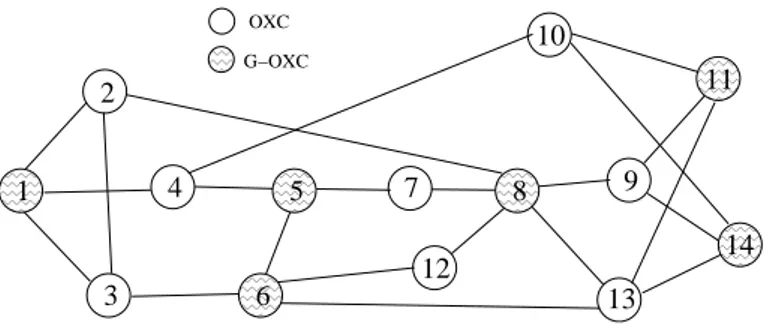
Figure 2: NSFNET topology

since this aspect is the most innovative from the simulation viewpoint. For examples of application of the tool in pure data or optical networks, we refer the reader to the list of publications reported in [18, 19].

In all the experiments, the network architecture considered is IP over WDM with dynamic optical routing, i.e., optical paths are opened on demand.

The optical level is based on Optical Crossconnects (OXC) interconnected by fiber links. Routing is fixed shortest-path with First-Fit wavelength assignment for the establishment of lightpaths. OXCs do not have wavelength conversion capabilities.

The IP level assumes traditional routers with dynamic shortest path routing based on the number of hops at the IP-level, so that an optical path is seen as a single hop regardless of the number of OXCs it crosses.

4.1

NSFNET

We present results obtained on the NSFNET network [22] shown in Fig. 2, which has 14 nodes and 21 fiber links. Each fiber carry up to 4 wavelengths, and only 6 nodes out of 14 have grooming capability, i.e., they are G-OXCs. Each wavelength has a capacity of 20 Gbps. A best-effort traffic source is connected to each G-OXC, opening flows with BM = 10 Gbps; each flow transfer data whose size is randomly chosen from an

exponential distribution with average 12.5 GBytes. A uniform traffic pattern is simulated, i.e., when a new traffic relation is generated, the source and destination are randomly chosen with the same probability; ths = 0.1 in all simulations and tho = thsfor the sake

of simplicity. All simulations are run until performance indices reach a 95% confidence level over a ±5% confidence interval around the point estimate.

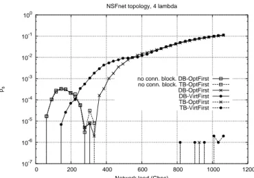
Fig. 3 presents a comparison of the average throughput T obtained modeling best-effort traffic relations using the TB approach (dotted lines) and the DB approach (solid lines) when the two grooming algorithms VirtFirst (round marks) and OptFirst (cross marks) are used. With the same graphic rules, Fig. 4 reports the starvation probability ps.

The difference in performance results of the two approaches is striking. Let’s consider first the OptFirst grooming policy. Both approaches show T starting from 10 Gbps when the offered load is low; however, they immediately diverge as the offered load increases. Indeed, the DB traffic model shows much faster decrease in T as soon as the offered load

2 3 4 5 6 7 8 9 10 0 200 400 600 800 1000 1200 T (Gbps) Network load (Gbps) NSFnet topology, 4 lambda

DB-OptFirst DB-VirtFirst TB-OptFirst TB-VirtFirst

Figure 3: Average throughput T for the DB and TB traffic models for the two grooming policies 10-7 10-6 10-5 10-4 10-3 10-2 10-1 100 0 200 400 600 800 1000 1200 ps Network load (Gbps) NSFnet topology, 4 lambda

no conn. block. DB-OptFirst no conn. block. TB-OptFirst DB-OptFirst DB-VirtFirst TB-OptFirst TB-VirtFirst

Figure 4: Starvation probability psfor the DB and TB traffic models for the two grooming algorithms

increases and this is due to the spreading of congestion over time with a sort of snow-ball effect. On the contrary, the TB traffic model shows a smoother decrease of the average bandwidth.

Analyzing the starvation probability in Fig. 4 adds more insight. When the traffic is very low (below 350 Gbit/s) both traffic models show the same, very strange behavior: the starvation increases and then decreases sharply. This form of blocking is independent of the traffic model and it is due to a very aggressive and dynamic use of optical resources that sometimes leads to have no connectivity at the IP level, i.e., a flow request arrive and there is no possible path, neither optical, nor through multiple IP hop, between the source and the destination. When the load increases, however, lightpaths become more stable (because there is always traffic keeping lightpaths open) and the probability that the virtual topology is not completely connected becomes negligible. To highlight the difference of this phenomenon from the real starvation, in Fig. 4 the curves relative to it are plotted with square marks. When the load increases further, the two traffic models behavior diverges: the TB model show no starvation at all, apart from points at very high loads, which show a blocking probability around 10−6, while the DB model show a starvation probability increasing steadily. This difference in the starvation behavior enhance the differences in T , since aborting flows cause a waste of bandwidth.

When considering the VirtFirst grooming policy instead, the behaviour of both traffic model is different from the previous one. Both DB and TB T decrease sharply even when the offered load is low, due to the conservative policy of VirtFirst. In fact, VirtFirst sets up the minimum number of lightpaths in order to guarantee the minimum network con-nectivity, and keeps this configuration unchanged until some flow crosses the starvation threshold ths. Only in this case VirtFirst increases the resources at IP level by setting

up new lightpaths. In particular, the T for DB traffic relations decreases very rapidly, causing an earlier set-up of new lightpaths compared to TB traffic. This lead the DB traffic throughput T to “bounce” taking advantage of the higher number of lightpaths in the network, at a load much smaller than for the TB model, that starts increasing again at higher loads. Obviously, both models would show another (and definitive) decrease in

T for higher loads, not simulated here. It is interesting to notice that the starvation rate

(see Fig. 4) for the TB model is in this case always zero (apart from a single point around load 900 Gbit/s), while the starvation rate of the DB model increases steadily and shows a behavior similar to the DB model in the OptFirst case.

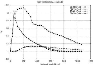
Fig. 5 reports the average number of IP hops per flow Nh. As expected the OptFirst policy

keeps this parameter very close to one. The VirtFirst instead show a sharp increase for low loads due to the fact that at very low loads the probability that a flow arrives and find the virtual, IP topology already connecting the source and destination is very low, thus a new lightpath is always opened also with VirtFirst policy. As the load increase, this parameter converges to one also in the VirtFirst case, since the number of wavelength per link considered allows a complete optical mesh connecting every G-OXC. Clearly this would be different in different topologies or if a smaller number of wavelengths per link were considered.

0.8 1 1.2 1.4 1.6 1.8 2 2.2 0 200 400 600 800 1000 1200 Nh Network load (Gbps) NSFnet topology, 4 lambda

DB-OptFirst DB-VirtFirst TB-OptFirst TB-VirtFirst

Figure 5: Average number of hops Nhat the IP level.

5

Conclusions

The rationale, the capabilities and the implementation of GANCLES, a simulation envi-ronment for the analysis of realistic IP over WDM networks were described. The simula-tion environment is based on extensions of the connecsimula-tion level simulator ANCLES [18], which regards the introduction of best-effort, elastic traffic as described in [12] and some related to the introduction of optical routing capabilities [19].

The development of an integrated set of functionalities at different levels, data (IP or ATM), optical (WDM) and data-over-optical, permits a unique and consistent description of optical networks.

An example of the use of GANCLES for the analysis of some network configuration provided evidence of the effectiveness of the proposed approach.

This technical report will evolve with new versions as GANCLES evolves, new capabili-ties are added to it and new grooming algorithms are defined and implemented.

References

[1] N. Ghani, S. Dixit, T.S. Wang, “On IP-WDM Integration: A Retrospective,” IEEE

Communications Magazine, 41(9):42–45, Sept. 2003.

[2] P. Molinero-Fernandez, N. McKeown, H. Zhang, “Is IP going to take over the world (of communications)?,” ACM SIGCOMM Computer Communications

Re-view, 33(1):113–119, Jan. 2003.

[3] M. Ajmone Marsan, N. Golmie, D. Montgomery, R. Sharma Eds., “Special issue: Simulation, CAD, and Measurement of Optical Networks,” SPIE Optical Network

[4] R. Dutta, G.N. Rouskas, “Traffic grooming in WDM networks: past and future,”

IEEE Network Magazine, 16(6):46–56, Nov./Dec. 2002.

[5] X. Zhang, C. Qiao, “An Effective and Comprehensive Approach to Traffic Grooming and Wavelength Assignment in SONET/WDM Rings,” IEEE/ACM Transactions on

Networking, 8(5):608–617, Oct. 2000.

[6] H. Zhu, H. Zang, K. Zhu, B. Mukherjee, “A novel generic graph model for traffic grooming in heterogeneous WDM mesh networks,” IEEE/ACM Transactions on

Networking, 11(2):285–299, Apr. 2003.

[7] K. Zhu, B. Mukherjee, “Traffic grooming in an optical WDM mesh network,” IEEE

Journal on Selected Areas in Communications, 20(1):122–133, Jan. 2003.

[8] M. Brunato, R. Battiti, “A multistart randomized greedy algorithm for traffic groom-ing on mesh logical topologies,” In Proc. of the 6th IFIP ONDM, Torino, Italy, Feb. 2002.

[9] M. Kodialam, T.V. Lakshman, “Integrated Dynamic IP and Wavelength Routing in IP over WDM Networks,” In Proc. of INFOCOM 2001, pp. 358–366, Anchorage, AK, USA, Apr. 22–26 2001.

[10] X. Niu, W.D. Zhong, G. Shen, T.H. Cheng, “Connection Establishment of Label Switched Paths in IP/MPLS over Optical Networks,” Photonic Network

Commu-nications, 6:33–41, July 2003.

[11] R. Srinivasan, A.K. Somani, “Dynamic Routing in WDM Grooming Networks,”

Photonic Network Communications, 5:123–135, Mar. 2003.

[12] C. Casetti, R. Lo Cigno, M. Mellia, M. Munaf`o, Z. Zs´oka “A Realistic Model to Evaluate Routing Algorithms in the Internet,” In Proc. IEEE Globecom 2001, San Antonio, Texas, USA, pp. 1882–85, Nov. 25–29, 2001.

[13] OPNET - OPNET Technologies.

URL: http://www.opnet.com

[14] M. Ajmone Marsan, A. Bianco, C. Casetti, C.F. Casserini, A. Francini, R. Lo Cigno, M. Munaf`o, “An integrated simulation environment for the analysis of ATM net-works at multiple scale times,” Computer Netnet-works and ISDN, 29(17-18):2165– 2185, February 1998.

[15] A. Francini, “Statistics User Manual, Politecnico di Torino,” March 1994,

URL: ftp://ftp.tlc.polito.it/pub/class/statistics.ps

[16] A. Banerjee, J. Drake, J.P. Lang, B. Turner, K. Kompella, Y. Rekhter, “Generalized Multiprotocol Label Switching: an Overview of Routing and Management Enhance-ments,” IEEE Communications Magazine, 39(1):144–150, Jan. 2001.

[17] GANCLES - Grooming Ancles.

URL: http://ardent.unitn.it/gancles

[18] ANCLES - A Network Call-Level Simulator.

URL: http://www.tlc-networks.polito.it/ancles

[19] ASONCLES - ASOn Network Call-Level Simulator.

URL: http://www.hit.bme.hu/ zsoka/asoncles

[20] K. Pawlikowski, “Steady-state simulation of queueing processes: a survey of prob-lems and solutions,” ACM Computer Surveys, 22(2):123-170, June 1990.

[21] A.A. Kherani, A. Kumar, “Stochastic Models for Throughput Analisys of Randomly Arriving Elastic Flows in the Internet,” In Proc. IEEE Infocom 2002, Nwe York, NY, USA, June 23–27, 2002

[22] O. Crochat, J. Boudec, “Design protection for WDM optical networks,” IEEE

Jour-nal on Selected Areas in Communications, 16(7):1158–1165, Sep. 1998.

[23] C.Casetti, G.Favalessa, M.Mellia, M.Munaf`o, An Adaptive Routing Algorithm

for Best-effort Traffic in Integrated-Services Packet Networks, IEE ITC’99,