Università Politecnica delle Marche
Scuola di Dottorato di Ricerca in Scienze dell’Ingegneria Curriculum in Ingegneria Civile, Edile e Architettura
XV edition - New series
---
Multiscale Rheological and Mechanical
characterization of Cold Mixtures
Ph.D. Dissertation of:
Carlotta Godenzoni
Advisor:
Prof. Maurizio Bocci
Co-Advisor:
Curriculum Supervisor:
Dr. Ph. D. Andrea Graziani Prof. Stefano Lenci
Pavement-scale
M
Ixt
ure
-sca
le
M
astic
-sca
le
Mortar-scale
Università Politecnica delle Marche
Scuola di Dottorato di Ricerca in Scienze dell’Ingegneria Curriculum in Ingegneria Civile, Edile e Architettura
---
Multiscale Rheological and Mechanical
characterization of Cold Mixtures
Ph.D. Dissertation of:
Carlotta Godenzoni
Advisor:
Prof. Maurizio Bocci
Co-Advisor:
Dr. Ph. D. Andrea Graziani
Curriculum Supervisor:
Prof. Stefano Lenci
Università Politecnica delle Marche
Dipartimento di Ingegneria Civile, Edile e Architettura
To my Family
“…Experience is not what happens to you...
it’s what you do with what happens to you…”
i
Acknowledgements
Desidero ricordare tutti coloro che mi hanno sostenuto durante questi tre anni di dottorato: a loro va la mia gratitudine, anche se a me spetta la responsabilità per ogni imperfezione contenuta in questa tesi.
Ringrazio anzitutto il Professor Maurizio Bocci, Relatore, e l'Ing. Andrea Graziani, Co-relatore della presente tesi di dottorato: senza il loro supporto e la loro guida sapiente questa tesi non esisterebbe. Proseguo con il Professor Francesco Canestrari, professionista instancabile della ricerca da cui si può trarre solo esempio, fuori e dentro l'ambiente accademico. Un ringraziamento particolare lo voglio rivolgere al Professor Daniel Perraton e al Dottor Emmanuel Chailleux responsabili scientifici delle mie esperienze di ricerca internazionali, rispettivamente presso l’”École de technologie supérieure” (Montréal, Canada) e l’”Institut français des sciences et technologies des transports, de l'aménagement et des réseaux” (Nantes, Francia).
Un grazie di cuore lo dedico ai colleghi del Dipartimento DICEA-Area Strade, ricercatori, tecnici e dottorandi che prima di essere compagni di lavoro sono stati compagni di vita ma soprattutto amiche inestimabili e insostituibili. Grazie Arianna, Francesca e Giorgia! Vorrei infine ringraziare le persone a me più care: i miei genitori Mauro e Rosanna che mi hanno supportato ma soprattutto sopportato in questo lungo percorso, mia nonna Maria sempre al mio fianco e infine il mio compagno e collega Emiliano.
Ancona, 10 Febbraio 2017
Abstract
Nowadays, the growing social and political awareness about environmental issues is moving towards the development of low-energy and low-emission technologies. In this context, cold technologies as cold mixtures may represent a valid alternative to traditional hot mix asphalt for road pavements. Cold mixture combines both economic and environmental benefits related to the reduction of energy necessary for heating both bitumen and aggregates. Moreover, when cold mixtures are adopted for pavement recycling, the consumption of virgin aggregate can be significantly reduced.
In the past, the use of cold mixture for structural layers has attracted relatively little attention largely because of problems related to the time required for full strength to be achieved after paving and its susceptibility to early life damage by rainfall.
Currently, the profound lack of technical guidelines and adequate standardized procedures, forces technicians and professionals to refer exclusively to previous experiences.
The PhD research aimed at scientifically verifying advantages and disadvantages of cold mixtures. To this aim an extensive experimental study was carried out involving advanced characterizations in order to identify the physical, mechanical and rheological behavior of cold mixtures.
Besides the traditional laboratory investigations, an original research methodology based on the multiscale analysis was applied. In fact, cold mixture can be considered as an evolutive material because its physical state evolves over time according to moisture loss. In this context, the characterization of cold mixture should be developed at different time during the in-service life of the material (time-scale) and at different level of investigation (size-scale). Optimum correlation was found between the results collected from different levels of investigation (size and time-scales); hence demonstrating the scientific validity of the adopted research approach. A detailed description of specific results carried out in these investigations can be found in the “Summary” section of each chapter.
Based on the overall findings, no elements discourage the use of cold mixture as support layers for pavement structure. Therefore, materials should be properly designed in terms of aggregate blend, water content and binding agents (type and dosage).
According to this observation, it can be concluded that using specific precautions, the adoption of cold mixture may contribute to improve and preserve the performance of road pavements.
Sommario
Oggigiorno, la crescente consapevolezza sociale e politica riguardante le questioni ambientali si sta orientando verso lo sviluppo di tecnologie a basso consumo e basse emissioni. In questo contesto, le tecnologie a freddo come le miscele bituminose a freddo possono rappresentare una valida alternativa ai tradizionali conglomerati bituminosi a caldo, per le pavimentazioni stradali. L’adozione di miscele bituminose a freddo combina benefici sia economici che ambientali legati alla riduzione dell'energia necessaria per il riscaldamento sia il bitume che di aggregati. Inoltre, quando questi materiali vengono utilizzati per il riciclaggio di pavimentazioni stradali ammalorate, il consumo di aggregati vergini può essere considerevolmente ridotto.
In passato, l'uso di miscele bituminose a freddo per strati di pavimentazione ha attirato relativamente poca attenzione soprattutto a causa dei problemi legati al tempo richiesto per il completo sviluppo di resistenza e la sua suscettibilità all’infiltrazione di acque meteoriche, nei primi mesi di vita.
Attualmente, la profonda mancanza di linee guida e di adeguate procedure standardizzate, costringe i tecnici e professionisti che voglio confrontarsi con l’utilizzo di queste nuove tecnologie, a riferirsi esclusivamente a esperienze precedenti.
Il presente dottorato di ricerca è volto a verificare scientificamente i vantaggi e gli svantaggi dell’adozione di miscele bituminose a freddo. A tale scopo, è stato condotto un vasto studio sperimentale servendosi di caratterizzazioni avanzate per identificare il comportamento fisico, meccanico e reologico di questo materiale.
Oltre alle tradizionali indagini di laboratorio, è stata applicata una metodologia di ricerca originale basata sull'analisi multiscala. Infatti, la miscela bituminosa a freddo può essere considerata come un materiale evolutivo poiché il suo stato fisico evolve nel tempo a causa della continua perdita di umidità. In questo contesto, la caratterizzazione delle miscele bituminose a freddo deve essere sviluppata su scale temporali differenti durante la vita in servizio del materiale e a diversi livelli di indagine (scala dimensionale).
I risultati raccolti ai diversi livelli di indagine (scale temporali e dimensionali) hanno mostrato una correlazione ottimale tra loro; a dimostrazione del fatto che il metodo di ricerca adottato può ritenersi scientificamente valido. Una descrizione dettagliata dei risultati ottenuti in queste indagini sperimentali sono stati riportati nella sezione "Sommario" di ciascun capitolo.
Sulla base dei risultati complessivamente ottenuti, nessun elemento scoraggia l'uso delle miscele bituminose a freddo come strati di supporto per la sovrastruttura stradale. Ad ogni modo, i materiali impiegati devono essere adeguatamente progettati in termini di assortimento granulometrico, contenuto d'acqua e di leganti (tipo e dosaggio).
In conclusione si può affermare che, seguendo particolari accorgimenti, l'adozione di miscele bituminose a freddo può contribuire a migliorare e preservare le prestazioni delle pavimentazioni stradali.
Contents
Acknowledgements………...i
Abstract………ii
Sommario………iii
Contents………..iv
List of Figures………..x
List of Tables………xix
List of Standard Specifications………..xxii
Introduction
………..3
1. Background and problem statement……….5
2. Lite
rature review………...11
2.1 Backg
round………..……...11
2.2 Recycling of bituminous
pavements………....13
2.3 Major issues related to
cold recycling technique………...………..14
2.4 State of the art in Europe………..…19
2.4.1 European projects
……….…...20
2.5 State of the art in Southern Africa..………..…22
2.6
State of the art in Northern America..……….23
2.7 Cold mixtures……….……….24
2.7
.1 Cement treated materials………..26
2.7
.2 Bitumen stabilized materials……….27
2.7.3 Cement-
bitumen treated materials………....29
2.8 Constituents of cold
mixtures………..………32
2.8
.1 Aggregates (virgin or recycled) ………...32
2.8
.2 Cement………....……….36
2.8
.3 Bitumen emulsion ………....37
2.8
.4 Foamed bitumen ………..46
2.8
.5 Fluid content………...52
2.9 Compac
tion………...56
2.10 Volumetric properties of cold
mixtures………..………...56
2.10.1 CM
– foam….………...………...57
2.10.2 CM
– emulsion…………...………59
2.11 The evolutive behavior: key feature of C
Ms………….…………...64
2.12
Viscoelastic properties………..66
2.12
.1 Different test protocols………...68
3. Research description and objectives………71
3.1 Methodological approach………....72
3.2 Outline of the dissertation………...…75
Part 1: Pavement-scale analysis: Cold mixtures for
subbase layers...
……….…79
4. Introduction………...81
5. Evaluation of pavement performance using non-destructive
testing and laboratory validation……….84
5.1 Field equipmen
t: falling weight deflectometer………...85
5.1.1 General description………...85
5.1.2 Load pulse………86
5.1.2 Deflection sensors………....87
5.1.3 Dynamic analysis of FWD data………....88
5.2 Laboratory equipm
ent, test methods and data analysis…………...92
5.2.1 Nottingham Asphalt Tester………...92
5.2.2 Cyclic uniaxial compression tests……….93
6. Experimental pavement section: SS38 Highway
Merano-Bolzano………...97
6.1 General overview………....97
6.2 Pavement structure………...99
6.3 Materia
ls………...100
6.4 Construction sequence………...102
6.5 Testing program
……….105
6.5.1 Laboratory testing………...105
6.5.2 FWD
testing………...106
6.6 Experimental findings and analysis………..……….107
6.6.1 Laboratory testing………...107
6.6.2 FWD testing………...113
6.7
Pavement performance………118
6.8
Summary……….121
7. Evaluation of in-situ curing process using Time Domain
Reflectometer probes and laboratory validation……….….122
7.1 Field equipment……….123
7.
1.1 Time domain reflectometer……….123
7.1.2 Temperature probes………....125
7.1.3 Data Acquisition Hardware………..………..125
7.1.4 Earth pressure cell………...…………...126
7.1.5 Asphalt strain gauges………...126
7.1.6 Sign
al conditioning and data acquisition system…………....127
7.2 Laboratory equipment, test methods and data analysis……….…128
7.2.1 Specimens compaction: laboratory procedure using Shear
Gyratory Compactor………....128
7.2.2 Indirect Tensile Stiffn
ess Modulus……….130
7.2.3 Indirect Tensile Test………...131
7.2.4 Curing process: modelling………..132
8. Instrumented pavement section: A14 Motorway
Bologna-Taranto……….136
8.1 Project description………136
8.1.1 Objective and methodology………...137
8.2 Experimental program………...138
8.2.2 Mixtures……….139
8.2.3 TDR probes: laboratory calibration………...139
8.2.4
On-site
construction
operations
and
instruments
installation………...143
8.2.5 Laboratory procedure for specimens production…………...148
8.2.6 Curing………...148
8.2.7 Testing methods………...…..149
8.3 Experimental findings:
analysis and modelling………...149
8.3.1 Volumetric properties
……….149
8.3.2 Evolution of material properties and model fitting
……..151
8.3.3 Relation between moisture loss and mechanical properties
……….158
8.3.4 Re
lation between mechanical properties………...160
8.4 Summ
ary………...161
Part 2: Mixture-scale analysis: Laboratory characterization of
Cold mixtures………..……….165
9. Introduction……….167
10. Curing process:
analysis and modelling for CBTM…....169
10.1 Experimental investigation………..169
10.1.1 Materials………...169
10.1.2 CBTM specimens production………...170
10.1.3 Water content optimization………...171
10.1.4
Test program and curing procedure………..173
10.1.5 Modelling of curing effects………...174
10.2 Experimental findings……….176
10.2.1 Volumetric properties of the tested specimens………..176
10.2.2 Evolution of material properties………...178
10.2.3 Relation between moisture loss and mechanical properties
……….185
10.2.4 Relation between mechanical properties………..187
10.3 Summary………...189
11. Influence of reclaimed asphalt on viscoelastic properties of
cement-
bitumen treated materials……….190
11.1 Experimental program……….190
11.1.1 Materials and mixtures……….190
11.1.2 Composition and volumetric properties of CBTM
mixtures………...194
11.1.3 CBTM-BE mixture: specimens preparation and water
optimization……….…...198
11.1.4 CBTM-FB mixture: mix-
design procedure………..199
11.2 Complex modulus testing procedure………...202
11.2.1 CBTM-
BE specimens………...202
11.2.2 CBTM-
FB specimens………...203
11.3 Experimental findings: CBTM-
BE……….204
11.3.1 Volumetric properties and optimal water content…………204
11.3.2 Complex modulus results……….207
11.4 Experimental findings: CBTM-
FB……….210
11.4.1 Volumetric properties and optimum foamed bitumen
content……….……210
11.4.2 Complex modulus results………...…..213
11.4.3 Advanced rheological modelling………...218
11.5 Summary and comparison………...222
11.5.1 CBTM-
BE mixtures………...222
11.5.2 CBTM-
FB mixtures………...223
11.5.3 CBTM-BE vs CBTM-
FB mixtures………...223
12. Three-dimensional linear viscoelastic response of cold
recycled mixtures
………226
12.1 Ove
rview……….226
12.2 Measurement of Poisson’s ratio of bituminous materials…………...227
12.3 Experimental program……….229
12.3.1 Materials and mixtures……….229
12.3.2 Sample preparation………...229
12.3.3 Test setu
p and data acquisition……….230
12.3.4 Laboratory testing: test program and analysis of time
histories……….…..232
12.4 Experimental findings………...235
12.4.1 Analysis of complex Young’s modulus………...235
12.4.2 Anal
ysis of complex Poisson’s ratio………237
Part 3: Mortar-scale analysis: Laboratory characterization of
Cold bituminous mortars……….……...241
1
3. Introduction………...243
13.1 General overview
………...243
14. Laboratory characterization of Cold bituminous mortar
………...245
14.1 Experimental program………245
14.1.1 Preliminary phase1: mixing design water content, W
des……….246
14.1.2 Preliminary phase2: mixing design compaction energy,
N
des………..247
14.1.3 Mechanical testing………...247
14.2 Materials and mortars
……….248
14.2.1 Samples production and curing procedure………...251
14.3 Labora
tory equipment, test methods and data analysis………...251
14.3.1 Indirect tensile stiffness modulus………..251
14.3.2 Indirect tensile strength……….251
14.3.3 Semi Circular Bending……….255
14.3.4 Scanning electron microscope………...258
14.4 Experimental findings: preliminary phase………..261
14.4.1 Mixing design water content………262
14.4.2 Mixing design compaction energy………...266
14.5 Experimental findings: mechanical testing……….269
14.5.1 Indi
rect tensile stiffness modulus……….269
14.5.2 Indirect tensile strength………270
14.5.3 Semi-
circular bending test………....275
14.5.4 Modelling of curing process……….276
14.5.5
Microstructure
observation
by
scanning
electron
mi
croscope……….……….278
14.6 Summary………..……...281
Part 4: Mastic-scale analysis: Rheological characterization of
Cold bituminous mastics……….285
15. Introduction………...287
15.1 General overview………....287
16. Rheological characterization of Cold bituminous mastics
………...290
16.1 Experimental program……….290
16.2 Materials and mastics………...291
16.2.1 Production protocol of mastic sampl
es……….293
16.3 Laboratory equipment, test methods and data analysis………...295
16.3.1 Kinexus Pro+ dynamic shear rheometer………...295
16.3.2 Metravib DMA+450………...298
16.3.3
Rheological
data
analysis:
DSR
and
Metravib
measurement
s………..………....300
16.4 Experimental findings: complex shear modulus G
*………….……..304
16.4.1 Effect of curing process………..……..304
16.4.2 Effect of volumetric concentration ratio………...309
16.4.3 Effect of mineral addition type………...310
16.5 Experimental findings: Complex Young’s modulus E*………..311
16.5.1 Effect of curing process………....311
16.5.2 Effect of volumetric concentration ratio………...315
16.5.3 Effect of mineral addition type……….316
16.6 Rheologica
l modeling……….317
16.7 Summary………...324
Summary of the overall experimental study……….327
17. Concluding remarks………..329
3-
years Ph.D. publications………..332
List of Figure
Figure 1. 1 Three Pillars of Sustainability. ... 6
Figure 1. 2 Generic life cycle of a production system for LCA [Kendall, 2012]. ... 8
Figure 2. 1 Pavement maintenance and rehabilitation. ... 12
Figure 2. 2 Pavement condition and type of in-place recycling method [Fisher, 2008]. .... 14
Figure 2. 3 Cold recycling process: a) in-plant and b) in-place. ... 15
Figure 2. 4 Typical equipment used for CIR recycling and FDR reclamation trains [Thompson et al., 2009]. ... 19
Figure 2. 5 Classification of bituminous mixtures in terms of aggregate mixing temperature and energy consumption for heating, Reference material at 20 °C and varying moisture content (mc). ... 25
Figure 2. 6 Conceptual composition of pavement mixtures [Asphalt Academy, 2009; Grilli et al., 2012]. ... 26
Figure 2. 7 BSM structure: with bitumen emulsion, BSM-emulsion; with foamed bitumen BSM-foam. ... 28
Figure 2. 8 Cement-bitumen treated material (CBTM) composed by: VA, RA, cement, bitumen emulsion and voids. ... 30
Figure 2. 9 Example of petrographic examination result of a sand. particle dimensions less than 0.075 mm under plane polarized light. ... 32
Figure 2. 10 Reclaimed asphalt (RA). ... 34
Figure 2. 11 Semi-brittle behavior of material stabilized with cementitious agents. ... 37
Figure 2. 12 Types of emulsions: a) O/W emulsion; b) W/O emulsion and c) multiple W/O/W emulsion. ... 38
Figure 2. 13 Typical particle size distribution of bitumen emulsion droplets. ... 38
Figure 2. 14 Stages in the breakdown of emulsions. ... 39
Figure 2. 15 Manufacture of bitumen emulsion: in batch and inline emulsion production. 40 Figure 2. 16 Diagram of emulsification process. ... 41
Figure 2. 17 Cationic emulsifier molecule. ... 41
Figure 2. 18 Typical DLVO interaction between two bitumen droplets and its two main electrostatic and Van der Waals components: interaction energy (in units of thermal energy kT) versus interparticle distance. ... 43
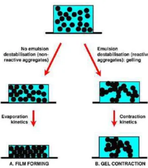
Figure 2. 19 The two possible breaking scenarios for the bitumen emulsion: a) film forming and b) gel contraction. ... 44
Figure 2. 20 Production of foamed bitumen in an expansion chamber. ... 48
Figure 2. 21 Generalized foam with non-spherical bubbles [Schramm, 1994]. ... 48
Figure 2. 22 Continuously and non-continuously bounds for bitumen emulsion and foamed bitumen, respectively. ... 48
Figure 2. 23 Foam characteristics for typical bitumen. ... 50
Figure 2. 24 Foam decay curve for selected bitumen with 2% of foamant water. ... 50
Figure 2. 25. Determining the optimum foamant water content (OFWC). ... 52
Figure 2. 26 Proctor compaction test results [Grilli et al., 2012]. ... 55
Figure 2. 27 Volumetric of voids in filler/bitumen mastic for foamed bitumen [Cooley et al., 1998]. ... 58
Figure 2. 28 Volumetric composition of a CM produced with foamed bitumen, considering
the influence of fluid content on VMA for a specific compaction level. ... 59
Figure 2. 29 Typical component materials for CBTM before emulsion breaking [Grilli et al., 2012]. ... 60
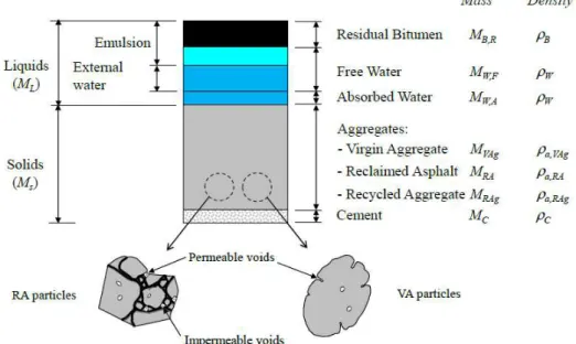
Figure 2. 30 Volumetric analysis of CM produced with bitumen emulsion [Grilli et al., 2012]. ... 61
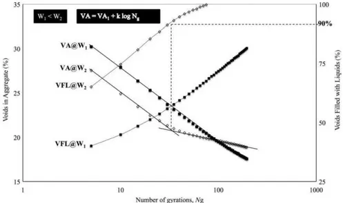
Figure 2. 31 Evolution of VA and VFL parameters as a function of SGC gyrations, at different water content W1<W2 [Grilli et al., 2012]. ... 63
Figure 2. 32 Concept of Curing and Influence on Mix Stiffness for BSMs [Asphalt Academy, 2009]. ... 64
Figure 2. 33 Typical mix behavior domains [Di Benedetto and De La Roche, 1998; Di Benedetto et al., 2001]. ... 67
Figure 2. 34 Sinusoidal Signals solved in Complex Plane... 68
Figure 2. 35 Methods of applying sinusoidal loading. ... 68
Figure 2. 36 SST shear and axial dynamic modulus testing. ... 70
Figure 3. 1 Multiscale dependencies of bituminous mixtures. ... 73
Figure 3. 2 Multiscale composition of cold mixture. ... 74
Figure 3. 3 Evolutive behavior of cold mixtures. ... 75
Figure 3. 4 Experimental activities set up. ... 75
Figure 5. 1 Schematic diagram of FWD equipment. ... 86
Figure 5. 2 Scheme of deflection basin. ... 86
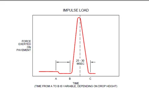
Figure 5. 3 Time to Peak Load for Impulse-Based on FWD equipment. ... 87
Figure 5. 4 Deflection sensor: geophone type... 88
Figure 5. 5 Deflection sensor: seismometer type. ... 88
Figure 5. 6 Comparison of measured and calculated deflection basins. ... 89
Figure 5. 7 BAKFAA Software. ... 91
Figure 5. 8 Nottingham Asphalt Tester (NAT) ... 93
Figure 5. 9 Cyclic uniaxial compression tests ... 94
Figure 5. 10 Time-Temperature Superposition principle: schematic representation. ... 95
Figure 5. 11 Huet-Sayegh (H-S) rheological model representation (Cole-Cole plane) [Di Benedetto et al., 2011]. ... 96
Figure 6. 1 Location of the experimental pavement section (source: Google Streetview). 97 Figure 6. 2 Maximum, average and minimum annual temperatures, from 2007 to 2015. .. 98
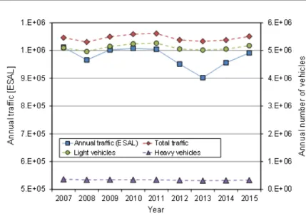
Figure 6. 3 Traffic data SS38 highway, recorded from 2007 to 2015: annual number of vehicles (light, heavy and total) and annual traffic (ESALs). ... 99
Figure 6. 4 Configuration of the experimental pavement section. ... 100
Figure 6. 5 Grading curves of RA, RAg and the adopted aggregates blend. ... 101
Figure 6. 6 Construction sequence adopted for the experimental pavement section: a) 1st milling; b) 2nd milling; c) 3rd milling; d) RA replacing e) 1st pass of the recycler; f) Spreading of cement; g) 2nd pass of the recycler for the subbase stabilization; h) Paving with HMA. ... 104
Figure 6. 7 Photos taken during the construction of the experimental pavement section: a)
emulsion; c) Subbase compaction by means of pneumatic tire roller; d) Laydown of the
HMA base layer. ... 105
Figure 6. 8 Cored samples from the experimental pavement section. ... 106
Figure 6. 9 Photos taken during the FWD measurements performed on both the right and the left wheelpath. ... 107
Figure 6. 10 Isothermal curves of the stiffness modulus (E0) measured on: a) HMA1, b) FB2, c) BE3 and d) CTM1. ... 109
Figure 6. 11 Master curves of the stiffness modulus E0 at 20 °C: a) HMA specimens, b) FB specimens, c) BE specimens and d) CTM specimens. ... 111
Figure 6. 12 Isochronous master curves at the reference frequency of 10 Hz for HMA, CBTM-FB, CBTM-BE and CTM... 112
Figure 6. 13 Central deflections profiles D0 measured in June 2007, one month after the rehabilitation operations, and in December 2007, i.e. after 6 months. ... 115
Figure 6. 14 FWD central deflections recorded during 8 years of FWD inspections, from June 2007 to 2015. ... 115
Figure 6. 15 BDI calculated on and for 8 years of FWD inspections. ... 116
Figure 6. 16 The mechanical performance of HMA, CBTM-FB, CBTM-BE and CTM during a period of 8 years in terms of stiffness modulus E0, normalized with respect to its initial value. ... 119
Figure 6. 17 Isochronous master curves at 10 Hz and back-calculated moduli for a) HMA, b) CBTM-FB, c) CBTM-BE and d) CTM. ... 121
Figure 7. 1 TDR probe Mod. CS616. ... 125
Figure 7. 2 Thermistor Mod.108. ... 126
Figure 7. 3 Configuration for measuring water content and temperature data, Campbell Scientific. ... 127
Figure 7. 4 Geokon Earth Pressure Cell... 127
Figure 7. 5 CTL Asphalt Strain Gauge. ... 128
Figure 7. 6 Data acquisition system layout. ... 129
Figure 7. 7 Comparison between SGC laboratory and field compaction. ... 130
Figure 7. 8 Form of load pulse, showing the rise-time and the peak (EN 12697-26). ... 132
Figure 7. 9 Michaelis-Menten model: an example with yA= 1 and Kc = 7 days. ... 134
Figure 7. 10 Relationship between curing rates of DW and ITS and curvature of ITS = ITS (DW). ... 136
Figure 8. 1 Location of the test section (source: Google Streetview). ... 137
Figure 8. 2 Experimental pavement section: a) plain and b) cross section view. ... 138
Figure 8. 3 Gradation of aggregate blend (EN 933-2) and specification limits for A14 motorway construction. ... 140
Figure 8. 4 Calibration of the CS616 moisture probes: a) PVC tube; b) and C) installation of TDR probe d) sealing of PVC tube with plastic paper. ... 141
Figure 8. 5 Rotation scheme of PVC tubes. ... 142
Figure 8. 6 Software LoggerNet, version 4.0 (Campbell Scientific). ... 143
Figure 8. 7 Construction of CBTM and CTM layers: a) RA material restoring; b) placing of RAg layer; c) mixing of the milled material; d) spreading of cement; e) stabilization with bitumen emulsion and f) final compaction. ... 145
Figure 8. 8 First part of instruments installation: a) placing of EPCs; b) covering with
protective material (clean sand and 4 mm-sieved subbase material); c) Placing of cables protected using a flexible steel conduit; d) cavity preparation for TDR and temperature probes; e) placing of TDR and temperature probes; f) Protection of TDR and temperature probes with 4 mm-sieved subbase material; g) trench compaction by portable Marshall hammer; h) partial application of emulsion tack coat. ... 147
Figure 8. 9 Second part of instruments installation: a) placing of EPC3; b) installation of
ASG1 and ASG2; c) filling and leveling with 8 mm-sieved asphalt concrete in order to protect ASGs; d) HMA layers laydown and e) final compaction. ... 148
Figure 8. 10 Cables connection board and roadside housing. ... 149 Figure 8. 11 Empirical probability density function of: a) mass loss and b) voids in the
mixture. ... 151
Figure 8. 12 Evolution of moisture loss (DW) versus curing time. ... 154 Figure 8. 13 Evolution of moisture loss (DW) and temperature versus curing time,
measurements carried out using TDR and temperature probes respectively. ... 155
Figure 8. 14 Evolution of moisture loss (DW) versus curing time: comparison between
laboratory and field curing process. ... 156
Figure 8. 15 Evolution of indirect tensile stiffness modulus (ITSM) versus curing time. . 158 Figure 8. 16 Evolution of indirect tensile strength (ITS) versus curing time. ... 158 Figure 8. 17 Residual plots for DW: a) normal QQ plot, and b) standardized residuals
versus fitted values. ... 159
Figure 8. 18 Residual plots for ITS: a) normal QQ plot, and b) standardized residuals
versus fitted values. ... 159
Figure 8. 19 Relationship between moisture loss (DW) and indirect tensile strength (ITS).
... 160
Figure 8. 20 Relation between indirect tensile stiffness modulus (ITSM) and indirect
tensile strength (ITS). ... 162
Figure 10. 1 Grading curves of tested mixture and granular materials. ... 170 Figure 10. 2 Reclaimed asphalt used for the experimental program: a) removal of lumps
greater than 20 mm; b) RA sieved at 20 mm. ... 170
Figure 10. 3 Specimens compacted by SGC immediately after extrusion produced: a) wtot = 5 % and b) wtot = 7 %. ... 171 Figure 10. 4 Influence of water content on the compactability of CBTM: a) void in mixture
(Vm); b) voids filled with liquida (VFL). ... 173
Figure 10. 5 Comparison of the Michaelis-Menten and Exponential models. ... 176 Figure 10. 6 Relative frequency distribution of the measurements of weight loss during
SGC compaction. ... 177
Figure 10. 7 Frequency distribution of volumetric properties: a) Vm and b) VFL. ... 177
Figure 10. 8 Evolution of moisture loss (DW) versus curing time (1, 3, 7, 14, 28 and 100
days). ... 180
Figure 10. 9 Evolution of indirect tensile stiffness modulus (ITSM) at 20°C versus curing
time (1, 3, 7, 14, 28 and 100 days). ... 181
Figure 10. 10 Evolution of indirect tensile strength (ITS) at 20°C versus curing time (1, 3,
Figure 10. 11 Residual plots for ITS: a) b) standardized residuals versus fitted values; c) d)
normal QQ plot. ... 183
Figure 10. 12 Residual plots for DW: a) b) standardized residuals versus fitted values; c) d)
normal QQ plot. ... 183
Figure 10. 13 Relation between Moisture loss and Indirect tensile stiffness modulus:
experimental data and fitted MM models. ... 186
Figure 10. 14 Relation between Moisture loss and Indirect tensile strength: experimental
data and fitted MM models. ... 186
Figure 10. 15 Relation between indirect tensile stiffness modulus and indirect tensile
strength. ... 188
Figure 10. 16 Residuals plots for ITS vs ITSM: a) standardized residuals versus fitted
values and b) normal QQ plot. ... 188
Figure 11. 1 Grading curves (by volume) of RA sources. ... 192 Figure 11. 2 Grading curves of the tested CBTM-BE and CBTM-FB mixtures. ... 195 Figure 11. 3 Constituent materials of CRMs produced using bituminous emulsion and
cement stated by mass and by volume. ... 197
Figure 11. 4 Gravimetric and volumetric composition of CRMs produced with foamed
bitumen. ... 199
Figure 11. 5 Wirgten WLB 10. ... 200 Figure 11. 6 Optimization of the optimal foamant water content (bitumen temperature:
170°C). ... 201
Figure 11. 7 Mixing and compaction, FB is discharged directly into the mixing bowl. ... 203 Figure 11. 8 Complex modulus test setup. ... 204 Figure 11. 9 SGC compaction curves of CBTM-BE mixtures. ... 206 Figure 11. 10 Dry density at 180 gyrations and saturation curves for chosen for mixtures A
(50RA-BE), B (80RA-BE) and C (0RA-BE). ... 207
Figure 11. 11 Dry density at 180 gyrations and saturation curves correction. ... 207 Figure 11. 12 Isothermal curves of the stiffness modulus E0 (a, b and c) and phase angle φ (d, e and f) on specimens A1 (50RA-BE), B1 (80RA-BE) and C1 (0RA-BE) cured for 7 days. ... 209
Figure 11. 13 Master curves at 30 °C of the stiffness modulus E0 and phase angle φ for specimens A1 (50RA-BE), B1 (80RA-BE) and C1 (0RA-BE) cured for 7 days. ... 210
Figure 11. 14 Evolution of volumetric properties as a function of the number of gyrations;
a) Vm for mixture B (70RA-FB); b) Vm for mixture C (0RA-FB); c) VMA for mixture B
(70RA-FB); d) VMA for mixture C (0RA-FB); e) VFL for mixture B (70RA-FB); f) VFL for mixture C (0RA-FB). ... 212
Figure 11. 15 Volumetric and mechanical properties of the CBTM-FB mixtures as a
function of FB content; a) Vm and VMA after 180 gyrations; b) ITS at 20 °C after 3 days
curing at 40 °C for mixtures A (50RA-FB), B (70RA-FB) and C (0RA-FB)... 213
Figure 11. 16 Isothermal curves of the stiffness modulus E0 (a, c and e) and phase angle ϕ (b, d and f) measured on specimens A1 (50RA-FB), B1 (70RA-FB) and C1 (0RA-FB). . 215
Figure 11. 17 Correlation plot for E0 values measured at 25 °C. ... 216 Figure 11. 18 Cole-Cole plots for the complex modulus; a) Mixture A (50RA-FB; FB=3%;
C = 1.5%), b) Mixture B (70RA-FB; FB=3%; C = 1.5%), c) Mixture C (0RA-FB; FB=3%; C = 1.5%). ... 218
Figure 11. 19 Black diagram for the complex modulus of mixtures A, B and C (50RA-FB,
70RA-FB and 0RA-FB)... 218
Figure 11. 20 Master curves for E0 , ϕ; a) Mixture A (50RA-FB), b) Mixture B (70RA-FB), c) Mixture C (0RA-FB). ... 221
Figure 11. 21 Shift factors at 25 °C for mixtures A (50RA-FB), B (70RA-FB) and C
(0RA-FB). ... 221
Figure 11. 22 Normalized Cole-Cole diagram for the tested specimens. ... 223 Figure 11. 23 Master curves based on Huet-Sayegh model of E0 for CBTM-BE and CBTM-FB mixtures are reported at TREF= 25 °C. ... 225 Figure 12. 1 Stress and strain signals during an axial test on an isotropic specimen, ( >
). ... 229
Figure 12. 2 Complex plane representations of stress-strain phasors and response functions
∗ and ∗: a) > ; b) < . ... 229
Figure 12. 3 Recycled aggregate blend sampled from the jobsite. ... 230 Figure 12. 4 CBTM testing specimens: a) after coring bur before sawing and capping; b)
during capping with two-component polymer resin. ... 231
Figure 12. 5 Test setup: axial and transverse strain gauges configuration. ... 231 Figure 12. 6 Bonded-wire SG with polyester resin backing (TML P60). ... 232 Figure 12. 7 Strain gauges setting: a) application of one-component cyanoacrylate
adhesive; b) Axial and transverse stain gauges glued; c) application of butyl rubber covering tape. ... 232
Figure 12. 8 Wheatstone half-bridge circuits: a) axial and b) transverse strain
measurements. ... 233
Figure 12. 9 Compensation of temperature effects. ... 233 Figure 12. 10 Testing program. ... 234 Figure 12. 11 Analysis of time histories for specimen CBTM1 at 0.25 Hz and 40 °C: a)
evolution of complex Young’s modulus; b) evolution of complex Poisson’s ratio. ... 235
Figure 12. 12 Measured values of complex Young’s modulus for CBTM1 specimens
(strain level = 30 ): a) and b) specimens CBTM1 and CBTM2, absolute value (E0); c) and
d) specimens CBTM1 and CBTM2, phase angle ( E). ... 236 Figure 12. 13 Measured values of E0 and E represented in the Black space for CBTM
specimens. ... 237
Figure 12. 14 Young’s modulus master curves and Huet-Sayegh fitted models (Tref= 20
°C): absolute value E0 and phase angle E. ... 238 Figure 12. 15 Measured values of complex PR for CBTM1and CBTM2 specimens (strain
amplitude = 30 ): a) and b) specimens CBTM1 and CBTM2, absolute value ( ); c) and d) specimens CBTM1 and CBTM2, phase angle ( ν). ... 239
Figure 12. 16 Measured values of and (Black space) for CBTM mixture: a) CBTM1 (30 ); b) CBTM2 (30 ). ... 240
Figure 14. 1 Experimental program. ... 247 Figure 14. 2 Sand aggregate gradation [EN 933-2]. ... 249 Figure 14. 3 Mineral additions: cement (CEM), calcium carbonate (CC) and hydrate lime
Figure 14. 4 Sample production: a) wet mortar stored in a plastic bag; b) dosage of mineral
addition; c) dosage of bitumen emulsion; d) mixing. ... 252
Figure 14. 5 Indirect tensile test equipped with two inductive displacement trasducers. . 253
Figure 14. 6 Illustration of the indirect tensile test setup with the relevant parameters of stress and displacement [Miljković and Radenberg, 2014]. ... 253
Figure 14. 7 Indirect tensile test: a) Example of a typical diagram of a dependency of the loading force on the vertical displacements; b) Example of a typical diagram of a dependency of the loading force on the horizontal lateral displacements. ... 254
Figure 14. 8 a) Dependency of the integral Iv which is proportional to the specific fracture work W* from the total vertical displacement; b) Dependency of the integral Iu which is proportional to the deformation energy U* from the total vertical displacement. ... 255
Figure 14. 9 Diagram of the differential deformation energy depending from the horizontal displacement. ... 256
Figure 14. 10 Semi-Circular Bending configuration ... 258
Figure 14. 11 Fracture propagation ... 258
Figure 14. 12 Fracture Energy ... 259
Figure 14. 13 Schematization of scanning electron microscope (SEM). ... 260
Figure 14. 14 Scanning electron microscope: interaction volume. ... 261
Figure 14. 15 SEM image formation ... 262
Figure 14. 16 Material loss during compaction phase. ... 263
Figure 14. 17 Evolution of volumetric parameters (Vm, VMA and VFL) as a function of SGC gyrations: a) CEM mortar; b) CC mortar and c) HL mortar. ... 265
Figure 14. 18 Saturation condition (VFL>90%) during SGC compaction. ... 265
Figure 14. 19 VMA (N=180 gyrations) as a function of water content. ... 266
Figure 14. 20 Evolution of ITS value for CEM, CC and HL mortars as a function of water content. ... 267
Figure 14. 21 Evolution of volumetric parameters (Vm, VMA and VFL) as a function of SGC gyrations (N= 200) for CEM mortar, CC mortar and HL mortar... 268
Figure 14. 22 Evolution of ITS value for CEM, CC and HL mortars as a function of number of gyrations. ... 269
Figure 14. 23 Evolution of ITSM at 20 °C with curing time for mortars CEM, HL and CC, DRY and WET curing conditions (14 and 28 days of curing). ... 270
Figure 14. 24 Evolution of ITS at 20 °C with curing time for mortars CEM, HL and CC, DRY and WET curing conditions (error bars represent the maximum and minimum values). ... 272
Figure 14. 25 Development of the specific fracture work of the specimens over time. .... 273
Figure 14. 26 Development of the total specific fracture work of the specimens over time. ... 273
Figure 14. 27 Development of the ratio between the specific and the total specific fracture work of the specimens over time. ... 274
Figure 14. 28 Development of the deformation energy of the specimens over time. ... 275
Figure 14. 29 Development of the total deformation energy of the specimens over time. 275 Figure 14. 30 Development of the ratio between the deformation energy and the total deformation energy of the specimens over time. ... 276
Figure 14. 31 Results of SCB tests: typical load-deformation curves a for mortars CEM, HL and CC, in dry curing condition. ... 277
Figure 14. 32 Results of SCB tests: average value of fracture toughness k and fracture
energy e for mortars CEM, HL and CC, in dry curing condition. ... 277
Figure 14. 33 Evolution of moisture loss monitored over time for CEM, CC and HL
mortars. ... 278
Figure 14. 34 SEM images: CEM-DRY mortar. ... 280 Figure 14. 35 SEM images: CEM-WET mortar and ettringite formation... 280 Figure 14. 36 SEM images: CA-DRY mortar. ... 281 Figure 14. 37 SEM images: CC-DRY mortar and bituminous mastic that coats aggregate
particles. ... 281
Figure 14. 38 Specimens of CC and HL mortars characterized by a different level of
bitumen dispersion. ... 281
Figure 15. 1 Evolution of physical state of CBms as a function of curing time (t) or
volumetric concentration (ϕ) of filler-sized aggregate grains. ... 289
Figure 16. 1 Experimental program. ... 292 Figure 16. 2 Mineral additions: Portland cement and calcium carbonate. ... 293 Figure 16. 3 CBm sample production: a) and b) dosage of water and mineral addition
(calcium carbonate); c) wet calcium carbonated mixed by hand. ... 294
Figure 16. 4 CBm sample production: a) mechanical mixing of CBm sample; b) Cbm
sample poured in silicone mold immediately after mixing. ... 295
Figure 16. 5 CBm sample production: a) cured CBm samples with flat surface; b) CBm
specimens for DSR testing and c) Parallelepiped CBm specimens for Metravib testing. . 296
Figure 16. 6 Melvran Kinexus Pro+ rheometer: a) closed active hoods configuration and b)
open active hoods configuration. ... 297
Figure 16. 7 Measuring system configuration: 4 mm plate-plate. ... 298 Figure 16. 8 Schematic representation of the plate-plate configuration. ... 299 Figure 16. 9 Metravib DMA+450 apparatus. ... 299 Figure 16. 10 Metravib DMA+450 device, testing procedure: a) loading specimen-holders
for tension-compression tests; b) installation of loading specimen-holders; c) specimen glued and approaching of loading specimen-holders and d) loading holders are in contact with specimen. ... 301
Figure 16. 11 Metravib DMA+450 device, testing procedure: placing of thermal hood. . 301 Figure 16. 12 Time-Temperature Superposition principle: schematic representation ... 303 Figure 16. 13 Complex modulus representation as a function of frequency [Bahia et al.,
2001] ... 304
Figure 16. 14 Measured values of |G*| and G represented in the Black space for residual
bitumen (RB) cured at 15 hours, one and three days. ... 306
Figure 16. 15 DSR measured values of |G*| and G represented in the Black space for
CBms cured at 15 hours, one and three days: a) CC0.15; b) CC0.3 and c) CC0.45. ... 308
Figure 16. 16 DSR measured values of |G*| and G represented in the Black space for
CBms cured at 15 hours, one and three days: a) CEM0.15; b) CEM 0.3 and c) CEM 0.45. ... 310
Figure 16. 17 DSR measured values of |G*| and G represented in the Black space for
cured one day; b) CC cured three days; c) CEM cured one day and d) CEM cured three days. ... 311
Figure 16. 18 DSR measured values of |G*| and G represented in the Black space for
CC0.3 and CEM0.3 cured for one and three days. ... 312
Figure 16. 19 Metravib measured values of |E*| and E represented in the Black space for
CBms cured at one and three days: a) CC0.15; b) CC0.3 and c) CC0.45. ... 314
Figure 16. 20 Metravib measured values of |E*| and E represented in the Black space for
CBms cured at one and three days: a) CEM0.15; b) CEM0.3 and c) CEM0.45. ... 316
Figure 16. 21 Metravib measured values of |E*| and E represented in the Black space for
CBms produced at different volumetric concentration ratios (0.15, 0.3 and 0.45): a) CC cured one day; b) CC cured three days; c) CEM cured one day and d) CEM cured three days. ... 317
Figure 16. 22 Metravib measured values of |E*| and E represented in the Black space for
CC0.3 and CEM0.3 cured for one and three days. ... 318
Figure 16. 23 Master curves for |G*| and G for: a) CC mastics cured for 15 hours and b)
CC mastics cured for one day. ... 320
Figure 16. 24 Master curves for |G*| and G for: a) CEM mastics cured for 15 hours and b)
CEM mastics cured for one day... 321 Figure 16. 25 Master curves for |E*| and E for: a) CC mastics cured for 1 day and b) CEM
mastics cured for one day. ... 322
List of Tables
Table 2. 1 European cold techniques. ... 19 Table 2. 2 Overview of BSM guidelines published. ... 22 Table 2. 3 Guide for bituminous binder use in cold mixture. ... 24 Table 2. 4 Aggregate blend for dense-graded cold mixtures. ... 35 Table 2. 5 Aggregate blend for sand cold mixtures. ... 35 Table 2. 6 Aggregate blend for open-graded cold mixtures. ... 36 Table 2. 7 Compatibility between bitumen emulsion and aggregate type [Wirtgen, 2010]. 45 Table 2. 8 Applications of bitumen emulsion [AzkoNobel, 2000]. ... 46 Table 2. 9 Role of fluids in CMs. ... 52 Table 2. 10 Summary of laboratory compaction techniques. ... 56 Table 5. 1 Typical Poisson’s Ratios for Paving Materials. ... 89 Table 6. 1 Characteristics of the bitumen emulsion and residual bitumen. ... 102 Table 6. 2 Characteristics of the base bitumen for CBTM-FB. ... 102 Table 6. 3 Dosage of the different binders in the CRMs. ... 102 Table 6. 4 Cylindrical specimens for complex modulus testing. ... 106 Table 6. 5 FWD – Field investigations program ... 107 Table 6. 6 Huet-Sayegh and WLF model parameters for the tested specimens (Tref = 20 °C). ... 110
Table 6. 7 Regression parameters of the isochronous master curves, at the reference
frequency of 10 Hz. ... 113
Table 6. 8 Average values and the corresponding standard deviation calculated on the
central deflections for 8 years of FWD inspections. ... 115
Table 6. 9 Coefficients of thermal sensitivity calculated for all mixtures and FWD
surveys. ... 118
Table 6. 10 FWD back-calculated moduli at FWD test temperature and shifted at Tref= 20 °C, test surveys from 2007 to 2015. ... 118
Table 8. 1 Physical properties of granular materials. ... 139 Table 8. 2 Absolute average of volumetric water content calculated for four probes and all
measurements. ... 142
Table 8. 3 Summary of testing program... 150 Table 8. 4 Volumetric properties of the compacted specimens... 151 Table 8. 5 Regression parameters of Michealis-Menten model for the time evolution of
DW, ITSM and ITS. ... 154
Table 8. 6 Regression parameters of the relationship between DW and ITS. ... 160 Table 8. 7 Regression parameters of the relationship between ITS and ITSM. ... 162 Table 10. 1 Main physical properties of granular materials used for the experimental
program ... 169
Table 10. 3 Regression parameters of the Michaelis-Menten model for the time evolution
of DW, ITSM and ITS. ... 184
Table 10. 4 Regression parameters of the Exponential model for the time evolution of
DW, ITSM and ITS. ... 185
Table 10. 5 Regression parameters of the Michaelis-Menten model for ITSM and ITS as a
function of DW. ... 187
Table 11. 1 Aggregates properties. ... 193 Table 11. 2 Properties of bitumen for foaming process. ... 193 Table 11. 3 Volumetric composition of aggregate blends... 195 Table 11. 4 Shape parameters of the stiffness modulus master curves (reference
temperature of 30 °C). ... 209
Table 11. 5 Volumetric properties of CBTM-FB mixtures (mixtures design phase). ... 214 Table 11. 6 Huet-Sayet and WLF fitted model parameters for the tested specimens ... 222 Table 12. 1 Parameters of the fitted Huet-Sayegh model for E*... 237 Table 12. 2 Temperature shift factors for E*. ... 238 Table 14. 1 Experimental program phases: compaction and curing procedures. ... 249 Table 14. 2 Characterization of mineral additions. ... 250 Table 14. 3 Surface area factors, used by Hveem [Asphalt Institute, 1997]. ... 251 Table 14. 4 Total surface area calculated for a CBTM mixture with nominal maximum
dimension of 20 mm. ... 251
Table 14. 5 Mixing design water content: ITS results. ... 266 Table 14. 6 Summary of volumetric properties... 268 Table 14. 7 Mixing design compaction energy: ITS results. ... 269 Table 14. 8 Final mix design parameters. ... 270 Table 16. 1 Summary of CBm samples. ... 294 Table 16. 2 Bahia et al. fitted rheological model parameters for CBms characterized in
terms of G*. ... 322
Table 16. 3 Bahia et al. fitted rheological model parameters for CBms characterized in
terms of E*. ... 323
Table 16. 4 WLF fitted model parameters for CBms characterized in terms of G*... 323 Table 16. 5 WLF fitted model parameters for CBms characterized in terms of E*. ... 323
List of Standard Specifications
AASHO T-99/T-180, Standard method of test for moisture-density relations of soils, ASHTO Materials , Part II, Tests, 1986.
AASHTO T342 (2011). Standard Method of Test for Determining Dynamic Modulus of Hot Mix Asphalt (HMA)
AASHTO, Pavement Management Guide. Washington, D.C., 2001.
AASHO Road Test, Flexible Pavement Research. Special Report 52, (1972). Washington, DC: American Association of State Highway and Transportation Officials.
AC 150/5370-11B. Use of nondestructive testing in the evaluation of Airport Pavements (2011) FAA, Federal Aviation Administration. Washington D.C.: U.S. Government Printing Office.
ASTM D1559-89, Test Method for Resistance of Plastic Flow of Bituminous Mixtures Using Marshall Apparatus (Withdrawn 1998).
ASTM-D2488, Standard Practice for Description and Identification of Soils (Visual-Manual Procedure), (2000).
ASTM C295, Petrographic Examination of Aggregates for Concrete, 2012. EN 197-1: Cement – Part 1: Composition, specifications and conformity criteria for
common cements, 2011.
EN 933-1: Test for geometrical properties of aggregates - Part 1: determination of particle size distribution - Sieving method, 2009.
EN 933-2: Test for geometrical properties of aggregates - Part 1: determination of particle size distribution – Test sieves and nominal size of apertures, 2007.
EN 1097-6 (2013). Test for mechanical and physical properties of aggregates – Part 6: Determination of particle density and water absorption.
EN 12697-1 (2001). Bituminous mixtures - Test methods for hot mix asphalt - Part 1: Soluble binder content.
EN 12697-5: Test methods for hot mix asphalt - Part 5: Determination of the maximum density, 2009.
EN 12697-6: Bituminous mixtures - Test methods for hot mix asphalt - Part 6: Determination of bulk density of bituminous specimen, 2009.
EN 12697-8: Bituminous mixtures - Test methods for hot mix asphalt - Part 8: Determination of void characteristics of bituminous specimens, 2009.
EN 12697-23: Bituminous mixtures - Test methods for hot mix asphalt – Part 23: Determination of indirect tensile strenght of bituminous specimen, 2006.
EN 12697-26: Bituminous mixtures - Test methods for hot mix asphalt - Part 26: Stiffness, 2012.
EN 12697-31: Bituminous mixtures - Test methods for hot mix asphalt - Part 31: Specimen preparation, by gyratory compactor, 2009.
EN 12697-44: Bituminous mixtures - Test methods for hot mix asphalt - Part 44: Crack propagation by semi-circular bending test, 2010
EN 13043: Aggregates for bituminous mixtures and surface treatments for roads, airfields and other trafficked areas, 2013.
EN 13108-1: Bituminous mixtures: Material specifications - Part 1: Asphalt Concrete, 2006.
EN 13108-7, Bituminous mixtures: Material specifications - Part 7: Porous asphalt, 2006.
EN 13108-8: Bituminous mixtures: Material specifications - Part 8: Reclaimed asphalt, 2006.
EN 13242: Aggregates for unbound and hydraulically bound materials for use in civil engineering work and road construction, 2008.
EN 13286-2: Unbound and hydraulically bound mixtures - Part 2: Test methods for the determination of the laboratory reference density and water content - Proctor compaction, 2005.
EN 13808: Bitumen and bituminous binders - Framework for specifying cationic bituminous emulsions, 2013.
SHRP-P-654, Strategic Highway Research Program National Research Council (1993). SHRP Procedure for Temperature Correction of Maximum Deflections[R] SN 630 317b. Essai de plaque Ev et ME, (1998).
C
HAPTER
1.
Background and problem statement
Nowadays, construction sector plays an important role in the European economy. It generates almost 10% of the Gross Domestic Product (GDP) and provides 20 million jobs, mainly in micro and small enterprises. Construction is also a major consumer of intermediate products (raw materials, chemicals, electrical and electronic equipment, etc.) and related services. Because of its economic importance, the performance of the construction sector can significantly influences the development of the overall economy [COM (2012) 433]. The quality of construction works also has a direct impact on the quality of life of Europeans. Not least, the energy performance of constructions and resource efficiency in manufacturing, transport and the use of products for the construction of structures and infrastructures have an important impact on energy, climate changes and environment.
In addition, the construction sector is fundamental in the delivery of the Europe 2020 Strategy on smart, sustainable and inclusive growth. Furthermore, the Commission’s Communication on the “Energy Roadmap 2050” points out that higher energy efficiency in new and existing structures and infrastructures is the key for the transformation of the EU’s energy system. In particular, transport infrastructure has an enormous environmental impact as well as substantial energy, raw materials consumption and waste generation. Infrastructure networks must make the greater contribution towards a more sustainable Europe.
In order to allow the concept of sustainable construction to be better understood and more widely used, harmonized indicators, codes and methods for assessments of environmental performances should be developed for construction products, processes and works.
“Sustainability” is one of the world’s most talked about but least understood words. Its meaning is often clouded by differing interpretations and by a tendency for the subject to be treated superficially. For most companies, countries and individuals who do take the subject seriously, the concept of sustainability embraces the preservation of the environment as well as critical development-related issues such as the efficient use of resources, continual social progress, stable economic growth, and the eradication of poverty. In the world of construction, structures and infrastructures have the capacity to make a major contribution to a more sustainable future for our planet. The Organization for Economic Cooperation and Development (OECD), for instance, estimates that buildings in developed countries account for more than forty percent of energy consumption over their lifetime (incorporating raw material production, construction, operation, maintenance and decommissioning). Add to this the fact that for the first time in human history over a half of the world’s population now lives in urban environments and it’s clear that sustainable structures/infrastructures have become vital cornerstones for securing long-term environmental, economic and social viability. Sustainable construction aims to meet present day needs for housing, working environments and infrastructure without compromising the ability of future generations to meet their own needs in times to come. It incorporates elements of economic efficiency, environmental performance and social responsibility.
Although the concept related to sustainability appears already well-established in many productive fields, it is not completed developed in its entirety with regard to the civil engineering in general, and to road infrastructure specifically.
The sustainability of a structure/infrastructure is determined by the combination of three fundamental elements:
economic sustainability, is the ability to support a defined level of economic production indefinitely;
social sustainability, is the ability of a social system, such as a country, to function at a defined level of social well being indefinitely;
environmental sustainability, is the ability to maintain rates of renewable resource harvest, pollution creation, and non-renewable resource depletion that can be continued indefinitely.
A more complete definition of sustainability is thus environmental, economic, and social sustainability; this forms the goal of The Three Pillars of Sustainability. The three pillars of sustainability are a powerful tool for defining the complete sustainability problem. This consists of at least the economic, social, and environmental pillars. If any one pillar is weak then the system as a whole is unsustainable. Two popular ways to visualize the three pillars are shown in Figure 1. 1.
Figure 1. 1 Three Pillars of Sustainability.
Most national and international problem solving efforts focus on only one pillar at a time. For example, the United Nations Environmental Programme (UNEP), the environmental protection agencies (EPA) of many nations, and environmental Non-governmental organizations (NGOs) focus on the environmental pillar. The World Trade Organization (WTO) and the OECD focus mostly on economic growth, thought the OECD gives some attention to social sustainability, like war reduction and justice. The United Nations attempts to strengthen all three pillars, but due to its consensual decision making process and small budget has minor impact. The United Nations focuses mostly on the economic pillar, since economic growth is what most of its members want most, especially developing nations. This leaves a void; no powerful international organization is working on the sustainability problem as a whole, which would include all three pillars. However, as the Great Recession of 2008 demonstrated, weakness in the other pillars can directly weaken the environmental pillar. Many nations and states are cutting back or postponing stricter environmental laws or
investment, since their budgets are running deficits. Many environmental NGOs are seeing their income fall. If the Great Recession grew substantially worse and morphed into another Great Depression, you would expect the environmental pillar would get severely less attention, since eating now is a priority over saving the environment.
The social pillar is critical too; once a war breaks out environmental sustainability has zero priority. If a nation lives in dire poverty, the environment is pillaged with little thought for the future. Therefore, solutions to sustainability problem must include making all three pillars sustainable.
The above definition of sustainability goes against the norm. The most popular definition of sustainability is that from the Brundtland Report of 1987, which said:
“Sustainable development is development that meets the needs of the present without
compromising the ability of future generations to meet their own needs”. It contains within
it two key concepts:
the concept of 'needs', in particular the essential needs of the world's poor, to which overriding priority should be given; and
the idea of limitations imposed by the state of technology and social organization on the environment's ability to meet present and future needs.
Already in the Nineties, as a result of the affirmation and diffusion of the sustainable development concept, specific guidelines have been elaborated to guarantee economic growth without compromising a valid structure ecosystem and preserve, restore and enhance the quality of the territory. Moreover, the main social and economic policies and the new national and European guidelines are moving more and more towards the encouragement of all those practices useful to achieve sustainability goals, for example involving the re-use of secondary and waste materials, hence allowing the simultaneous minimization of raw resources.
In particular, nowadays economic and environmental sustainability are key words also for the design of new road infrastructures and for the maintenance activities of old pavements that need rehabilitation efforts. Aspects to be taken into account both for the definition of the road layout (e.g. size, length, location, landscape impact) and for the design of the pavement structure (e.g. layers thickness, materials, manufacturing techniques).
In that sense, over the last few years the pavement industry have tried to adopt sustainable practices to align itself with the global notion of habitable environments. To this aim, there has been growing the use of Life-Cycle Analysis (LCA) as powerful tool to quantify the environmental performance of sustainability.
LCA is a structured methodology that quantifies environmental impacts over the full life cycle of a product or system, including impacts that occur throughout the supply chain [Thomas et al., 2013]. The precursors to LCA were originally developed in the late 1960s to analyze air, land, and water emissions from solid wastes. The principles were later broadened to include energy, resource use, and chemical emissions, with a focus on consumer products and product packaging rather than complex infrastructure systems [Hunt and Franklin 1996; Guinée 2012]. In the transportation area, LCA topics have included assessing bituminous binder and cement production, evaluating low carbon fuel standards for on-road vehicles, examination of transportation networks, and examination of interactions between transportation infrastructure, vehicles, and human behavior. LCA provides a comprehensive
approach to evaluating the total environmental burden of a particular product (such as a ton of aggregate) or more complex systems of products or processes (such as a transportation facility or network), examining all the inputs and outputs over its life cycle, from raw material production to the end of the product’s life. A generic model of the life cycle of a product for LCA is shown in Figure 1. 2. As can be seen, the life cycle begins at the acquisition of raw materials, proceeds through several distinct stages including material processing, manufacturing, use, and terminates at the end-of-life (EOL).
Figure 1. 2 Generic life cycle of a production system for LCA [Kendall, 2012].
LCA can be used for a variety of purposes, including:
Identifying opportunities to improve the environmental performance of products and production systems at various points in their life cycle.
Informing and guiding decision makers in industry, government, and non-governmental organizations as part of strategic planning, priority setting, product or process design selection, and redesign.
Developing appropriate indicators of environmental performance of a product or production system; for example, to implement an eco-labeling scheme [EPA 2014; EC 2011], to make an environmental claim, or to produce an environmental product declaration (EPD).
In the field of road constructions, LCAs can be adopted to evaluate the environmental footprint of a new infrastructure or rehabilitation action. The analysis should consider a lot of aspects (e.g. materials, construction, maintenance and rehabilitation, visual impacts, transportation costs traffic issues) but the supply of raw materials has a fundamental role that strongly affects each single step of the LCA cycle and of course the final decision.
For example, aggregates used in construction should comply with all the requirements of the relevant European Standards. These standards include comprehensive and specific requirements for natural aggregates, iron and steel making slag and recycled aggregates, dealing with, for example, the stability of certain basalts, the expansion of certain slags and the constitution of recycled aggregates [EN 13043]. In particular, from the quality point of