Universit`
a degli Studi di Pisa
Facolt`
a di Ingegneria delle Telecomunicazioni
Tesi di Laurea Specialistica - Corso di Sistemi di Trasmissione
Synchronization in UWB systems
CANDIDATO: Luca Cairone RELATORI:
Ing. Marco Moretti Prof. Umberto Mengali Prof.dr.ir Alle-Jan van der Veen
”La teoria `e quando si sa tutto e niente funziona. La pratica `e quando tutto funziona e nessuno sa il perch´e. Noi abbiamo messo insieme la teoria e la pratica:
non c’`e niente che funzioni... e nessuno sa il perch´e!”
Abstract
A technology called UWB (Ultra Wideband) has gained recent attention. Using UWB, the scarce spectrum resource could be shared by several users. By spread-ing the signal over a wide frequency range, the average power per Hertz will be very low. The signal is very noise-like and is claimed to be able to co-exist with existing systems and services. The FCC and ETSI are considering allowing UWB, in already allocated bands, under its current regulation. Some parties have raised objections that the aggregate effects of a large number of UWB devices may raise the noise floor considerably. There may be a risk of interference with existing sys-tems. One version of UWB, previously also called Impulse Radio, has the potential of being implemented with CMOS technology. This could result in very inexpensive transceiver chips. Due to the extreme bandwidth used, exceptional properties have been claimed. UWB is also claimed to have good multipath resolution. These prop-erties are very important for indoor geolocation.
This thesis is focused on one of the most interesting subjects of research for UWB technology: the synchronization. A synchronization algorithm is proposed, claimed able to solve the presence of Inter Frame Interference (IFI). After that, an algorithm to detect the presence of the signal is proposed. Everything is done in a simple way to keep the receiver complexity very low. The work was developed in the group Circuits and Systems, faculty of Electrical Engineering, Mathematics and Computer Science, at TU-Delft, since 16 of August till 15 February , under the supervision of Prof. dr. ir. Alle Jan van der Veen and the collaboration of Yiyin Wang, PhD student in the same group.
Contents
1 Introduction 1 1.1 UWB technology . . . 1 1.2 Synchronization in UWB . . . 2 Mathematical notation . . . 4 2 Data Model 5 2.1 Single frame . . . 5 2.2 Multiple frames . . . 82.3 Effect of timing synchronization . . . 8
2.4 Multiple frames, Multiple symbols - Single User case . . . 10
3 The synchronization algorithm 13 3.1 Data model . . . 13
3.1.1 Asynchronous single user model . . . 15
3.2 Synchronization algorithm . . . 18
4 The modified algorithm 23 4.1 Noise analysis . . . 23
4.2 Error probability and MSE . . . 27
4.3 The solution: replacement of components . . . 29
4.4 Simulation results . . . 35
5 Detection Theory 37 5.1 The noise samples . . . 37
5.2 The training sequence for the first stage . . . 40
5.3 The Neyman-Pearson theorem . . . 43
5.4 Neyman-Pearson theorem to TR-UWB . . . 45
5.5 The complete training sequence . . . 52
6 Future developments 55 Conclusions . . . 57
References 59
Chapter 1
Introduction
1.1
UWB technology
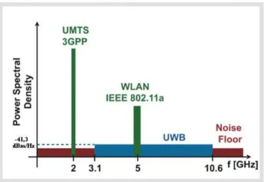
Ultra-wideband is a radio technology. It can be used at very low energy levels for short-range high-bandwidth communications by using a larger portion of the radio spectrum. This method is using pulse coded information with sharp carrier pulses at a bunch of center frequencies in logical connex. UWB has traditional applica-tions in non cooperative radar imaging. Most recent applicaapplica-tions target sensor data collection, precision locating and tracking applications. Ultra Wideband was tra-ditionally accepted as pulse radio, but the FCC and ITU-R now define UWB in terms of a transmission from an antenna for which the emitted signal bandwidth exceeds the lesser of 500 MHz or 20% of the center frequency. Thus, pulse-based systems (wherein each transmitted pulse instantaneously occupies the UWB band-width, or an aggregation of at least 500 MHz worth of narrow band carriers, for example in orthogonal frequency division multiplexing (OFDM) fashion) can gain access to the UWB spectrum under the rules [1] [2]. Pulse repetition rates may be either low or very high. Pulse-based radars and imaging systems tend to use low repetition rates, typically in the range of 1 to 100 megapulses per second. On the other hand, communications systems favor high repetition rates, typically in the range of 1 to 2 giga-pulses per second, thus enabling short range gigabit-per-second communications systems. Each pulse in a pulse-based UWB system occupies the entire UWB bandwidth, thus reaping the benefits of relative immunity to multipath fading (but not to intersymbol interference), unlike carrier-based systems that are subject to both deep fades and intersymbol interference. A February 14, 2002 Re-port and Order by the FCC authorizes the unlicensed use of UWB in 3.1÷10.6 GHz.
The FCC power spectral density emission limit for UWB emitters operating in the UWB band is -41.3 dBm/MHz. This is the same limit that applies to unintentional emitters in the UWB band, the so called Part 15 limit (figure 1). However, the
emis-Figure 1.1: Electromagnetical spectrum occupied by UWB signals
sion limit for UWB emitters can be significantly lower (as low as -75 dBm/MHz) in other segments of the spectrum. Due to the extremely low emission levels currently allowed by regulatory agencies, UWB systems tend to be short-range and indoors applications. However, due to the short duration of the UWB pulses, it is easier to engineer extremely high data rates, and data rate can be readily traded for range by simply aggregating pulse energy per data bit using either simple integration or by coding techniques. Conventional OFDM technology can also be used subject to the minimum bandwidth requirement of the regulations. High data rate UWB can enable wireless monitors, the efficient transfer of data from digital camcorders, wire-less printing of digital pictures from a camera without the need for an intervening personal computer, and the transfer of files among cell phone handsets and other handheld devices like personal digital audio and video players.
1.2
Synchronization in UWB
In any communication system, the receiver needs to know the timing information of the received signal to accomplish demodulation. The subsystem of the receiver which performs the task of estimating this timing information is known as the syn-chronization stage. Synsyn-chronization is an especially difficult task in spread spectrum systems which employ spreading codes to distribute the transmitted signal energy
over a wide bandwidth. The receiver needs to be precisely synchronized to the spreading code to be able to despread the received signal and proceed with demod-ulation. Timing acquisition is a particularly acute problem faced by UWB systems [3], as explained in the following. Short pulses and low duty cycle signaling employed in UWB systems place stringent timing requirements at the receiver for demodu-lation. The wide bandwidth results in a fine resolution of the timing uncertainty region, thereby imposing a large search space for the acquisition system. More-over, the transmitted pulse can be distorted through the antennas and the channel, and hence the receiver may not have exact knowledge of the received pulse signal waveform. Typical UWB channels can be as long as 200 ns [4] [5], and can be characterized by dense multipath with thousands of components for some NLOS scenarios. The transmit-reference (TR) scheme first proposed for UWB in [6] [7] emerges as a realistic candidate that can effectively deal with these challenges. By transmitting pulses in pairs (or doublets) in which both pulses are distorted by the same channel, and using an autocorrelation receiver, the total energy of the chan-nel is gathered to detect the signal without having to estimate individual chanchan-nel multipath components. The simple delay (at the transmitter), correlation and in-tegration operations (at the receiver) ease the timing synchronization requirements and reduce the transceiver’s complexity.
In this thesis a TR-UWB Communication System is considered. Transmitted Ref-erence UWB uses ultra-short information bearing pulses and thus promises high speed, high precision, resolved multipath and simpler receiver structures.
The same system was considered by Andreas Schranzhofer in his Master’s Thesis [8] at TU Delft. He proposed to make synchronization by correlating the received samples with the code sequence known at the receiver. It’s the traditional ”matched filter”. The limitation in [8] is that it assumes there is no Inter Symbol Interference (ISI) or Inter Frame Interference (IFI).
In [9] another acquisition scheme is proposed, in which, two sets of direct sequence code sequence are used to facilitate coarse timing and fine aligning. In this case, no IFI is assumed. A very complex algorithm is proposed in [10]. It proposes a blind synchronization method for TR-UWB systems. The matrix decomposition brings to a very high complexity. In the CAS group, a new algorithm is proposed, claimed able to solve the presence of IFI, with a very low complexity. The thesis focuses on the new proposed algorithm.
Mathematical notation
v boldface uncapitalized characters denote vectors
M boldface capitalized characters denote matrices ˜
v, ˜M the operator˜means the FFT of the vector/matrix
x, A italic characters denote scalars or complex numbers
bxc denotes the first integer smaller than x
⊗ denotes the Kronecker product of two matrices
¯ denotes the Schur-Hadamard product of two matrices
Chapter 2
Data Model
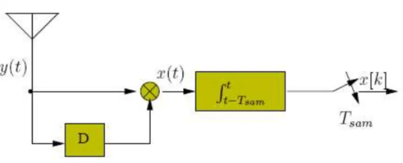
Figure 2.1: Autocorrelation receiver
This chapter presents the data model as described in [11]. Let’s start introducing the model of a single frame, of duration Tf. Then we’ll extend the model to multiple
frames and multiple symbols.
2.1
Single frame
When a UWB pulse g(t) is transmitted, it usually undergoes a distortion due to the UWB physical channel hp(t), supposed to be of finite length Th. The signal is
picked up by the antenna receiver, whose impulse response is a(t). Consequently the expression of the received signal is:
h(t) comprises the communication channel, the transmitted pulse and the antenna
response. Actually, it hasn’t been considered the bandpass filter present after the antenna receiver, but a(t) could be seen also as the convolution between the antenna response and the bandpass filter response. Anyway, from now on, we’ll consider h(t) as the ”composite” channel response. In TR-UWB systems, the signal is transmitted sending a pair of pulses per frame, called doublet. The first pulse of each doublet is fixed, called reference pulse, whereas the second pulse, sent after D seconds from the first, is the data pulse and its polarity s0 contains the information: s0 ∈ {−1, +1}.
The expression of the signal due to one transmitted frame, after the antenna receiver and the bandpass filter is therefore:
y0(t) = h(t) + s0· h(t − D)
In figure 2.1 the receiver structure (leaving out the bandpass filter) is shown. As we can se, y0(t) undergoes a multiplication by a delayed version (by D seconds) of
itself. After that, the result is integrated and dumped. The sampling period is Tsam
and it usually is an oversampling, since P samples per frame are taken. P is called ”oversampling factor”: Tsam = TPf.
The expression of the signal at the multiplier’s output is
x0(t) = y0(t)y0(t − D)
= [h(t) + s0h(t − D)][h(t − D) + s0h(t − 2D)]
= [h(t)h(t − D) + h(t − D)h(t − 2D)] + s0[h2(t − D) + h(t)h(t − 2D)]
Let’s define the channel autocorrelation function as
R(τ, n) =
Z nTsam
(n−1)Tsam
h(t)h(t − τ )dt.
x0[n] = [R(0, n − D Tsam ) + R(2D, n)]s + [R(D, n) + R(D, n − D Tsam )] (2.2) In equation (2.2) R(0, n − D
Tsam) contains the energy of the channel, in the time
in-terval [(n − 1)Tsam, nTsam]. Let’s consider a certain correlation length τ0: as shown
in [11], when τ0 < D we can neglect the other terms of equation (2.2). Usually τ0
is very small, often smaller than the delay D. Therefore we can ignore the terms
R(τ, . . .) with τ ²{D, 2D}. For the sample x0[n + 1] the time interval involved is
[nTsam, (n + 1)Tsam]: we can look at the oversampling process as a segmentation of
the channel in ”sub-channels”, because Tsam < Tf < Th. For each segment we have
a channel autocorrelation function and a dominant term R(0, . . .) that contains the energy of the sub-channel. Since Th is the length of the physical channel, we’ll have
Ph segments, where Ph = bTT hsamc. From now on, Ph samples will describe the original
composite channel response:
h[n] =
Z nTsam
(n−1)Tsam
h2(t)dt n = 1, . . . , Ph (2.3)
So, we can Define a TR-UWB ”channel” vector:
h = [h[1], . . . , h[Ph]]T (2.4)
We can stack the discrete samples in a vector x0, obtaining:
x0 = h · s0+ noise (2.5)
This model is a simple approximation for single frame. It reduces the complexity, even for the receiver algorithms and was shown that the approximation doesn’t produce any considerable loss in the BER performance. It is due to the statistical properties of the UWB channels and to the nature of the UWB signal.
2.2
Multiple frames
Let’s consider now the transmission of Nf consecutive frames, each one with
dura-tion Tf and for each one the preceding data model is valid. Now, the data pulse
of each doublet carries the information of a symbol: a data bit sj modulates the
polarity of the second pulse of the frame number j. We can now also introduce the presence of inter-frame interference (IFI), since the duration of each frame Tf is
shorter than the channel length Th.
We use a single delay for all the frames, that is D seconds, so that the receiver structure is the same as in figure 2.2. We have now new cross terms in the result of the integration and dumping, because there are more than one frame. They still are terms of the autocorrelation functions of the channel segments and they also can be ignored since the correlation length in these cross-terms are much longer than Tf.
What we cannot ignore is the new matched terms that spread over some next frames, due to the fact that Th > Tf. These other matched terms produce IFI. Let’s define
a channel matrix H to model the multiple frames case:
x = Hs + noise (2.6)
where x contains all the received samples, s is the unknown data vector
s = [s1, . . . , sNf]
T
The channel matrix H has the structure shown in figure 2.2. The first thing to notice is the presence of shifted version of h defined in (2.4). Then, let’s notice also the effect of IFI, looking at how many rows in H have more than one entry different by zero.
2.3
Effect of timing synchronization
In UWB communication systems, as already said, the pulses have very short du-ration. It makes the synchronization have stringent requirements. To solve the problem we work in the digital domain, elaborating the samples received. So, the analog part of the receiver can be kept data-independent.
Let’s suppose to receive the data packet (consisting of multiple frames) with an off-set G at the beginning, which means, in other words, that we are not synchronized.
Figure 2.2: Data model for multiple frames
The expression of the offset is:
G = G0T
sam+ g
where G0 is an integer and g respects the condition: 0 < g < T
sam. We can
incor-porate the integer G0 in the data model putting G0 rows at the top of the channel
matrix H with all elements equal to zero. However we still have to include the offset fraction g and we can do it redefining the channel vector h as follows:
h[n] =
Z nTsam
(n−1)Tsam
h2(t − g)dt, n = 1, . . . , P
h
Actually, we didn’t any assumptions on the unknown channel vector h, so, the model (2.6) is still valid. In the chapter 3, we’ll explain the algorithm to estimate the delay
2.4
Multiple frames, Multiple symbols - Single
User case
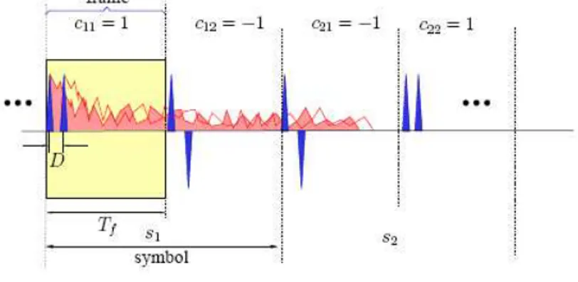
Let’s go now to extend the preceding models to the multiple frames and multi-ple symbols case. Let’s suppose to transmit a packet of Ns data symbols s =
[s1, . . . , sNs]
T, where each symbol s
i²{−1, +1} is composed of Nf frames, whose
du-ration is still Tf. In each frame, the pulses are separated by D seconds. Let’s suppose
then cij²{−1, +1}, j = 1, . . . , Nf to be the known user code of the frame number
j in the symbol number i. It means that the code can varie from frame to frame
and from symbol to symbol. The structure of the receiver is still shown in figure 2.1 and the structure of the transmitted pulse sequence is shown in figure 2.3.
Figure 2.3: Pulse sequence structure
The expression of the signal after the antenna receiver and the pass-band filter, without noise, is:
y(t) = Ns X i=1 Nf X j=1 [h(t−((i−1)Nf+j −1)Tf)+sicijh(t−((i−1)Nf+j −1)Tf−D)] (2.7) where ci = [ci1, . . . , ciNf]
T is the code vector for the i−th symbol s
i. Then we have
the multiplication x(t) = y(t)y(t − D), the integration and dumping with oversam-pling factor P = Tf/Tsam. As said in the section 2.1, The unmatched terms and
the cross-terms can be neglected. The data model in (2.6) can be easily extended to include the code cij.
We still stack the samples x[n] = RnTsam
(n−1)Tsamx(t)dt, n = 1, . . . , (NsNf − 1)P +
x = Hdiag{c1, . . . , cNs}s + noise (2.8)
where, H still have the same structure shown in fig. 2.2, and the ’diag’ operator puts the vectors c1, . . . , cNs into a block diagonal matrix. We can also rewrite the
Figure 2.4: The data model for the single user case with no offset
data model in (3.1) as,
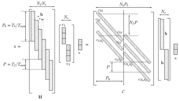
x = C(INs⊗ h)s + noise (2.9)
where ⊗ denotes the Kronecker product and C is the code matrix of size
((NfNs− 1)Tf + Th)/Tsam× (ThNs)/Tsam
The structure of x is shown in figure 2.4, where we can see also the structure of the matrix C.
As we said at the end of section 2.3, in the following chapter, the data model will be modified to introduce the the offset and illustrate the algorithm to solve the synchronization.
Chapter 3
The synchronization algorithm
A synchronization algorithm is proposed in this chapter. It was developed by Yiyin Wang, PhD student in the group of Circuits and Systems at TU-Delft. The main ad-vantage of this algorithm is to solve the IFI problem in the synchronization through the code sequence deconvolution done in frequency domain. The traditional code match filter can’t handle IFI. It requires the frame length to be long enough to let the channel die out before the next frame is transmitted. The proposed algorithm has lower complexity than the code match filter. The novel algorithm facilitates higher data rate communication and reduces the acquisition time. Yiyin Wang is now improving the algorithm as we can see in [12].
3.1
Data model
The scenario here is to solve the synchronization problem for single user with single delay. The received Ns symbols at the antenna output without noise can be
mod-eled as in equation (2.7). The proposed training sequence has the following property:
sk= sk+1 = sk+2 = . . . = sk+Ns
As already said, the duration of the channel Th is much longer than the frame time
Tf. This assumption introduces Inter Frame Interference. To avoid Inter Symbol
Interference we insert a guard interval between two following symbols. The guard interval is equal to Th− Tf. The integration and the oversampling (remember figure
x[n] =
Z nTsam
(n−1)Tsam
y(t)y(t − D), n = 1, . . . , NsLs (3.1)
where Ls= NfP + Ph− P is the symbol length in terms of number of samples (see
figure 3.1).
Figure 3.1: Samples per symbol period
x[n] is stacked into a column vector as described in the chapter 2:
x = C(I ⊗ h)s = Hdiag{c1, . . . , cNs}s (3.2)
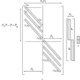
Here C is slightly different from C in chapter 2, there is no overlap between symbols in C, due to the guard interval inserted. See figure 3.2:
Figure 3.2: The data model
H in the equation (3.2) is a NsLs× NsNf matrix composed by the h vector. c1,
c2, . . ., cNs are the code vectors of each symbol. Nevertheless, as we said, we have
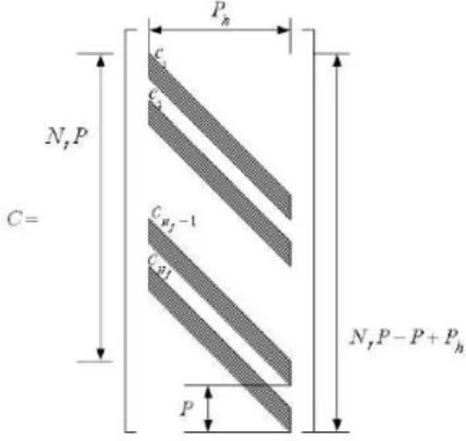
the same code vector for each symbol, so we can call every code vector as c, whose entries are c1, c2, . . . , cNf. In this case the matrix C in figure 3.2 contains replicas of
the code matrix C, whose structure is shown in figure 3.3
Figure 3.3: Code matrix C
3.1.1
Asynchronous single user model
Without loss of generality, the unknown timing offset τa is in one symbol range,
τa ∈ [0, Nf ∗ Tf + Th− Tf) (3.3)
We can also write τa= naTsam+Tr, where na ∈ {0, 1, . . . , Nf∗P +(Th−Tf)/T f ∗P }
and 0 ≤ Tr < Tsam is the tracking error. As said in section 2.3, the tracking error Tr
can be absorbed in the unknown channel vector. So, in terms of samples, equation (3.3) becomes:
τ ∈ {0, 1, . . . , Ls− 1} (3.4)
Let’s notice that this assumption means that, stacking the first Ls received samples
into a column vector, at least one of them belongs to the transmitted symbol: if
τ = 0 , all the Ls samples are related to one symbol. If τ = Ls− 1 , only the last
adjacent symbol periods. Stacking 2Ls data samples into a column vector to model
a single symbol, we would obtain: x[k] ... x[k + 2Ls− 1] = Cτhsk = 0τ C 0r 2Ls×Ph hsk (3.5)
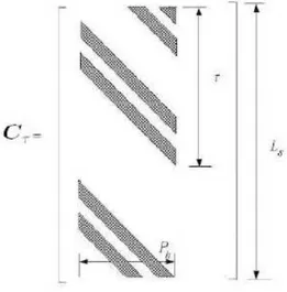
Cτ is made up of three blocks. C is the known user code matrix, already shown
in figure 3.3. 0τ is τ rows of 0. 0r is Ls− τ rows of 0. sk is the kth symbol. But
if we stack the samples into column vectors of Ls elements each one, we need two
columns to describe one symbol:
x[k] x[k + Ls] ... ... x[k + Ls − 1] x[k + 2Ls− 1] = CsτHS = = [C00τ C0τ] " h 0 0 h # " 0 sk sk 0 # (3.6)
where Csτ is a Ls× 2Ph matrix. It’s made up of two blocks. The first Ph columns
constitute the matrix C00τ and the last Phcolumns form the matrix C
0
τ. In the matrix
C00τ the first τ rows are the last τ rows of the matrix C. The other elements are all 0’s. In the matrix C0τ the last Ls− τ rows are the first Ls− τ rows of the matrix C
and the other elements are 0’s. See figure 3.4.
Now, remembering that the training sequence is composed of symbols all equal, we stack the received samples in a Ls× Ns matrix X, extending the model in the
Figure 3.4: Code matrix Csτ X = x[k] x[k + Ls] . . . x[k + (Ns− 1)Ls] ... ... ... ... x[k + Ls− 1] x[k + 2Ls− 1] . . . x[k + NsLs− 1] = CsτHS = h C00τ C0τ i" h 0 0 h # " sk sk+1 sk+2 . . . sk+Ns−1 sk+1 sk+2 sk+3 . . . sk+Ns #
Let’s remember that the symbols in the training sequence are equal to 1 (and notice that the training sequence is composed by Ns+ 1 symbols, but the synchronization
algorithm is applied on Ns symbol periods). In this case:
X = h C00τ C0τ i" h 0 0 h # " 1 1 1 . . . 1 1 1 1 . . . 1 # 2×Ns = h C00τ C0τ i" h 0 0 h # " 1 1 # 1T
Where 1T is a row vector composed by N s 1’s X = h C00τh C0τh i" 1 1 # 1T = [Cτ] h1T (3.7)
Cτ is a circular shift of τ rows of the matrix C0: figure 3.5
Figure 3.5: Code matrix Cτ
3.2
Synchronization algorithm
We can utilize the shift invariance property that a delay in time domain corresponds to a phase shift in frequency domain for the cyclic block Cτ: Let’s define ˜Cτ = FCτ
and ˜C0 = FC0, where the operator F is the FFT operation (it’s a Ls× Ls FFT
matrix). So, ˜Cτ is the DFT of Cτ whereas ˜C0 is the DFT of C0. Let’s notice that
the matrix C0 is the matrix C
˜ Cτ = ˜C0¯ [φτ, . . . , φτ] (3.8) where φτ = [1, e− j2πτ Ls , . . . , (e− j2πτ Ls )Ls−1]T.
Since each column Cτ is just one sample shift of the previous column, we can rewrite
the formulation (3.8) as
˜
Cτ = ˜c011
T ¯ [φ
τ φτ +1 . . . φτ +Ph−1] (3.9)
where 1 is a Ph length vector with all entries equal to 1 and c01 is the first
col-umn of the code matrix C0, so that ˜c01 is the first column of ˜C0. Let’s define
˜
Xi, i = 0, . . . , Ls− 1 the elements of ˜c01. They are the components of the FFT of
c01: ˜ Xi = NXf−1 m=0 cme−j2π mP i Ls (3.10)
because, the column c01 is:
c01 =
£
c0 0 0 c1 0 0 c2 0 . . . cNf−1 0 . . . 0 0
¤T
Ls
where, between two adjacent chips there are (P − 1) 0’s. Let ˜Cinv = [diag(˜c01)]−1:
˜ Cinv = 1 ˜ X0 0 0 . . . 0 0 1 ˜ X1 0 0 ... 0 0 1 ˜ X2 0 ... ... ... ... ... ... 0 0 0 0 1 ˜ XLs−1 Ls×Ls
We can estimate the offset τ by the following way:
˜
CinvC˜τ = [φτ φτ +1 . . . φτ +Ph−1] (3.11)
F−1C˜ invC˜τ = F−1[φτ φτ +1 . . . φτ +Ph−1] = 0τ IPh 0r Ls×Ph (3.12)
0τ is a τ × Ph matrix, with null elements. IPh is a Ph× Ph identity matrix. 0r is a
r × Ph matrix with null elements. This means that τ is equal to the number of rows
of the matrix 0τ. (If τ + Ph is bigger than Ls then the structure is a bit different: in
the matrix resulting by the equation (3.12), the first τ + Ph− Ls rows are the last
τ + Ph− Ls rows of IPh and the last Ls− τ rows are the first Ls− τ rows of IPh. In
the middle there is the matrix 0τ). We can understand the result of equation (3.12)
rewriting it as: F−1C˜ invC˜τ = = F−1 1 ˜ X0 0 0 . . . 0 0 1 ˜ X1 0 0 ... 0 0 1 ˜ X2 0 ... ... ... ... ... ... 0 0 0 0 1 ˜ XLs−1 ˜ X0 ˜ X1 ˜ X2 ... ˜ XLs−1 ¯ [φτ φτ +1 . . . φτ +Ph−1] = = F−1 1 1 1 ... 1 ¯ [φτ φτ +1 . . . φτ +Ph−1] = = F−1[φτ φτ +1 . . . φτ +Ph−1] = = 0τ IPh 0r Ls×Ph
Let’s now apply the operation described till now to the data matrix, built with the collected samples, as in the equation (3.7):
F−1C˜ invFX = F−1C˜invFCτh1T (3.13) = F−1C˜ invC˜τh1T = 0τ IPh 0r h1T = 0τ h 0r 1T (3.14)
(Again, if τ + Ph > Ls the matrix in equation (3.14) is a bit different:
h00 0τ h0 1T
where h00 is the last Ph − (Ls− τ ) elements of vector h and h
0
is the first Ls− τ
elements of h).
Define the vector y = F−1C˜
invFX1: y = 0τ Nsh 0r (3.15)
we get the estimation of the offset:
ˆ τ = argmaxτ( 1 Ns Lw X n=1 y[τ + n]) , τ = 0, 1, . . . , Ls− 1 (3.16)
we sum all the elements in that window.The selection of Lw depends on the channel
energy profile and the SNR: it should be a length which can include the part with the highest channel energy to noise ratio.
Chapter 4
The modified algorithm
The algorithm described in the chapter 3 was developed by Yiyin Wang, Geert Leus and Alle-Jan van der Veen. Some aspects are being improved. In this chapter we describe one problem in the algorithm and a simple practical way to solve it, modifying slightly the matrix ˜Cinv.
4.1
Noise analysis
Let’s start analyzing the noise. In the equation (3.13) we didn’t consider the noise. Now, let’s suppose that at the antenna RX we receive the signal convolved with the channel plus White Gaussian Noise. After the first part of the receiver, the analog part, we go to integrate and dump obtaining signal plus noise samples. As we have already said, we stack the received data in the matrix X, but now we define also the noise samples matrix N :
n[k] n[k + Ls] . . . n[k + (Ns− 1)Ls] ... ... ... ... n[k + Ls− 1] n[k + 2Ls− 1] . . . n[k + NsLs− 1] Ls×Ns
These samples are Independent Gaussian Variables, with the same mean value 0 and the same variance σ2. This assumption has been demonstrated in [13] by Hoctor
and Tomlinson. The noise matrix will undergo the same operations undergone by the matrix X. First of all the FFT operation, obtaining the matrix ˜N :
˜ N = ˜ nk[0] ˜nk+Ls[0] . . . n˜k+(Ns−1)Ls[0] ... ... ... ... ˜ nk[Ls− 1] ˜nk+Ls[Ls− 1] . . . ˜nk+(Ns−1)Ls[Ls− 1] Ls×Ns where ˜ nk[i] = LXs−1 n=0 nk+ne−j2π ni Ls , i = 0, 1, . . . , 2Ls− 1 (4.1)
The sum of indipendent Gaussian Variables is still a Gaussian Variable. Its mean value is the sum of all mean values, so it’s 0. Let’s calculate the variance:
σn2˜k[i] = E{(˜nk[i]) · (˜nk[i])∗}
= E{( LXs−1 n=0 nk+ne−j2π ni Ls) · ( LXs−1 l=0 nk+le−j2π li Ls)∗} = E{ LXs−1 n=0 LXs−1 l=0 nk+nn∗k+le−j2π ni Lsej2πLsli} = LXs−1 n=0 LXs−1 l=0 E{nk+nn∗k+l}e−j2π ni Lsej2πLsli
We know that the variables are independent, so E{nk+nn∗k+l} 6= 0 only for l = n:
σ2 ˜ nk[i] = LXs−1 n=0 E{|nk+n|2} = LXs−1 n=0 σ2 = L sσ2 (4.2)
So, each element of ˜N is a Gaussian variable with mean value 0 and variance Lsσ2.
˜ N0 = ˜CinvN =˜ (4.3) = 1 ˜ X0 0 0 . . . 0 0 1 ˜ X1 0 0 ... 0 0 1 ˜ X2 0 ... ... ... ... ... ... 0 0 0 0 1 ˜ XLs−1 ˜ nk[0] ˜nk+Ls[0] . . . n˜k+(Ns−1)Ls[0] ... ... ... ... ˜ nk[Ls− 1] ˜nk+Ls[Ls− 1] . . . ˜nk+(Ns−1)Ls[Ls− 1] = ˜ nk[0] ˜ X0 ˜ nk+Ls[0] ˜ X0 . . . ˜ nk+(Ns−1)Ls[0] ˜ X0 ... ... ... ... ˜ nk[Ls−1] ˜ XLs−1 ˜ nk+Ls[Ls−1] ˜ XLs−1 . . . ˜ nk+(Ns−1)Ls[Ls−1] ˜ XLs−1 Ls×Ns
And finally we apply the IFFT to this matrix, obtaining the matrix that we call N0:
N0 = F−1N˜0 = F−1C˜ invN˜ = n0 k n0k+Ls . . . n 0 k+(Ns−1)Ls n0 k+1 n0k+Ls+1 . . . ... ... ... ... ... n0 k+Ls−1 n 0 k+2Ls−1 . . . n 0 k+NsLs−1 Ls×Ns
where, for the first column entries we have:
n0 k+m= 1 Ls LXs−1 i=0 ˜ nk[i]ej2π mi Ls , m = 0, 1, . . . , Ls− 1
It’s the same for the other columns: for example for the second column we have to write: n0 k+Ls+m= 1 Ls LXs−1 i=0 ˜ nk+Ls[i]e j2πmi Ls , m = 0, 1, . . . , Ls− 1
matrix N , which has independent Gaussian variables as elements. In fact, we apply the IFFT to the matrix ˜N0 = ˜CinvN , but the matrix ˜˜ Cinv is a deterministic
quan-tity: it means that the elements in the matrix N0 are still independent Gaussian variables. They still have the same mean value equal to 0. But now the variance of each element is different from the others. So, let’s calculate the variance of each element of the matrix N0:
σ2 n0 k+m = E[(n 0 k+m) · (n0k+m)∗] (4.4) = E[ 1 (Ls)2 ( LXs−1 i=0 ˜ nk[i] ˜ Xi ej2πimLs)( LXs−1 t=0 ˜ n∗ k[t] ˜ X∗ t e−j2πtmLs)] = E[ 1 (Ls)2 ( LXs−1 i=0 PLs−1 n=0 nk+ne−j2π ni Ls ˜ Xi ej2πimLs) · ·( LXs−1 t=0 PLs−1 l=0 n∗k+le+j2π lt Ls ˜ X∗ t e−j2πtmLs)] = 1 (Ls)2 LXs−1 i=0 LXs−1 t=0 PLs−1 n=0 PLs−1 l=0 E[nk+nn∗k+l]e−j2π ni−lt Ls ˜ XiX˜t∗ ej2πm(i−t)Ls = 1 (Ls)2 LXs−1 i=0 LXs−1 t=0 PLs−1 n=0 E[|nk+n|2]e−j2π n(i−t) Ls ˜ XiX˜t∗ ej2πm(i−t)Ls = 1 (Ls)2 LXs−1 i=0 LXs−1 t=0 PLs−1 n=0 σ2e−j2π n(i−t) Ls ˜ XiX˜t∗ ej2πm(i−t)Ls = σ 2 (Ls)2 LXs−1 n=0 ( LXs−1 i=0 1 ˜ Xi e+j2π(m−n)iLs LXs−1 t=0 1 ˜ X∗ t e−j2π(m−n)tLs ) = σ 2 (Ls)2 LXs−1 n=0 [( LXs−1 i=0 1 ˜ Xi e+j2π(m−n)iLs )( LXs−1 t=0 1 ˜ Xt e+j2π(m−n)tLs )∗] = σ2 (Ls)2 LXs−1 n=0 | LXs−1 i=0 1 ˜ Xi e+j2π(m−n)iLs |2 ≤ σ 2 Ls LXs−1 i=0 1 | ˜Xi|2 (4.5)
As we can see, the variance changes elements by elements and also the value is different for different code sequences. We can only say that in the matrix N0 the
mth element of each column has the same variance as the mth element of each other
column. Looking at equation (4.5), we realize that the most important result is that now we know that the variance could increase as the inverse of the norm of the components ˜Xi becomes larger. We would like to have components ˜Xi with norm
high enough to avoid that the variance of the noise becomes too high.
4.2
Error probability and MSE
In order to understand the advantage to have components ˜Xi with high norm, we
must analyze how the variance of the noise influences the estimation of the offset τ . Remembering the formula (2.16), now we introduce also the noise. So, the vector y now contains also noise. In fact, define:
Z = X + N
we apply all the operations described before to the matrix Z:
F−1C˜ invFZ = F−1C˜invF(X + N ) = F−1C˜invFX + F−1C˜invFN = 0τ IPh 0r h1T + N0 Let’s define v(τ ) = 1 Ns Tw X n=1 y[τ + n] , τ = 0, . . . , Ls− 1 and
v = [v(0) v(1) . . . v(Ls− 1)]
remembering the formula (3.16) and supposing that the offset is equal to τ0, we have
the correct estimation when v(τ0) is the maximum element of the vector v. We must
calculate the statistics of v(τ0).
v(τ0) = Lw X n=1 Ã h[n − 1] + 1 Ns NXs−1 i=0 n0 k+τ0+(n−1)+iLs ! (4.6)
v(τ0) is the sum of a deterministic variable
PLw
n=1h[n − 1] plus the sum of LsNs
independent gaussian variables with zero mean value and different variances. So,
v(τ0) is still a gaussian variable with mean value equal to
PLw
n=1h[n−1] and variance
equal to the sum of the variances of the LsNs noise elements, divided by Ns2. When
τ differs from τ0, the reasoning is exactly the same, but the mean value is smaller
and the variance is different, because, as shown in section 2.1, the elements of matrix
N0 have in general different variances. We can write:
v(τ0) ∈ N (µτ0, σ 2
τ0)
v(τ ) ∈ N (µτ, σ2τ) , τ = 0, 1, . . . , Ls− 1 τ 6= τ0
where we know only that µτ0 is bigger than µτ, for τ 6= τ0. The estimation of the
offset is correct when
v(τ0) > v(τ ), τ = 0, 1, . . . , Ls− 1 τ 6= τ0 (4.7)
1 − P r{error} = 1 − (P r{v(0) > v(τ0)} + . . . + P r{v(Ls− 1) > v(τ0)}) = 1 − (P r{v(0) − v(τ0) > 0} + . . . + P r{v(Ls− 1) − v(τ0) > 0}) = 1 − (Q µτ0 − µ0 1 Ns q σ2 τ0+ σ 2 0 + . . . + Q µτ0 − µLs−1 1 Ns q σ2 τ0 + σ 2 Ls−1 ) = 1 − LXs−1 τ =0 τ 6=τ0 Q Ã µτ0 − µτ 1 Ns p σ2 τ0 + σ 2 τ ! (4.8)
The result of equation (4.8) makes us understand the importance to have small vari-ances. We can also calculate the normalized Mean Squared Error of the estimation of the offset as:
MSE = E "µ ˜ τ − τ0 Ls ¶2# = LXs−1 τ =0 P r(˜τ = τ ) µ τ − τ0 Ls ¶2 (4.9)
To calculate the probabilities P r(˜τ = τ ) of each term in the summation in equation
(4.9) we have just to notice that they have similar expressions as the probability of correct estimation (4.8). We arrive to the same conclusion: we want to have small variances of the noise elements in the matrix N0. If we generate the code sequence
randomly, as a random sequence of +1 and -1, we don’t have any control on the consequences. This means that we could have also components ˜Xi with very small
norm, also equal to 0 in some cases. In the next section we’ll describe a practical method to avoid this problem, also keeping the code sequences randomly generated.
4.3
The solution: replacement of components
The first approach to solve the problem described in the preceding section was to work on the design of the code sequences. The idea was to propose a particular con-figuration for the code sequences, maybe also redefining the set of values to which the chips belong, for example, a particular set of complex numbers with certain phases and certain norms. The goal of the new design was to avoid to produce DFT vectors with components with too small norms. The problem met during this approach
is the following: the FFT depends on many parameters and even if we find a se-quence that produces a DFT with components characterized by norms high enough, the same sequence could produce a completely different result when the parameters change. In fact, remembering the equation (3.10), we notice that ˜Xi depends on the
parameters P, Ph, Nf (Ls = (Nf − 1)P + Ph). Changing one of them, we change the
result of the FFT. Actually there exist some code sequence that produce DFT with constant norms. But in our algorithm we apply the FFT operation to a vector that is a bit different by the transmitted code sequence. In fact, let’s suppose that the vector
c = [c0 c1 c2 . . . cNf−1]
is a sequence that has a DFT with constant norms. In our algorithm the FFT oper-ation is applied to the first column of the matrix C0. This column has the following
structure: c01 = £ c0 0 0 c1 0 0 c2 0 . . . cNf−1 0 . . . 0 0 ¤T Ls
It’s not just an oversampling of the vector c, because between two chips there are (P − 1) 0’s, but after the last chip cNf−1 there are Ph− 1 0’s. It would be an
over-sampling if Ph = P . But this means that we wouldn’t have Inter Frame Interference,
because Ph = P means Th = Tf whereas we made the assumptions that we have
IFI and Th could be also À Tf. If c01 was just an oversampling of c we would
have a DFT with still with constant norms. But in reality, we don’t have just an oversampling and in fact the DFT changes completely.
The solution was found following another approach. The idea was simply to replace those components ˜Xi that are too small, compared with the other components. In
fact, the ideal situation is when all the frequency components have more or less the same energy, around a certain mean value. But there are situations in which some components have too small energy and this means that the variance could become too high, as we can understand looking at (4.5). So, the idea is to calculate the FFT of the column vector c01. Then calculate the inverse of each components ˜Xi.
After that, set a threshold under a certain criteria and finally replace the elements
1 ˜
Xi, that are over the threshold, with another element (for example 0). In this way
we’ll reduce the value of the variances of the elements in N0, but we’ll generate also
as described: instead of the matrix ˜Cinv of equation (3.12), now we have the matrix ˜ Cinv new ˜ Cinv new = 1 ˜ X0 0 0 0 . . . 0 0 0 0 0 . . . ... 0 0 1 ˜ X2 0 . . . ... ... ... ... ... ... ... 0 0 0 . . . 1 ˜ XLs−2 0 0 0 0 . . . 0 0
In this example we replaced the elements 1 ˜
X1 and 1 ˜
XLs−2 with 0’s. Let’s substitute in
equation (3.12) the matrix ˜Cinv with ˜Cinv new:
˜ Cinv newC˜τ = (4.10) = 1 ˜ X0 0 0 . . . 0 0 0 0 . . . ... 0 0 1 ˜ X2 . . . ... ... ... ... ... ... 0 0 0 . . . 0 ˜ X0 ˜ X1 ˜ X2 ... ˜ XLs−1 1T ¯ [φτ φτ +1 . . . φτ +Ph−1] = 1 0 1 ... 1 0 1T ¯ [φ τ φτ +1 . . . φτ +Ph−1] = 1 1 1 ... 1 1 − 0 1 0 ... 0 1 1T ¯ [φ τ φτ +1 . . . φτ +Ph−1]
= 1 1 1 ... 1 1 1T ¯ [φ τ φτ +1 . . . φτ +Ph−1] − 0 1 0 ... 0 1 1T ¯ [φ τ φτ +1 . . . φτ +Ph−1]
Then, applying the IFFT, we obtain the same result as before, plus a new matrix that we call M : ˜ Cinv newC˜τ = 0τ IPh 0r + M (4.11) where: M = F−1 − 0 1 0 ... 0 1 1T ¯ [φ τ φτ +1 . . . φτ +Ph−1] (4.12) = F−1©−ε · 1T ¯ [φ τ φτ +1 . . . φτ +Ph−1] ª
F−1{ ˜C inv newFX} = = 0τ IPh 0r + M h1T = 0τ h 0r 1T + ∆ (4.13) where ∆ = M h1T (4.14)
The matrix ∆ depends on the number of components that we replace and also the way to replace these components. In fact replacing the component 1
˜
Xi with 0 is not
the best choice. To set the threshold and also to define the new elements to put in the matrix ˜Cinv new, we should follow some criteria, as zero forcing or a criteria to
minimize the MSE, or something else. In this thesis a practical method to generate the matrix ˜Cinv new is proposed, looking at values that we obtain by simulations.
Observing the norms of the components 1 ˜
Xi we have noted that in every case,
chang-ing sequences and parameters, we don’t have many components that become too high, compared to the total number of components. It means that the vector ε in (4.12) will have few elements different than 0, compared to the total number of ele-ments. But now we should understand what does high components mean. We need a threshold and then define too high the components 1
˜
Xi that have a norm bigger
than the threshold. The proposed method is to treat the norms of the components
1 ˜
Xi as random variables with a certain average and a certain standard deviation. We
have good sequences when the energy of the frequency components of c01 is more
or less the same, around a certain mean value. Otherwise, a bad sequence produces a vector c01 that has some frequency components too small and this means to have
u = ½ 1 | ˜Xi| ¾Ls−1 i=0
We have also to remember that the same sequence could be bad or good, changing some parameters P, Ph, Nf.
So, for each sequence u, we calculate the average and the standard deviation of the elements. Then we set the threshold: looking at the results of the simulations, we found the best threshold was equal to the average plus standard deviation. Finally we replace those components having norm bigger than the threshold with new com-ponents that have the same phases but norms equal to the average. This choice is due to the fact that we want to have a matrix ∆ with negligible values and replacing the components with zero is a poor choice, besides besides that it is not necessary. The last thing that we have to understand is that the peaks that really can increase the variance of the noise samples are present in those vectors u in which more or less the values are all around the mean value, except on these few peaks. Otherwise, we can also have many peaks but not so high to worsen the performance really. The following figure helps to understand:
0 10 20 30 40 50 60 70 0 0.2 0.4 0.6 0.8 1 1.2 1.4 Figure 4.1: Vector u
In figure 4.1 we can see plotted the vector u: the related code sequence is randomly generated, the parameters are P = 3, Tf = 30ns, Th = 100ns, Nf = 8. The dashed
line is the mean value. The under solid line is the Threshold equal to the average + standard deviation. The upper solid line is the average + 2 standard deviation. As we can see, many elements of the vector are above the threshold. Nevertheless this sequence is a good sequence, the values they have aren’t really so high: we have problems when we have only few peaks with high values. For example let’s look at figure 4.2. In this figure now we can see much less peaks over the threshold, but
0 10 20 30 40 50 60 70 0 0.5 1 1.5 2 2.5 Figure 4.2: Vector u
with higher values: we have also to remember that these values will squared. So, in practical cases the last check to make is to see if there are values also over the upper solid line (average + 2 standard deviation). If no elements are over the upper solid line we consider the sequence a good sequence even if some components are over the threshold. Otherwise, when we find components over the upper solid line, we consider the sequence a bad sequence and we replace all the components over the threshold. The explained method is just a practical way found by simulations. In the next section we can see the gain reached with this method.
4.4
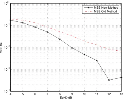
Simulation results
The simulations are made with the following parameters:
Tf = 30ns, Th = 90ns, Nf = 15, P = 3, Ns = 30. The code sequences are randomly
4 5 6 7 8 9 10 11 12 13 10−4 10−3 10−2 10−1 100 EpN0 dB MSE tau
MSE New Method MSE Old Method
Figure 4.3: MSE new method compared with the old one
channel are randomly generated. In figure we can see the MSE of the estimation of the offset (defined in (4.9)) for some values of ratio Ep
N0. The dashed curve is
related to the performance for the original algorithm. The solid curve is plotted with the same sequences but with the modification explained in this chapter. Other simulations were done, with different parameters, but similar results. The method could be improved following some more theorical criteria.
Chapter 5
Detection Theory
Detection theory is defined as how to make a decision if an event of interest is present or not [14]. In detection theory for TR-UWB Systems we want to determine whether data is present or not. This results in a binary hypothesis test, where two cases (hypotheses) are stated and the algorithm has to decide which one is (most likely) true.
In the synchronization algorithm described in chapter 3 the signal is supposed to be present starting from the first column of the data matrix built by collecting the received samples. But if the signal is not present, the data model (3.7) is not valid anymore and the synchronization algorithm doesn’t produce a correct estimation of the offset. In this chapter we propose how to detect the presence of the signal before applying the synchronization algorithm, in the single user case.
5.1
The noise samples
The mentioned model (3.7) has to be completed, because, as said in section 4.1, we must consider the presence of the noise. The assumption we make is that the noise picked up by the antenna receiver is an Additive Gaussian White Noise (AWGN).
Looking at figure 5.1 we notice now the presence of the Band Pass filter after the antenna receiver. Usually the filter is omitted. As said, we suppose Wr(t) be
AWGN, with Power Spectral Density equal to N0. The Band Pass filter keeps only
the noise in the band of the signal. Let’s suppose the signal frequency be f0 and
the radio frequency signal band be β: in figure 5.2 we can see the band pass filter frequency response.
Figure 5.1: Autocorrelation receiver with Band Pass filter
Figure 5.2: Frequency response Band Pass filter
in the figure 5.3.
Figure 5.3: Noise power spectral density
The average power of the noise W (t) is
N =
Z +∞
−∞
Sw(f )df = 2N0β (5.1)
hypothesis H0 = {T here isn0t the signal}
hypothesis H1 = {T he signal is present}
In the first case H0 the expression of Y (t) is:
Y (t) = W (t)
In the second case H1:
Y (t) = S(t) + W (t)
Under hypothesis H0 we have:
Z(t) = W (t)W (t − D) (5.2)
there is only the noise, it’s only one term. Under Hypothesis H1 we have:
Z(t) = [S(t) + W (t)][S(t − D) + W (t − D)] (5.3)
= S(t)S(t − D) + [S(t)W (t − D) + S(t − D)W (t) + W (t)W (t − D)]
there is signal plus noise, they are four terms, but three of them are noise. Then there’s the integration and the sampling. We already know the expression of the signal samples after the oversampling. What we want now is to know the statistics of the noise samples. A good analysis is made by Hoctor and Tomlinson in [13] . From this paper we can assert that in both the hypothesis H0 and H1 the noise
samples are INDEPENDENT GAUSSIAN variables, with null mean value and the same variance. Nevertheless the value of the variance is different in the two different hypothesis. In the hypothesis H0 the expression of the variance is [13]
σH20 = 4TsamN02β (5.4)
where Tsamis the integration interval and also the sampling interval. In the
hypoth-esis H1 the variance depends also on the power of the signal, in fact the expression
of the variance is σ2 H1 = 4Tsam(1 + S N)N 2 0β (5.5) where S
N is the signal to noise power ratio at the input of the pulse pair correlator
(N has the expression (5.1) ).
Now we can decide a strategy of signal detection.
5.2
The training sequence for the first stage
Considering the model (3.7), when the synchronization algorithm is applied, the signal is present starting from the first column of the matrix X. As already said:
X is a Ls× Ns data matrix and it is equal to [Cτ]h1T when the training sequence
used for the synchronization is composed of Ns+ 1 symbols all equal to 1.
So, before applying the synchronization algorithm we have to be sure that the signal is present since the first column. To do it, a good idea is to transmit a previous training sequence composed of Nd symbols still equal to 1, but with another
partic-ular characteristic: the chips of the code sequence are all equal to 1. We can define it as the ”first stage”: the detection of the presence of the signal.
Transmitting the first training sequence and collecting the samples in the same way we do in the synchronization algorithm we obtain:
X = [Cτ] h1T (5.6)
that is the same expression of (3.7) used to apply the synchronization algorithm, but in this case 1T is a N
d length vector and in Cτ the elements different by zero
are all equal to 1. Let’s think for a moment to sum all the elements of the matrix
LsXNd−1 n=0 x[k + n] = NfEhNd (5.7) where Eh = PXh−1 i=0 h[i] (5.8)
To understand it, let’s look at the following example, in which Nf = 3, P = 2,
X = [Cτ]h1T = 0 0 0 1 0 0 0 0 0 0 1 0 0 0 0 0 0 1 1 0 0 0 0 0 0 1 0 0 0 0 0 0 1 0 0 0 1 0 0 1 0 0 0 1 0 0 1 0 0 0 1 0 0 1 1 0 0 1 0 0 0 1 0 0 1 0 0 0 1 0 0 1 h(0) h(1) ... h(5) 1T X = h(3) h(4) h(5) h(0) h(1) h(2) h(0) + h(3) h(1) + h(4) h(2) + h(5) h(0) + h(3) h(1) + h(4) h(2) + h(5) 1T
If we sum the elements of each column, we obtain 3P5n=0h(n)1T or in general N
f
PPh−1
n=0 h(n)1T = NfEh1T
So that summing all the elements we obtain the expression (5.7). We’ll use this result later. Now in the next section we’ll define a criteria to set a threshold to decide if the signal is present or not.
5.3
The Neyman-Pearson theorem
Let’s start introducing a general method to detect the presence of a signal, as done also in [8].
Following [14] let’s consider to send a signal with constant amplitude A in white Gaussian noise w[n] with variance σ2. First of all, we develop the data model and
the hypothesis for this specific case. When the signal is not present we are in the ”noise only” case, the so called ”null hypothesis” , which we indicate with H0,
whereas H1 is the ”signal embedded in noise” case, the so called ”alternative
hy-pothesis”.
H0 : z[n] = w[n]
H1 : z[n] = A + w[n]
We need to define a threshold in way to decide if the received samples z[n] belong to the hypothesis H0 or H1. To do it we need to establish a certain detection criteria.
The performance of a detector can be characterized by its probability of correct detection (PD) and false alarm rate (PF A):
PF A = P robability of deciding H1 when H0 is true
PD = P robability of deciding H0 when H0 is true
It’s intuitive to understand that the two mentioned probabilities are correlated: when the probability of false alarm decreases, the probability of detection will decrease as well. We have choosen to use the Neyman-Pearson criteria: we decide a certain probability of false alarm and we maximize the probability of detection. A different approach is the Bayesian theorem: it minimizes a risk function instead of the PF A,
but requires a prior probability of the hypothesis, a so called a priori distribution, in particular it requires the probability of the signal presence, which generally is not known, as in our case. We need to have a test statistic. To do it, we start from the likelihood ratio L(z), whichis the probability of z being a data signal (hypothesis
H1 ) and the probability of z being a noise only signal (hypothesis H0), where z is
the vector composed of the samples z[n]:
L(z) = p(z; H1) p(z; H0) H1 > < H0 γ
When the samples are independent Gaussian variables we can write:
L(z) = 1 (2πσ2)N2 exp h −PN −1n=0(z[n]−A])2 2σ2 i 1 (2πσ2)N2 exp h −PNn=0(z[n])2 2σ2 i H>1 < H0 γ (5.9)
By canceling common terms and constants, this relation can be transformed to the test statistics needed to compute a threshold:
T (z) = 1 N N −1X n=0 z[n]H>1 < H0 λ (5.10)
Let’s notice that we decided to replace γ by λ, because N and σ2 are all constant
factors. What we must do now is analyze the mean value and the variance of T (z), which is our test statistic. After that we can compute the threshold:
T (z) ∈ N (0,σ
2
N) under H0 T (z) ∈ N (A,σ2
N) under H1
Following [14] , PF A and PD can be computed using the right-tail probability Q(·),
or the probability of exceeding a given value with a Gaussian distribution, as follows:
PD = Q λ − Aq σ2 N (5.11) PF A = Q λq σ2 N (5.12)
Transforming (5.12) to compute the threshold we obtain: λ = r σ2 NQ −1(P F A) (5.13)
where λ is the one threshold that yields the maximum PD for the given PF A.
5.4
Neyman-Pearson theorem to TR-UWB
The Neyman-Pearson theorem is applied to set a threshold and decide if the signal is present or not, also in the TR-UWB system we are considering in this thesis. First of all, let’s define the two hypothesis:
Hypothesis H0 : Z = N
Hypothesis H1 : Z = X + N
where X is the signal model as in (5.6) and N is the noise sample matrix. Actu-ally, the two mentioned hypothesis don’t cover the case where the signal is partially present, but we’ll take care of this case in the last section of the chapter. Following section 5.1 we know that the elements in N are Independent Gaussian Variables, with null mean value. In the hypothesis H0 the variance of each noise sample is
σ2
H0 as in (5.4), whereas in the hypothesis H1 the variance is σ 2
H1 as in (5.1). Let’s
calculate the likelihood ratio L(z):
L(z) = p(Z; H1) p(Z; H0) H1 > < H0 γ = 1 (2πσ2 H1) NdLs 2 exp · −PNdLsn=0 (z[n]−x[n])2 2σ2 H1 ¸ 1 (2πσ2 H0) NdLs 2 exp · −PNdLsn=0 (z[n])2 2σ2 H0 ¸ H>1 < H0 γ (5.14)
variables is different in the two different hypothesis. The calculation of the test statistic becomes very complex, but at the end the result is the same as (5.10):
T (z) = 1 NdLs NdXLs−1 n=0 z[n]H>1 < H0 λ (5.15)
where λ depends by both σ2
H0 , σ 2
H1 and also by NdLs. So, the test statistic coincides
with the calculation of the mean value of the matrix Z. Let’s call in general ˆµ the
calculated mean value of Z: ˆµ = 1
NdLs
PNdLs−1
n=0 z[n]. In the hypothesis H0 we define
ˆ
µH0 the test statistic:
ˆ µH0 = 1 NdLs NdXLs−1 n=0 z[k + n] = 1 NdLs NdXLs−1 n=0 n[k + n] (5.16)
whereas in the hypothesis H1:
ˆ µH1 = 1 NdLs NdXLs−1 n=0 z[n] = = 1 NdLs NdXLs−1 n=0 (x[k + n] + n[k + n]) = 1 NdLs NdXLs−1 n=0 x[k + n] + 1 NdLs NdXLs−1 n=0 n[k + n] = NfEh Ls + 1 NdLs NdXLs−1 n=0 n[k + n] (5.17)
To write (5.17) we used the result of (5.7). In both the hypothesis the test statistic is the sum of NdLs independent gaussian variable and this means that it still is
a gaussian variable. ˆµH0 is a gaussian variable with null mean value and variance
equal to σµ2 H0 = 1 NdLs σ2H0 (5.18) See figure 5.4 ˆ
Figure 5.4: Probability density function of ˆµH0 µ = NfEh Ls (5.19) and variance σ2µ H1 = 1 NdLs σH21 (5.20) See figure 5.5
Figure 5.5: Probability density function of ˆµH1
The first clarification to do is that, really, to have mean value of ˆµH1 equal to
NfEh
Ls
the detection training sequence must be composed by Nd+ 1 symbols, because in
the first column of the matrix X must be present the tail of the preceding symbol: only in that case it’s true that, in the equation (5.6), the matrix Cτ has the
struc-ture shown in figure 3.5 So let’s start finally to understand how we can detect the presence of the signal. Let’s suppose in the beginning the signal is not present. Let’s suppose that when the receiver is turned on, the user doesn’t transmit for a certain
fixed period,at least. Under this assumption we can estimate the variance of the variable ˆµH0 by estimating the variance of the noise samples applying the maximum
likelihood criteria: ˆ σ2 H0 = 1 Nl PNl
i=1n2[i], where Nldepends on how long we decide the user doesn’t
trans-mit, at least, since the receiver has been turned on. As Nl is larger, the estimation
of the variance is better. Then, we begin to collect the samples in the matrix Z and we begin to calculate the test statistic ˆµ:
ˆ µ = 1 NdLs NXdLs i=1 z[i] (5.21)
When we have the estimation of the mean value we must compare it with a threshold
λ. If ˆµ is bigger than λ we can assert that the signal is present, otherwise the signal is
not present and we must rebuild the matrix Z removing the first column and adding another column with the Ls following samples. Then we re-estimate the mean value
and we compare it with the threshold. We repeat the procedure until the estimation becomes bigger than the threshold. In that case we have detected the presence of the signal. Now we have to understand how to set the threshold λ. As we said in the preceding section, we’ll calculate the threshold under a given PF A: equation
(5.13). We already know the statistics of our decision variable in the hypothesis H0
and, applying (5.1) as we’ll show later, we know the statistics in the hypothesis H1
too. Nevertheless between these two cases there is a transition, during which the probability density function of the variable ˆµ changes from the first to the second
(from the pdf of ˆµH0 to the pdf of ˆµH1). See figure 5.6

![Figure 3.4: Code matrix C sτ X = x[k] x[k + L s ] . . . x[k + (N s − 1)L s ]...........](https://thumb-eu.123doks.com/thumbv2/123dokorg/7308100.88003/23.892.247.655.72.402/figure-code-matrix-c-sτ-x-l-l.webp)