Indice
1. Introduction ... 3
2. Presentation of the codes and data used ... 3
3. Output and evaluated physical quantities ... 6
4. Physical limits with which to compare the results ... 7
5. Results ... 9
5.1. Statistical results for the total ground deposition ... 9
5.2. Single results for the total ground deposition ... 18
5.3. Comparison of Arpege and Aladin results for the total ground deposition ... 21
5.4. Results for the time-integrated air concentration ... 24
1. Introduction
Eventhough Italy at present doesn’t have anymore on its own territory active NPPs, nonetheless it is surrounded, at less than 200 km from its borders, by several foreign NPPs, both of PWR and BWR type [1]; moreover, four national research reactors are still in operation. This situation implies for Italy the need of having provisions, experience, and capabilities to foresee in real-time the consequences over its territory of a severe accident at one of the bordering NPPs with radioactive releases to the atmosphere.
For a country with active NPPs, the previsional capabilites should be with reaction times less than about 30 minutes; for countries, like Italy, for which active NPPs are at a certain distance, the reaction times may be larger, of the order of a few hours. However, to optimize the response phase in case of an emergency, some level of anticipated preparedness should be attained, in order to have at least some ideas of the impact and its geographical distribution. To do so, in recent times a new approach has been developed for Emergency Preparedness and Response, which relies on the statistical study of the impact by simulating several hundreds (or several thousands, depending on the chosen level of details) of accidents, making recourse to real meteorological data from the past years or decades, and then making averages of the consequences. While this approach cannot give a precise answer to a real-time accident, nonetheless it is at present the most powerful one in giving indications on the type of fixed and permanent preparedness countermeasures (like number and location of radiation measurement stations, location and number of infrastructures for response, etc.) and for preparing the necessary actions for the long-term recovery phase (like preparation of sampling strategies, food ban prescritpions, decontamination procedures, etc.). The basic idea is to evaluate the consequences of a given accident at a given NPP, varying ideally the day and/or time of the accident itself and using the real atmospheric conditions of each accident time to transport in space and time the Source Term (ST).
The most advanced codes and meteorological dataset to date for these statistical studies are those developed by the French IRSN, for which FSN-SICNUC has signed a bilateral cooperation agreement in order to conduct studies for Italy. The whole study is deployed in a multi-year project; the first year, documented in this Report, is dedicated to introduce the methodology, the codes, the physical quantities evaluated by the code, the physical limits with which to compare the results for the Italian case, and the results for a first, ideal, trial case using a simplified Source Term consisting of only one isotope, namely 137Cs.
2. Presentation of the codes and data used
The code used for the calculations presented in this Report is developed by IRSN and called ldX. It is a long-range, 3D, eulerian, atmospheric dispersion code which is capable of calculating the volumetric concentration of a given isotope, averaged in an elementary cell with dimension of 10 or 50 km, depending on the spatial resolution chosen. It uses real 3D meteorological data provided over two different geographical domains:
- Arpege domain, with a 50 km spatial resolution, see Fig. 1; - Aladin domain, with a 10 km spatial resolution, see Fig. 2.
Fig. 1. Arpege domain.
Fig. 2. Aladin domain.
The meteorological data are available for ten years, between 2002 and 2011, for 600 possible emission times per year, which correspond almost to two possible emissions per day. Therefore, combining all the ten years, a total of 6000 simulations per accident are available to get the final average impact. The code is capable of taking into account the radioactive filiation and decay during transport, the wet scavenging and the dry deposition. Two possible types of ST dynamics are available:
- Puff type, which corresponds to a release concentrated in 1 hour or emission; - Unit type, which corresponds to a release concentrated in 72 hours of emission. Another parameter which can be varied is the duration of the atmospheric transport; typically this can be set, to study the impact over Italy, to 3 or 4 days.
Finally, the total emission of 137Cs must be defined; for the present study this was chosen either as 1E15 or 1E16 Bq. These two values correspond roughly to a medium ST and to a large ST; to give a reference, the total 137Cs emission from the three units at Fukushima amounted to about 2E16 Bq.
The physical model implemented in ldX is briefly described as follows; it is important to remember that eulerian models are, at present, the most advanced for the mesoscale of interest in these activities [2].
Let 𝑐𝑖 = 𝑐𝑖(𝑥, 𝑦, 𝑧, 𝑡) be the volumetric concentration in the atmosphere of isotope i; this
quantity is a scalar field defined over a given domain in R3. Its physical dimensions are [kg/m3].
Let 𝜎𝑖 = 𝑆𝑖(𝑡)𝛿(𝑥 − 𝑥𝑠, 𝑦 − 𝑦𝑠, 𝑧 − 𝑧𝑠) be a point source located in (xs,ys,zs) for isotope i. Its
physical dimensions are [kg/m3.s]. It is a mathematical representation of the ST. The mass conservation law applied to nuclide i reads
𝜕𝑐𝑖 𝜕𝑡 + 𝑑𝑖𝑣(𝒖𝑐𝑖) = 𝜎𝑖 + 𝑑𝑖𝑣 (𝜌𝑲∇⃗⃗ ( 𝑐𝑖 𝜌)) − Λ 𝑆𝑐 𝑖−Λ𝑑𝑐𝑖
which is a diffusion equation that defines mathematically the volumetric concentration field. In this equation u is the wind velocity (vector field) in (x,y,z), is the air density (scalar field) in the same point, S is the wet scavenging rate, d
is the decay constant (expressed in s-1) for isotope i and K is the air diffusivity matrix.
It is a linear, partial differential equation, with an advection term at lhs and a diffusion term at rhs. From the physical point of view it states that the removal mechanisms for isotope i from an elementary cell of the phase space (here consisting simply of R3 + time) are the spatial diffusion (due to the wind and any concentration gradients (Fick’s Law)), the radioactive decay, and the wet scavenging.
Another important removal mechanism, which is not directly implemented in the conservation equation, is the dry deposition at ground; this is included indirectly through a proper mathematical description of the boundary conditions. These are:
- ci=0 on the external boundary of the domain and at each instant, apart from on the
ground;
- because of dry deposition, at ground the following equation must be satisfied: −𝐾𝑧(∇⃗⃗ 𝑐𝑖 ∙ 𝒏)
𝑧=𝑧0 = −𝜈
𝑑𝑒𝑝𝑐
𝑖(𝑥, 𝑦, 𝑧0, 𝑡)
n being the point-by-point upward oriented normal unit vector, and 𝜈𝑑𝑒𝑝 being the dry deposition velocity for isotope i.
The diffusivity matrix K is essentially proportional to the sum of two terms: 𝑲 ∝ (𝑫 + 𝝂𝑷)
where D is the brownian diffusivity tensor and 𝝂𝑷 is the turbulent diffusivity tensor. In
pratice K results to be diagonal.
Isotope 𝝂𝒅𝒆𝒑 [cm/s]
137Cs 0.2
131I 0.5
For wet scavenging, no matter the isotope, it is:
{
Λ𝑆 = 0 𝑠𝑒 𝑅𝐻 < 𝑅𝐻𝑡
Λ𝑆 = 3.5 ∙ 10−5∙ (𝑅𝐻 − 𝑅𝐻𝑡
𝑅𝐻𝑠 − 𝑅𝐻𝑡)
RH being the relative humidity, point-by-point, with RHt a threshold value (usually 80%) and RHs the saturatio (100%) value.
The vertical component of K (Kz) is given by the s.c. Louis parametrization. The horizontal
component is taken constant and equal to 25000 m2/s (it is an areal velocity) provided the spatial resolution is set to 0.25°.
The model implemented in ldX is very similar to that of Polair3D of the Polyphemus platform, and has been validated against the European Tracer Experiment (ETEX)1, the Algeciras2 accident, and the Chernobyl accident.
3. Output and evaluated physical quantities
The output of the ldX module is in the form of an .nc (NetCDF, Network Common Data Form) file containing the concentration values at each point of the domain and at each instant for each simulation, so that 600 simulations correspond to 600 files.
For the present study it was decided to use the concentration values to evaluate two derived quantities:
- ground deposition [Bq/m2] of 137Cs cumulated at the end of the simulation;
- time-integrated air concentration [Bq.s/m3] of 137Cs, with integration time equal to the simulation time, in the lowermost calculation layer.
The ground deposition has an immediate physical meaning, and can be compared with the limits set by laws; it is logic to use the total cumulated ground deposition because this corresponds exactly to what happens in reality during an accident.
Calculating time-integrated air concentrations is not immediately of common-sense, because physically air concentrations are not retained by the elementary phase-space cells they traverse. However the health effects of these concentrations are retained by a person assumed to stay in a given elementary cell for the whole duration time of the accident (inhalation, external radiation from the radiating cloud, etc.). Therefore one can assume that the time-integrated air concentration is proportional to the expected doses.
1
https://rem.jrc.ec.europa.eu/etex/ 2
On May 30, 1998, scrap metal containing radioactive 137Cs was accidentally melted in a furnace at the Acerinox steel mill in Algeciras, Spain. 137Cs was released from the mill’s smoke stack, and spread across the western Mediterranean Sea to France and Italy and beyond.
The calculation of ground depositions and time-integrated air concentrations from the raw data contained in each .nc files is done using specific scripts realized in the Python language in a post-processing phase. During this phase also the statistical calculations are carried out, again using dedicated Python scripts, together with the production of geographical maps of the results. With this approach, one can modify the post-processing scripts according to his own needs without having to access, and eventually to modify, the ldX code sources.
4. Physical limits with which to compare the results
It might seem reductive to make calculations transporting one single isotope, 137Cs, while in reality many more are present. However one must consider that for the preliminary aims of this multi-year task, i.e. preparing a risk-based rank of the neighboring NPP sites, using only one nuclide to make comparisons is really enough; moreover, one can use typical ST information, like isotope ratios, to evaluate consequences using 137Cs as reference. In this paragraph some direct or derived physical limits are presented for Italy. ST isotopic ratios, when needed, are assumed to be those evaluated by ENEA for the Fukushima accident [4]. Another important consideration as far as response to an emergency is due for the Italian case; thanks to the fact that distance from NPPs lowers the need to take care of very fast phenomena and their associated consequences (like the administration of stable iodine pills to the population), attention is mainly to be reserved to the long-term effects of land contamination. In this regard, the Italian legislation [3] adheres to the European maximum contamination levels, the lowest ones being those related to leaf vegetables. These levels are used in this Report for the evaluation of contamination thresholds. The main contributing isotopes for leaf vegetables are reported in Tab. 1.
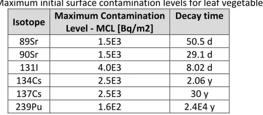
Tab. 1 Maximum initial surface contamination levels for leaf vegetables.
Isotope Maximum Contamination Level - MCL [Bq/m2] Decay time 89Sr 1.5E3 50.5 d 90Sr 1.5E3 29.1 d 131I 4.0E3 8.02 d 134Cs 2.5E3 2.06 y 137Cs 2.5E3 30 y
239Pu 1.6E2 2.4E4 y
Considering that heavy isotopes like 239Pu are not sufficiently transported over long distances, they can be disregarded in evaluating a contamination threshold for the Italian case. This threshold is defined, as usual, by the natural summation over relevant isotopes:
∑ 𝐶𝐿𝑖 𝑀𝐶𝐿𝑖
𝑁
𝑖=1
= 1
Being this a multivariate expression, recourse is to be made to isotopic ratios to reduce it to a single-parameter expression: ∑𝑋𝑖𝐶𝐿137𝐶𝑠 𝑀𝐶𝐿𝑖 𝑁 𝑖=1 = 𝐶𝐿137𝐶𝑠∑ 𝑋𝑖 𝑀𝐶𝐿𝑖 𝑁 𝑖=1 = 1
where Xi are proper isotopic ratios defined as
𝐶𝐿𝑖
𝐶𝐿137𝐶𝑠
= 𝑋𝑖 which are to be somehow evaluated.
In this way, the threshold level for 137Cs surface contamination which determines the impossibility of eating leaf vegetables due to presence of the whole mixture of isotopes (excluding 239Pu) of Tab. 1 becomes:
(𝐶𝐿137𝐶𝑠)𝐿𝑖𝑚𝑖𝑡 = 1 ∑ 𝑀𝐶𝐿𝑋𝑖 𝑖 𝑁 𝑖=1
The coefficients Xi may be evaluated, at least at first order, assuming that the transport is
the same for each isotope, and taking care of decay, as: 𝑋𝑖 ≅ 𝑆𝑇𝑖 ∙ 𝑇137𝐶𝑠∙ 𝑘𝑖 𝑆𝑇137𝐶𝑠∙ 𝑇137𝐶𝑠∙ 𝑘137𝐶𝑠 = 𝑆𝑇𝑖 𝑆𝑇137𝐶𝑠 𝑘𝑖
where 𝑇137𝐶𝑠 is a coefficient which reduces the Source Term ST because of transport (the
assumption Ti=T137Cs is made which is to be considered valid at least at first order), and 𝑘𝑖 is
another coefficient which reduces further the ST because of decay; 𝑘137𝐶𝑠 = 1 because of the very long decay time of 137Cs compared to the simulation time.
For short lived radioisotopes 𝑘𝑖 can be evaluated, again for first order estimations, using an
average time for decay for the whole simulation; this is numerically valid, in the framework of the present study, for those isotopes whose decay times are longer than about 1 day; shorter decay times would imply that the average time for decay cannot be valid for the whole domain of simulation, 𝑘𝑖 being space-dependent. For the isotopes of Tab. 1, only 131I
needs to be corrected for decay; this has about 8.02 d of decay time which, assuming 4 days of transport simulation leads to
𝑘131𝐼 ≈ 𝑒−𝜆∙4 = 0.71
In Tab. 2 the quantities needed to calculate the “equivalent 137Cs threshold level” are reported; STs are from [4] using the total over the three exploded units in the Fukushima accident.
Tab. 2 Parameters for the evaluation of the equivalent 137Cs threshold level.
Isotope MCL [Bq/m2] ST [Bq] k X
89Sr 1.5E3 4.5E16 1 2.1
90Sr 1.5E3 3.4E15 1 0.2
131I 4.0E3 2.0E17 0.71 6.8
134Cs 2.5E3 3.1E16 1 1.5
137Cs 2.5E3 2.1E16 1 1.0
With these values it is found:
(𝐶𝐿137𝐶𝑠)𝐿𝑖𝑚𝑖𝑡 ≈ 2.4E2 [Bq/m2]
Using single unit STs, this value is lowered up to about 2.2E2 Bq/m2.
For the time-integrated air concentration, it is much more difficult to propose a limiting value; this is due to the fact that many more nuclides are specified in [3] in the usual summation; many of these nuclides are not available in publicly accessible estimates of the Fukushima ST. Using only those nuclides available in [4], the limiting value of “equivalent 137Cs time-integrated air concentration” to avoid 1 mSv inhalation dose to the public would be about 2.5E7 Bq.s/m3. However, in order to take somehow into account also those nuclides not available in [4], it is decided to lower this value to 2.5E6 Bq.s/m3 which, as one might expect, is slightly conservative.
The thresholds evaluated here are used to produce the statistical analyses presented in the next paragraph.
5. Results
In this paragraph some statistical results for several parametric analyses will be presented, assuming that the emitting site is the multi-unit French site of Dampierre, about 50 km north of Orleans. Even if it is not one of the sites of direct relevance for Italy, nonetheless it is useful in assessing the capabilities of both methods and codes.
5.1.
Statistical results for the total ground deposition
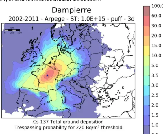
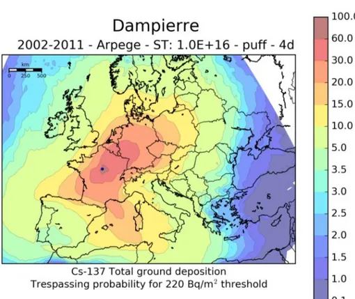
The results for the total ground deposition are presented in this section. In Fig. 3 it is shown the Arpege distribution of the trespassing probability for a threshold of 220 Bq/m2, averaged over 10 years from 2002 to 2011, with a ST of the puff type, a 3 d simulation and a total emission of 1E15 Bq 137Cs. Iso-probability levels are represented in different colors. Some general conclusions may be drawn for this emission site: a) the protective effect of the Alps can clearly be seen; b) the “barrier effect” of the Pyrenees, enhanced in the southern part and lower for the northern part, can be easily distinguished; c) the “free diffusion” towards the north, due to the absence of high obstacles, can be detected; d) the typical
effect of the “Rhone Gate”, due to the Mistral, leading to the expansion of the probability out of the Rhone valley, from the Lyon Gulf towards Sardinia, is evident. The impact over Italy can be estimated higher than threshold, with a rather uniform pattern, with a probability of occurrence between about 0.1% and 2%.
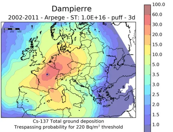
Fig. 4. Trespassing probability (%) for 220 Bq/m2, 2002-2011 years, 1E16 Bq.
In Fig. 4 it is shown the Arpege distribution of the trespassing probability for a threshold of 220 Bq/m2, averaged over 10 years from 2002 to 2011, with a ST of the puff type, a 3 d simulation and a total emission of 1E16 Bq 137Cs. The same general conclusions of the previous case can be drawn, however with different probability levels. The impact over Italy can be estimated higher than threshold, with a rather uniform pattern, with a probability of occurrence between about 3.5% (mainland) and up to a maximum of 15% (Sardinia).
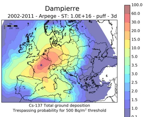
Fig. 5. Trespassing probability (%) for 500 Bq/m2, 2002-2011 years, 1E16 Bq.
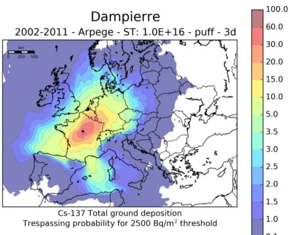
In Fig. 5 it is shown the Arpege distribution of the trespassing probability for a threshold of 500 Bq/m2, averaged over 10 years from 2002 to 2011, with a ST of the puff type, a 3 d simulation and a total emission of 1E16 Bq 137Cs. The same general conclusions of the previous cases can be drawn, however with slightly lower probability levels. The impact over Italy can be estimated higher than threshold, with a rather uniform pattern, with a probability of occurrence between a minimum of about 1.5% and a maximum of about 10%. In Fig. 6 it is shown the Arpege distribution of the trespassing probability for a threshold of 2500 Bq/m2, averaged over 10 years from 2002 to 2011, with a ST of the puff type, a 3 d simulation and a total emission of 1E16 Bq 137Cs. The distribution resembles very much that of Fig. 3 because of the linearity of the problem with respect to source and threshold (Fig. 3: ST=1E15, threshold=220 Bq/m2; Fig. 6: ST=1E16, threshold=2500 Bq/m2) and because of the very short emission time for the “puff” dynamics (1 hour).
Fig. 6. Trespassing probability (%) for 2500 Bq/m2, 2002-2011 years, 1E16 Bq.
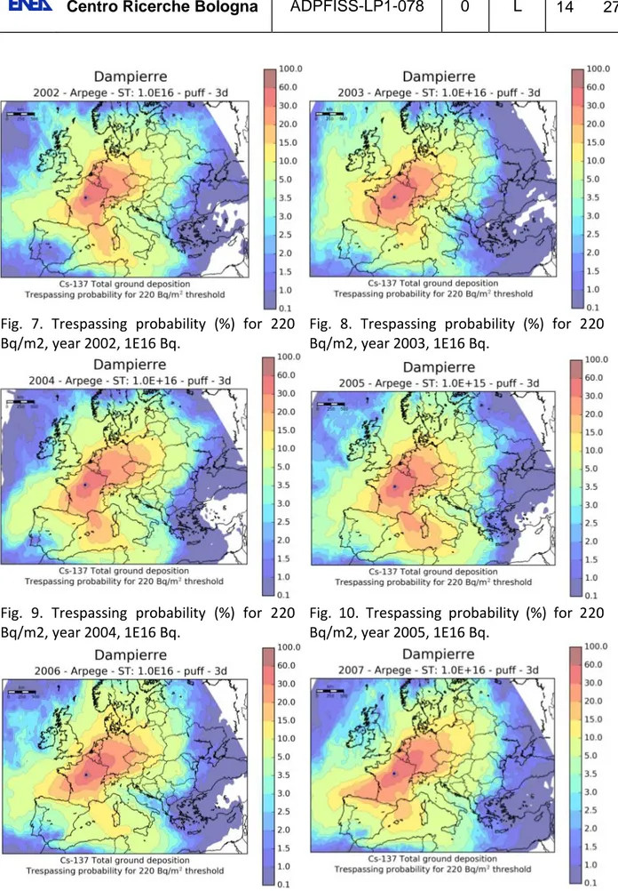
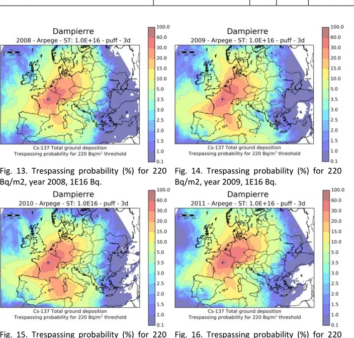
To analyze the numerical effect of the averaging procedure, it is interesting to show the distribution maps for averages made over single years between 2002 and 2011, Fig. 7 to Fig. 16. The general trend remains valid also for single-year maps; however one can notice that iso-probability curves are less smooth, due to the lower number of samples available for making the averages. Year 2010 was probably the worst for Italy, due to its peculiar weather conditions. This very same year allows to see rather distinctly the gradient effect introduced over Italy by the Apennines which decrease the probability, and hence also deposition if one assumes for valid some kind of semi-ergodic hypothesis, by a factor between 2 and 3. For 2010 the threshold trespassing probability for Sardinia was between 20% and 30%.
Fig. 7. Trespassing probability (%) for 220 Bq/m2, year 2002, 1E16 Bq.
Fig. 8. Trespassing probability (%) for 220 Bq/m2, year 2003, 1E16 Bq.
Fig. 9. Trespassing probability (%) for 220 Bq/m2, year 2004, 1E16 Bq.
Fig. 10. Trespassing probability (%) for 220 Bq/m2, year 2005, 1E16 Bq.
Fig. 11. Trespassing probability (%) for 220 Bq/m2, year 2006, 1E16 Bq.
Fig. 12. Trespassing probability (%) for 220 Bq/m2, year 2007, 1E16 Bq.
Fig. 13. Trespassing probability (%) for 220 Bq/m2, year 2008, 1E16 Bq.
Fig. 14. Trespassing probability (%) for 220 Bq/m2, year 2009, 1E16 Bq.
Fig. 15. Trespassing probability (%) for 220 Bq/m2, year 2010, 1E16 Bq.
Fig. 16. Trespassing probability (%) for 220 Bq/m2, year 2011, 1E16 Bq.
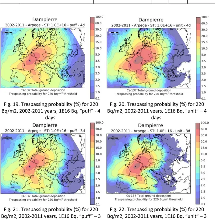
The effect of the simulation time can be estimated varying it between 3 and 4 days keeping the ST dynamics fast, i.e. of the “puff” type, so that the impact can be expected only very far from the emission site, and affecting only the periphery of the simulation (this is also more evidenced by the fact that at periphery the relative variation is higher, the absolute values being lower); any difference can therefore be ascribed to weather conditions between the 3rd and 4th day of simulation. This is detailed in Fig. 17 and Fig. 18. From this figures one can see that the areas around the emission site are almost unaffected by the simulation time whereas those rather far away are. For Italy this means an increase of about a factor 2 over Sardinia and Liguria, both affected by the “Rhone Gate” effect. It is concluded that for future studies, even if the site is nearer to Italy than Dampierre, a simulation time of 4 days is to be preferred.
Fig. 17. Same as Fig. 4.
Fig. 19. Trespassing probability (%) for 220 Bq/m2, 2002-2011 years, 1E16 Bq, “puff” - 4
days.
Fig. 20. Trespassing probability (%) for 220 Bq/m2, 2002-2011 years, 1E16 Bq, “unit” – 4
days.
Fig. 21. Trespassing probability (%) for 220 Bq/m2, 2002-2011 years, 1E16 Bq, “puff” – 3
days.
Fig. 22. Trespassing probability (%) for 220 Bq/m2, 2002-2011 years, 1E16 Bq, “unit” – 3
days.
The effect of ST dynamics, i.e. fast vs. slow, correlated with simulation time, i.e. 3 or 4 days, is shown in Figs. 19 to 22. A slower dynamics, of the “unit” type, affects mainly the areas near the emission site.
The effects of barriers and weather conditions can be seen in Fig. 23; here two barriers, the Alps, very efficient, and the Pyrenees, less efficient, represented by black lines, contribute, together with stable winds and gates, to three main principal gradients, represented by white lines, and a secondary gradient, represented by the red arc. In particular, the Alps determine the gradient toward north-east, while the Pyrenees that toward the north-west; the “Rhone Gate” and the Mistral determine the gradient toward south-east and its secondary. Using this approach one can predict the general trends of deposition for other sites around Italy.
Fig. 23. Iso-probability lines and causes of gradients for Dampierre emission site.
5.2.
Single results for the total ground deposition
To better understand how the single results may differ from the calculated average, some simulations, obtained with one single emission starting time, will be presented here. These are also useful to understand how much the level can be for the total ground deposition.
Fig. 24. 137Cs total ground deposition for an accident starting on 14 May 2002, “unit” ST.
Fig. 25. 137Cs total ground deposition for an accident starting on 14 May 2006, “puff” ST. Fig.s 24 and 25 are shown to allow a simple understanding of how different simulations can be, using the same day of different years.
Fig.s 26 and 27 are shown to see the difference between 3 or 4 days of simulation; being the dynamics of the “puff” type, as stated above, the effects and the differences appear mainly at the periphery of the domain.
Fig. 28 shows the peculiar phenomenon of “reversed” gradient for the Apennines; typically Apennines are a barrier along Italy for material transported through the “Rhone Gate”; however in this case the weather conditions are such that the material arrives from the east.
Fig. 26. 137Cs total ground deposition for an accident starting on 14 May 2002, 3 days.
Fig. 27. 137Cs total ground deposition for an accident starting on 14 May 2002, 4 days.
Fig. 28. 137Cs total ground deposition for an accident starting on 14 May 2007. Something similar, even if to a lesser extent, can be seen on Fig.s 26 and 27.
Fig.s 29 to 31 show three cases for which the impact over Italy would have been rather severe, with ample zones where the total ground deposition for 137Cs would have been beyond 1E4 Bq/m2 (Fig. 29, Campania and Calabria) or 1E3 (Fig.s 30 and 31). Fig.s 29 and 30 differ only as far as ST dynamics, the fastest one having the largest consequences.
Fig. 29. 137Cs total ground deposition for an accident starting on 14 May 2010, “puff” type.
Fig. 31. 137Cs total ground deposition for an accident starting on 14 May 2011.
5.3.
Comparison of Arpege and Aladin results for the total
ground deposition
In this paragraph a comparison of results using the two different computational domains and resolutions will be presented. In Fig. 32 the probability distribution map for 10 years over the Aladin domain is reported. Figures 33 and 34 can be used to make a direct comparison of the results from the Arpege and Aladin computational domains; both figures refer to the same set of parameters of Fig. 32 and use the same color bar. A rather good agreement is found to within one computational unit cell (it must be remembered that the value of the unit cell represents the average value within the cell itself).
Fig. 32. 137Cs total ground deposition, Aladin domain.
While the Aladin domain has an higher resolution than Arpege, it has however two drawbacks, namely that Italy is not entirely covered, and that the important Slovenian site of Krsko cannot be described being outside of the domain. One might imagine that the southern part of Italy is so far away from the northern part of Europe, where NPPs are placed, that it couldn’t be a problem if it is not included; however it is not so, because in some cases, even if rare ones, of the Dampierre emission point (which is quite far away from Italy), southern Italy can be affected (see for example Fig. 29. Therefore, unless future analyses may indicate to develop very accurate investigations of northern Italy, it is recommended to use the Arpege domain to study and classify NPPs at the national borders.
Fig. 33. Same as Fig. 32. Fig. 34. 137Cs total ground deposition: enlargement of Arpege domain result for the same case of Fig. 33.
5.4.
Results for the time-integrated air concentration
Fig. 35. Trespassing probability (%) for 2.5E6 Bqs/m3, 2002-2011 years, 1E16 Bq. Fig. 35 shows the 10 years traspassing probability map for 2.5E6 Bqs/m3 threshold; it can be seen that Italy results basically unaffected (probability < 0.1%). The time-integrated air concentration is important because it is used to evaluate dose from inhalation and direct irradiation from the radioactive cloud. Parametric analyses on the integration time (i.e. 3 or 4 days of simulation) show that the variations are mainly, as was for deposition, at the periphery of the map. However these variations are not such that Italy results affected. Fig. 36 shows the 10 years traspassing probability map but this time for 1.0E6 Bqs/m3 threshold; this was done to understand what might happen if the previous threshold of 2.5E6 Bqs/m3 had been somehow overestimated. The conclusion is that the protective effect of the Alps is so important that Italy is still unaffected (probability < 1%).
While at first sight it might seem that time-integrated air concentration is not an important parameter for future analyses, it is not so a priori, because there might be emission points, different from Dampierre, which have higher impacts; this could be the case of sites along the Rhone valley, or the site of Krsko, because of the “Bora Gate”. Be that as it may, the threshold to use in the future is probably not higher than 2.5E6 Bqs/m3.
Anyway, the rather high ST used for the time-integrated air concentration (1E16 Bq) gives a further safety margin against the reaching of the threshold.
Fig. 36. Trespassing probability (%) for 1.0E6 Bqs/m3, 2002-2011 years, 1E16 Bq.
Fig. 37. Trespassing probability (%) for 1.0E6 Bqs/m3, 2002-2011 years, 1E16 Bq, Aladin domain.
Fig. 37 reports the results for the same set of parameters of the case of Fig. 36, however for the Aladin calculation domain. The agreement is satisfactory.
Fig. 38. Time-integrated air concentration for an emission starting on 14th May 2011.
Figures 38 and 39 show two single results with emission start time on 14th May 2011 and 2010 respectively; from these maps it can be inferred that the time-integrated air-concentration is at most between 1E5 and 1E6 in the central and southern part of Italy, the main channel being, once more, the “Rhone Gate”.
6. References
[1] F. Rocchi, A. Guglielmelli, Calcoli di inventari di nocciolo: affinamento della metodologia ed applicazione ai reattori frontalieri, Technical Report ENEA ADPFISS-LP1-007, 2013.
[2] A. De Visscher, Air Dispersion Modeling: Foundations and Applications, Wiley 2013. [3] CEVAD, Emergenze nucleari e radiologiche – Manuale per le valutazioni dosimetriche e le misure ambientali, 2010.
[4] A. Guglielmelli, F. Rocchi, FAST-1, Evaluation of the Fukushima Accident Source Term through the fast-running code RASCAL 4.2: methods and results. Technical Report ENEA UTFISSM-P000-017, rev.1, 2014.