Air quality across a European hotspot
Masiol, Mauro; Squizzato, Stefania; Formenton, Gianni; Harrison, Roy; Agostinelli, A.
DOI:
10.1016/j.scitotenv.2016.10.042
License:
Creative Commons: Attribution-NonCommercial-NoDerivs (CC BY-NC-ND)
Document Version
Peer reviewed version
Citation for published version (Harvard):
Masiol, M, Squizzato, S, Formenton, G, Harrison, R & Agostinelli, A 2017, 'Air quality across a European hotspot: spatial gradients, seasonality, diurnal cycles and trends in the Veneto region, NE Italy', Science of the Total Environment, vol. 576, pp. 210-224. https://doi.org/10.1016/j.scitotenv.2016.10.042
Link to publication on Research at Birmingham portal
General rights
Unless a licence is specified above, all rights (including copyright and moral rights) in this document are retained by the authors and/or the copyright holders. The express permission of the copyright holder must be obtained for any use of this material other than for purposes permitted by law.
•Users may freely distribute the URL that is used to identify this publication.
•Users may download and/or print one copy of the publication from the University of Birmingham research portal for the purpose of private study or non-commercial research.
•User may use extracts from the document in line with the concept of ‘fair dealing’ under the Copyright, Designs and Patents Act 1988 (?) •Users may not further distribute the material nor use it for the purposes of commercial gain.
Where a licence is displayed above, please note the terms and conditions of the licence govern your use of this document. When citing, please reference the published version.
Take down policy
While the University of Birmingham exercises care and attention in making items available there are rare occasions when an item has been uploaded in error or has been deemed to be commercially or otherwise sensitive.
If you believe that this is the case for this document, please contact [email protected] providing details and we will remove access to the work immediately and investigate.
1 1 2 3 4 5
AIR QUALITY ACROSS A EUROPEAN
6
HOTSPOT: SPATIAL GRADIENTS,
7
SEASONALITY, DIURNAL CYCLES AND
8
TRENDS IN THE VENETO REGION, NE ITALY
9 10
Mauro Masiol
a,b,∗, Stefania Squizzato
a,c, Gianni
11
Formenton
d, Roy M. Harrison
b,§, Claudio Agostinelli
e12 13 14
a
Center for Air Resources Engineering and Science, Clarkson University, Box
155708, Potsdam, NY 13699-5708, United States
16b
Division of Environmental Health and Risk Management, School of
17Geography, Earth and Environmental Sciences, University of Birmingham,
18Edgbaston, Birmingham B15 2TT, United Kingdom
19c
Dipartimento Scienze Ambientali, Informatica e Statistica, Università Ca’
20Foscari Venezia, Campus Scientifico via Torino 155, 30170 Venezia, Italy
21d
Dipartimento Regionale Laboratori, Agenzia Regionale per la Prevenzione e
22Protezione Ambientale del Veneto, Via Lissa 6, 30174 Mestre, Italy
23e
Dipartimento di Matematica, Università degli Studi di Trento, via
24Sommarive 14, Povo, Trento, Italy
25
∗ To whom correspondence should be addressed.
Email: [email protected]
§ Also at: Department of Environmental Sciences / Center of Excellence in Environmental Studies, King Abdulaziz
University, PO Box 80203, Jeddah, 21589, Saudi Arabia.
2
ABSTRACT
27
The Veneto region (NE Italy) lies in the eastern part of the Po Valley, a European hotspot for air
28
pollution. Data for key air pollutants (CO, NO, NO2, O3, SO2, PM10 and PM2.5) measured over 7
29
years (2008/2014) across 43 sites in Veneto were processed to characterise their spatial and
30
temporal patterns and assess the air quality. Nitrogen oxides, PM and ozone are critical pollutants
31
frequently breaching the EC limit and target values. Intersite analysis demonstrates a widespread
32
pollution across the region and shows that primary pollutants (nitrogen oxides, CO, PM) are
33
significantly higher in cities and over the flat lands due to higher anthropogenic pressures. The
34
spatial variation of air pollutants at rural sites was then mapped to depict the gradient of background
35
pollution: nitrogen oxides are higher in the plain area due to the presence of strong diffuse
36
anthropogenic sources, while ozone increases toward the mountains probably due to the higher
37
levels of biogenic ozone-precursors and low NO emissions which are not sufficient to titrate out the
38
photochemical O3. Data-depth classification analysis revealed a poor categorization among urban,
39
traffic and industrial sites: weather and urban planning factors may cause a general homogeneity of
40
air pollution within cities driving this poor classification. Seasonal and diurnal cycles were
41
investigated: the effect of primary sources in populated areas is evident throughout the region and
42
drives similar patterns for most pollutants: road traffic appears the predominant potential source
43
shaping the daily cycles. Trend analysis of experimental data reveals a general decrease of air
44
pollution across the region, which agrees well with changes assessed by emission inventories. This
45
study provides key information on air quality across NE Italy and highlights future research needs
46
and possible developments of the regional monitoring network.
47 48
Keywords: air pollution, nitrogen oxides, particulate matter, Veneto, trends.
49 50 51 52
3
1. INTRODUCTION
53
Since the mid-90s, the European Community has adopted increasingly stringent standards for
54
abating emissions and for improving the air quality. The main steps in the legislative process were
55
the Framework Directive 96/62/EC, its subsequent daughter Directives and the more recent
56
Directive 2008/50/EC. As a consequence, a general improvement of air quality has been recorded in
57
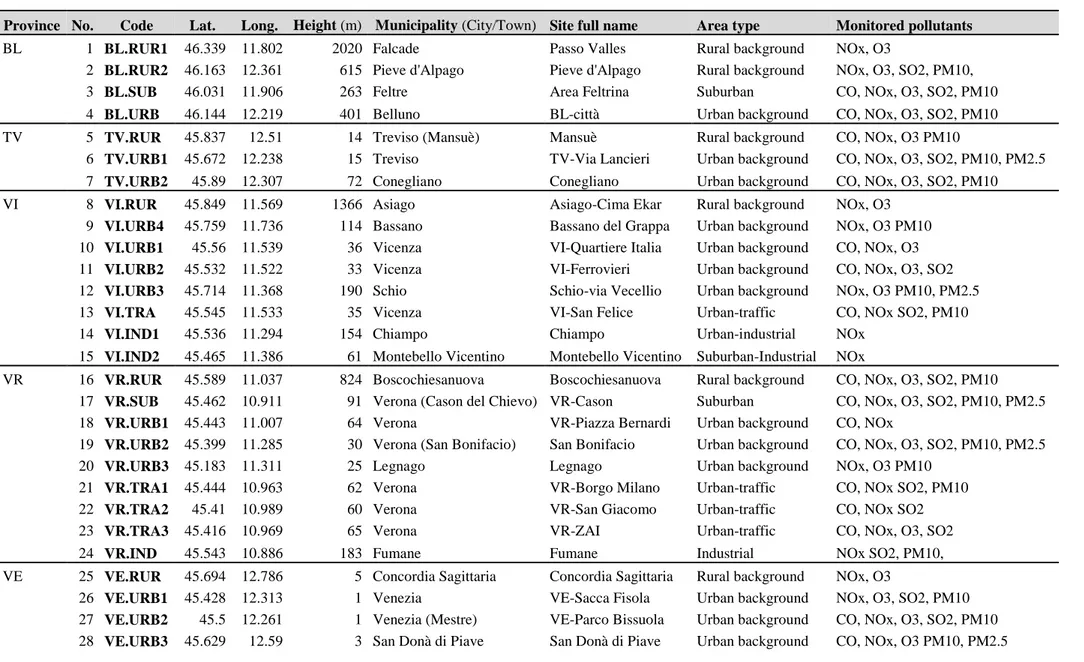
the last decade. However, current and future EU standards are still breached in some European
58
regions, the so-called hotspots, e.g., Northern Italy, Benelux and some Eastern Countries (Putaud et
59
al., 2004;2010). Under this scenario, the development of additional successful strategies for
60
emission mitigation and the implementation of measures for air quality control are two major
61
questions addressed by policy makers and in scientific research, respectively.
62 63
Following the implementation of the EC Directives, local and national authorities are required to
64
monitor air quality. Measurement data are primarily managed by local agencies to assess the extent
65
of air pollution, check if standards are complied with, and, in case of the exceeding of Limit Values
66
or even lower assessment thresholds, to inform the population about potential health impacts.
67
Beyond their original regulatory purpose, such data also represent a valuable resource: if historical
68
data are available, long-term trends can be investigated to obtain real feedback upon the successes
69
and failures of past and current mitigation strategies.
70 71
The Po Valley (N Italy) is neither a city nor an administrative unit, but it can be considered a
72
megacity (Zhu et al., 2012). Currently, it is one of the few remaining and most worrying European
73
hotspots: high levels of hazardous pollutants are commonly recorded over a wide area (~48·103
74
km2) hosting ~16 million inhabitants. The anthropogenic pressure and some peculiar
75
geomorphological features (a wide floodplain is enclosed by the Alps and Apennine mountains)
76
lead to frequently breaches of limit and target values imposed by EU Directives (EEA, 2016) for
77
nitrogen oxides, ozone and particulate matter (PM).
4 The Veneto Region (Figure 1) is located in the eastern part of the Po Valley and extends over
79
~18.4·103 km2 ranging from high mountain environments (29% of the territory), to intermediate hill
80
zones (15%), large and flat plain areas (56%) and ~95 km-long coastlines. From an administrative
81
point of view, it is subdivided in 7 Provinces: Belluno (BL), Treviso (TV), Vicenza (VI), Venice
82
(VE), Padova (PD) and Rovigo (RO). Heavy anthropogenic pressures are present almost
83
continuously: a total of ~4.9·106 inhabitants are resident in some large cities (>2·105 inhabitants:
84
Verona, Padova and Venice-Mestre) and in a number of minor towns and villages which form a
85
continuum “sprinkled” network of urban settlements. Consequently, emissions from road traffic and
86
domestic heating are spread throughout the region. Some industrial areas are also present, mainly
87
close to the main cities and with distinctive features and different plant types. In addition, the
88
Veneto lies in a strategic location linking Central, Eastern Europe and continental Italy: a dense
89
network of international E-roads and transport hubs attract large amounts of road and intermodal
90
traffic, mostly heavy duty diesel-powered trucks. A large percentage of the region includes
91
agricultural fields, mostly located in the plain (intensive farming) and hilly areas (vineyards,
92
orchards), while rural environments are present mainly in hilly and mountain regions. A land use
93
map is provided in Figure 1: this composite landscape inevitably makes the emission scenario of the
94
region extremely complex and its spatial variations quite unpredictable.
95 96
This study aims to examine and describe the spatial variations, temporal trends and seasonality of
97
air quality across the Veneto Region over 7 years (2008-2014). Datasets used in this study include
98
the mass concentration of key air pollutants as required by European air quality standards: nitrogen
99
oxides (NO+NO2=NOx), ozone (O3), carbon monoxide (CO), sulphur dioxide (SO2) and PM with
100
aerodynamic diameter less than 10 µm (PM10) and less than 2.5 µm (PM2.5). Air quality data were
101
measured by ARPAV (Veneto Environmental Protection Agency) through a well-established
102
network of 43 sampling stations (ARPAV, 2014) covering a large portion of the territory (Figure 1).
103
A series of chemometric procedures are used to assess the extent of air pollution, to verify the
5 effectiveness of site categorization and to find patterns commonly recorded across the Veneto or
105
identify sites with anomalous pollution levels. The gradients of concentrations are depicted and
106
seasonal/diurnal/weekly patterns are investigated. The long-term trends are seasonally decomposed
107
and then processed to find the general orientations and drifts in air pollution over sites with a
108
different categorization. Furthermore, long-term trends are coupled with changes in the emission
109
inventories to verify if estimated emissions match with experimentally recorded levels of key air
110
pollutants across the region.
111 112
2. MATERIALS AND METHODS
113
2.1 Sampling sites
114
The map of sites is shown in Figure 1, while Table 1 summarises their general characteristics and
115
measured pollutants. Figure 1 also shows the political, relief and land use maps. Sites are identified
116
by the initials for the province and their category. Sites were selected to fulfil some specifications:
117
(i) data availability must cover at least four years in 2008/14; (ii) sites must be representative of
118
most important pollution climate scenarios, such as citywide pollution, regional background or
119
traffic and industrial hotspots and (iii) sites must be representative of differing environments
120
(mountain, hilly, plain, coastal areas). In particular:
121
• At least one site was selected as rural background (RUR sites) for each Province (total 9 sites),
122
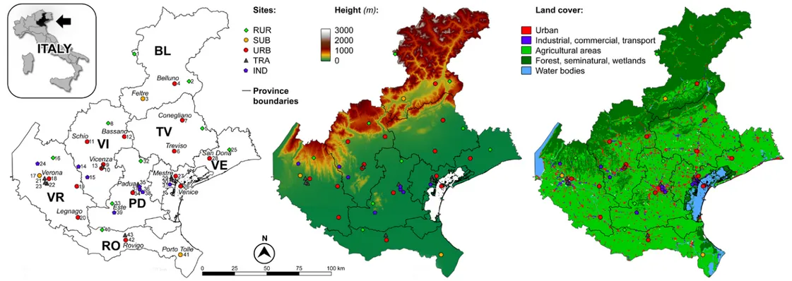
i.e. in areas not directly influenced by trafficked roads and/or urban and industrial settlements. In
123
particular, BL.RUR and VI.RUR are located in remote locations at high altitudes. RUR sites are
124
fundamental to assess the background gradients at the regional scale;
125
• Eighteen sites were categorised as suburban (SUB) and urban (URB), i.e. broadly representative
126
of citywide levels of air pollutants;
127
• A total of 8 sites were selected as representative of traffic hotspots (TRA) and placed at kerbside
128
locations in cities experiencing heavy traffic and/or frequent road congestion events;
6 • Eight sites were set as representative of main industrial (IND) areas. Each site has peculiar
130
characteristics. VE.IND is located downwind of Porto Marghera, one of the main industrial
131
zones in Italy extending over ~12 km2 and including a large number of different installations
132
(thermoelectric power plants burning coal, gas and refuse derived fuels, a large shipbuilding
133
industry, an oil-refinery, municipal solid waste incinerators and many other chemical,
134
metallurgical and glass plants). VI.IND1 and VI.IND2 are representative of small and
medium-135
sized tannery industries, PD.IND1 and PD.IND2 are set in an area potentially affected by a
136
municipal solid waste incinerator plant, PD.IND3 was selected to monitor the fall-out from a
137
steel mill and VR.IND and PD.IND4 are representative of emissions from cement plants.
138 139
2.2 Experimental
140
All selected sites are equipped with fully automatic analysers set to collect data on hourly (gaseous
141
pollutants) or hourly/bihourly bases (PM10 and PM2.5). QA/QC of measurements is guaranteed by
142
ARPAV internal protocols, which fully comply with the standards required by EC Directives
in-143
force: EN 14626:2012 for CO, EN 14211:2012 for NO, NO2, and NOx, EN 14212:2012 for SO2,
144
EN 14625:2012 for O3. CO, NOx, O3 and SO2 instruments were calibrated every day. Hourly- or
145
bihourly- resolved PM10 and PM2.5 were measured with beta gauge monitors: validation
146
experiments were routinely conducted between gravimetric (EN 14907:2005) and automatic
147
methods; several tests were also performed routinely (at least 1 test every week) to keep a constant
148
check on the beta gauge samplers. Pairs of filters were measured with both methods and the results
149
were checked to ensure that they are within the variation margins imposed by the technical
150
protocols adopted in UNI EN 12341:2001. Some sites were not equipped with hourly PMmonitors
151
(Table 1), but may provide daily gravimetric-measured PM10 levels. In this case, PM was collected
152
by low-volume samplers on filters and the mass concentration was measured by gravimetric
153
determination (EN 14907:2005) at constant temperature (20±5°C) and relative humidity (RH,
7 50±5%). Consequently, no diurnal patterns are investigated in such sites, but only interannual and
155
seasonal trends.
156 157
2.3 QA/QC and data handling
158
Data have been validated by ARPAV through a well consolidated internal protocol (ARPAV, 2014)
159
and according to the European standards. The full dataset was therefore used for exploratory
160
statistics. However, the aim of this study is to detect the general behaviour of air pollution and some
161
clearly identified high pollution episodes which occurred in 2008/14 across the region. Examples
162
are the burning of a thousand folk fires on the eve of Epiphany (Masiol et al., 2014a) or fireworks
163
for Christmas and other local celebrations. Consequently, preliminary data handling and clean-up
164
are carried out to check the datasets for robustness, outliers and anomalous records. For this
165
purpose, data greater than the 99th percentile were included for exploratory analysis but not in the
166
trend estimation. Data were also adjusted to account for the shift in anthropogenic emissions due to
167
the changes between local time (UTC+1) and daylight savings time (DST). This latter correction
168
helps in investigating daily patterns of anthropogenic emission sources.
169 170
Data were analysed using R (R Core Team, 2016) and a series of supplementary packages,
171
including ‘openair’ (Carslaw and Ropkins, 2012; Carslaw, 2015), ‘PMCMR’ (Pohlert, 2015) and
172
‘localdepth’ (Agostinelli and Romanazzi, 2011;2013).
173 174
2.4 Data depth classification analysis
175
A classification analysis was used to check the accuracy of the site categorisation, i.e., to verify
176
whether the sampling sites in a category (RUR, SUB+URB, TRA, IND) are characterised by a
177
general homogeneity in air pollutant levels. This task is accomplished by applying a new
178
classification technique based on statistical data depth (DD). This technique is well reviewed
179
elsewhere (Mosler and Polyakova, 2012 and the reference therein) and recently was extended to
8 functional and multivariate data (Ramsay and Silverman, 2006; Lopez-Pintado and Romo, 2009;
181
Lopez-Pintado and Romo, 2011; Claeskens et al., 2014; Cuevas, 2014).
182 183
The depth of a point relative to a given dataset measures how deep the point lies in the data cloud,
184
i.e. it measures the centrality of a point with respect to an empirical distribution (Mosler and
185
Polyakova, 2012). DD provides an order to the observations and the rank system provided by DD
186
can be used to perform unsupervised and supervised classification analysis. A statistical depth
187
function should be invariant to all (non-singular) affine transformations; it reaches the maximum
188
value at the centre of symmetry for symmetric distribution and it becomes negligible when the norm
189
of the point tends to infinity. Another important property is ray-monotonicity, i.e. the statistical
190
depth does not increase along any ray from the centre (Liu, 1990; Zuo and Serfling, 2000). The
191
classical notion of data depth has been extended to functional data and the different available
192
implementations aim to describe the degree of centrality of curves with respect to an underlying
193
probability distribution or a sample. Some advisable properties of functional depths are the (semi-)
194
continuity, the consistency, and the invariance under some class of transformations, which tends to
195
vanish when the norm of a curve tends to infinity (Mosler and Polyakova, 2012).
196 197
A classification analysis was performed by using the DD-plot tool and a functional multivariate
198
simplicial depth. First, a (empirical) simplicial depth of a point y with respect to a set of points x =
199
(x1, ..., xn) in the Euclidean space of dimension p is introduced. Si = S(xi1, xi2, ..., xip, xip+1) represents
200
the simplex obtained using p+1 points in the sample. A simplex of p+1 points in a space of
201
dimension p is the convex hull of those points. Then d(y; xn) is the fraction of simplicials Sn
202
contains y overall combinations of the p+1 indices i1, i2, ..., ip, ip+1 in the set 1,..., n. This is a
203
consistent estimator of the simplicial depth, which is the probability that a random simplex S(X1, X2,
204
..., Xp, Xp+1) will cover the point y when X1, X2, ..., Xp, Xp+1 are identical and independent copies of
205
the random variable X from where the sample is drawn.
9 Thus, we can consider a set of (multivariate) curves xj(t), (j=1, ..., J) measured at time t1, t2, ..., tN,
207
i.e. xj(tj) is a point in the Euclidean space of dimension p. In our context, xj(t) is the multivariate
208
time series at location j (sampling site) for a set of p pollutants concentration measured at time t.
209
Following Claeskens et al. (2014), we defined the depth of a given curve y(t) according to the
210
sample x=(x1(t), ..., xJ(t)), denoted d(y(t), x) as the weighted average of the empirical simplicial
211
depth evaluated at any given time t1, t2, ..., tN. The weights proportional to the fraction of available
212
observations at each time is then set. This is important to be considered for the presence of missing
213
values.
214 215
The classification is performed using the depth-versus-depth plot (DD-plot) (Li et al., 2012; Cuevas,
216
2014). Considering two groups of curves x=(x1(t), ..., xJ(t)) and z=(z1(t), ..., zK(t)), the goal is to
217
classify a curve y(t) in one of these. Hence, we evaluate d(y(t),x) and d(y(t),z) that represents the
218
depth of y(t) according to x and to z. We assign y(t) to the first group if d(y(t),x) > d(y(t),z) and to
219
the second group otherwise. In particular, two groups of curves will be well separated if d(xj(t),x) >
220
d(xj(t),z) for each observation xj and d(zk(t),x) < d(zk(t),z) for each observation zk. Finally, we can
221
plot on a Cartesian axis the points (d(xj(t),x), d(xj(t),z)), j=1,..., J and the points (d(zk(t),x),d(zk(t),z)),
222
k=1,..., K, i.e. the DD-plot. Curves (sampling sites) well classified in the first group will be plotted 223
at the right bottom corner of the graphics, whereas curves well classified in the second group will
224
appear at the left upper corner. Curves equally well classified in both groups will lie around the
225
bisector line of the plot.
226 227
In this study, four site categories are used to group the sites: rural (RUR), urban and sub-urban
228
(URB), traffic (TRA) and industrial (IND). For each couple of categories, the DD-plots are
229
evaluated on the basis of distributions of one or more pollutants.
230 231 232
10
3. RESULTS
233
A summary of data distributions during the whole study period (all available data) is provided as
234
boxplots in Figure 2 and maps in Figures SI1. Concentrations are expressed as mass concentration;
235
NOx is expressed as NO2, as required by EU standards. Moreover, Table SI2 reports annual average
236
concentration and exceedances for NO2, O3, PM10 and PM2.5. CO and SO2 are not included because
237
no exceedances were observed.
238 239
3.1 Carbon monoxide and sulphur dioxide
240
In Veneto, CO and SO2 are not critical pollutants. CO values are well below the EC limit value and
241
WHO guidelines (WHO, 2000), i.e. 10 mg m‒3 as daily maximum over eight hours. The highest
242
hourly average levels of CO over six years were recorded at VR.URB1, PD.IND2, VR.TRA3,
243
PD.URB, VE.TRA1 and PD.IND1 (all ~0.6 mg m‒3); remaining sites showed concentrations
244
between 0.2 and 0.6 mg m‒3.
245 246
SO2 does not show exceedances of European standards both for hourly averages (350 μg m‒3) and
247
for 24-h averages (125 μg m‒3). The 2008/14 average concentrations across Veneto were very low,
248
ranging from ~0.6 μg m‒3 (often below instrumental detection limits) at VI.URB3 and RO.SUB to
249
~4 μg m‒3 at some sites near Venice (VE.IND, VE.URB1). The higher levels in Venice sites can be
250
likely associated to harbour and industrial emissions (i.e. thermal power plant, oil refinery and
251
municipal solid waste incinerator). While the contribution of the harbour to the levels of SO2 in
252
Venice is still debated (Contini et al., 2015), the role of industrial emissions is well supported by the
253
emission inventories. In 2005, about 76% of overall SO2 emissions in the Veneto were released in
254
the Province of Venice, of which 69% (19,742 Mg y-1) came from combustion in energy and
255
transformation industries (ARPAV, 2011).
256 257 258
11 3.2 Nitrogen oxides
259
When considering the short-term metrics, NO2 does not represent a special risk for human health in
260
Veneto: the 1-hour alert threshold of 400 μg m‒3 was never breached, while the 1-hour average of
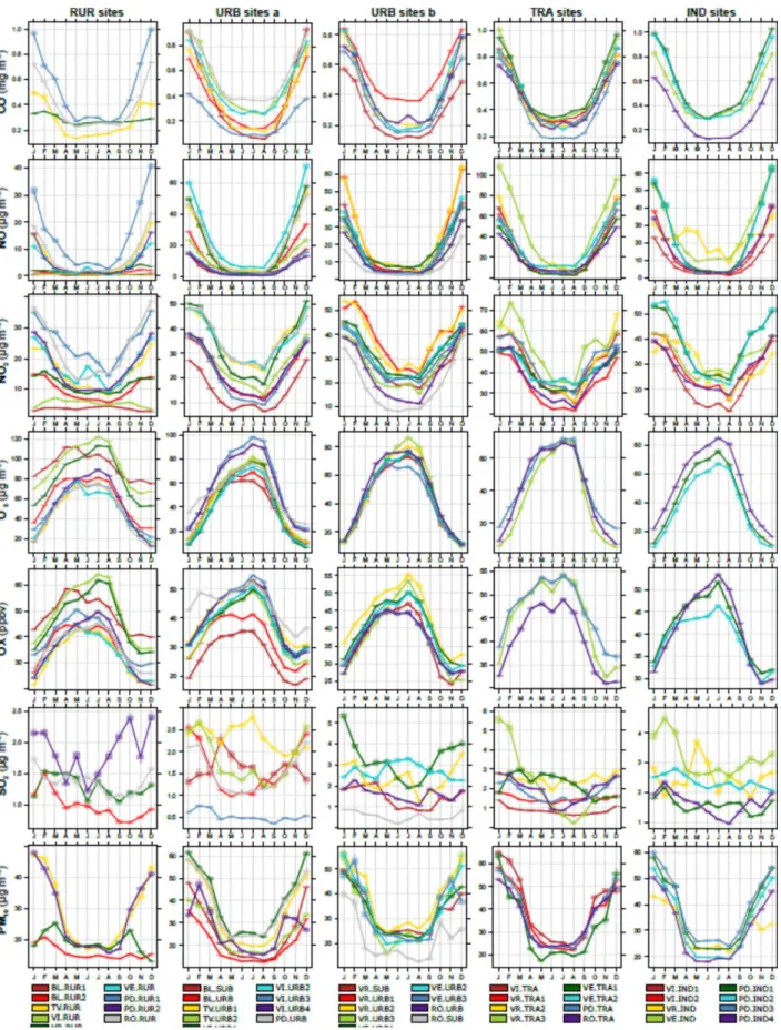
261
200 μg m‒3 not to be exceeded more than 18 times over a calendar year was exceeded only at
262
VR.TRA3 in 2008. However, NOx becomes pollutants of concern when looking at the long-term
263
metrics. The minimum average levels were found at two rural sites located in high mountain
264
environments, while maxima were measured at a traffic site in Verona located very close to a
265
logistic intermodal freight transport hub spanning over 4 km2 and moving 26 million tons of goods
266
annually (VR.TRA3). The average concentrations of NO varied from 0.5-0.6 μg m‒3 (VI.RUR,
267
BL.RUR1) to 50 μg m‒3 (VR.TRA3), while NO2ranged from 4 μg m‒3(BL.RUR1) to 53 μg m‒3
268
(VR.TRA3) and NOxfrom 5 μg m‒3(BL.RUR1) to 130 μg m‒3 (VR.TRA3). Comparing results
269
averaged over 2008/14 with the annual EC limit value for NO2(40 μg m‒3 averaged over one year),
270
the limit was substantially exceeded at six traffic sites (VE.TRA2, VE.TRA1, VI.TRA, VR.TRA2,
271 PD.TRA, VR.TRA3). 272 273 3.3 Ozone 274
In rural sites, average O3 levels ranged from 48 μg m‒3 (RO.RUR) to more than 90 μg m‒3
275
(BL.RUR1, VI.RUR), while urban and suburban sites varied between ~40 and ~60 μg m‒3. Despite
276
the low number of sites measuring ozone in traffic and industrial environments, it is evident that
277
polluted environments generally exhibit the lower average concentrations: the minimum levels were
278
recorded at VR.TRA3 (36 μg m‒3), which, inversely, shows the higher NO concentrations (it leads
279
close to a large logistic intermodal freight transport hub and, thus, it is affected by heavy traffic of
280
diesel-powered trucks).
281 282
Ozone is the subject of several regulations: the alert threshold (maximum 1-hour level of 240 μg
283
m‒3) was never breached in 2008-2012, but was exceeded five times in 2013 at PD.RUR1. This
12 result recalls the anomaly of PD.RUR1 already reported for PM10-bound polycyclic aromatic
285
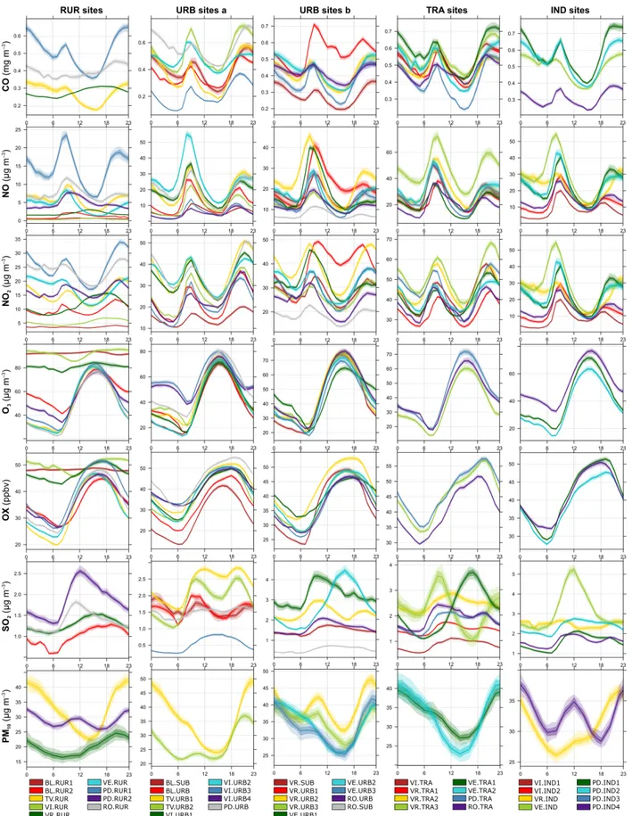
hydrocarbons (Masiol et al., 2013). Despite PD.RUR1 being originally located far from direct
286
emission sources, it probably suffers from a local unknown source of air pollution. In addition, it is
287
located between and equidistant from three main urban settlements (Mestre, Padova and Treviso).
288
Further studies should be carried out to detect the potential sources; in the meanwhile, its
289
categorisation should be revised.
290 291
The information threshold (180 μg m‒3 over one hour) was frequently exceeded at most of the sites.
292
VI.RUR deserves special attention because it is affected annually by 39‒126 exceedances; it is
293
located in a remote area (1366 m a.s.l.) characterised by grass- and wood-lands and is not affected
294
by direct anthropogenic sources. Consequently, high O3 levels may be linked to the transport of air
295
masses containing ozone or ozone-precursors from the nearby highly populated plain areas or to the
296
local biogenic emission of ozone-precursors from plants. In addition, since this area is not impacted
297
by traffic, titration of photochemically produced ozone by primary NO is negligible.
298 299
The EC long-term target value of 120 μg m‒3and the WHO air quality guideline of 100 μg m‒3
300
measured as maximum daily 8 hour running averages (not to be exceeded more than 25 days over 3
301
years for the EC target) were also frequently breached at almost all the sites. Similarly, the long
302
term objective value for the protection of vegetation (AOT40) calculated over the warm period
303
(May to July) is also amply breached at all the rural sites, posing a serious risk to high-quality
304
agriculture promoted by regional policies.
305 306
It is therefore evident that ozone is a critical pollutant across the Veneto. The standards for ozone
307
are more difficult to achieve across the warmer regions (southern Europe) because of the larger
308
magnitude of summer photochemical O3 episodes. In addition, O3 levels are also influenced
309
substantially by the extent of reactions with local NO emissions, which are currently falling in
13 Europe (Colette et al., 2011) in order to comply with the increasingly stringent emission standards
311
required for road vehicles. As a result, recent decreases in NO emissions across Europe may limit
312
reaction with O3, which is the main sink of O3 in the polluted atmosphere.
313 314
3.4 NOx partitioning and total oxidants (OX)
315
Recent changes in emission trends for some air pollutants and the complex photochemistry of the
316
NO-NO2-O3 system are further evaluated through two derived parameters. The partitioning of
317
nitrogen oxides was investigated through the NO2/NOx ratio (Figure 2 and Figure SI1b) and total
318
oxidants (OX=NO2+O3, expressed as ppb) are often used to describe the oxidative potential (Kley et
319
al., 1999; Clapp and Jenkin, 2001). Results are highly variable, but higher ratios are generally
320
recorded at rural sites because of the lower primary NO emissions. The average levels of OX show
321
little variation across the Region with distributions typically showing interquartile ranges between
322
25 and 50 ppbv. The highest site averages are seen at rural sites due to photochemical ozone
323
creation, and at traffic sites, presumably caused by high emissions of primary NO2.
324 325
3.5 Particulate matter
326
PM10 and PM2.5 are critical air pollutants in Veneto. Average PM10 levels over 2008/14 varied from
327
less than 20 μg m‒3in BL.RUR2 and VR.RUR to more than 40 μg m‒3 in VI.URB1 and VI.TRA.
328
Some sites breached the European annual limit value of 40 μg m‒3 (PD.IND3, VI.URB1, PD.URB,
329
VR.TRA2, VE.TRA1, PD.TRA and PD.IND1), except in 2013 and 2014 when no exceedances
330
were recorded. In such sites, the annual average concentrations are usually close to the European
331
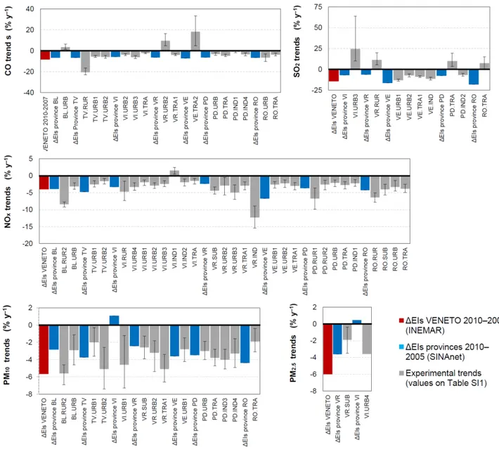
limit value: this way, small fluctuations in PM10 levels may have a large effect in marking them as
332
“fulfilling” or “not fulfilling” the EC standard.However, every year more than 20 sites exceeded
333
the daily mean of 50 µg m‒3 for more than 35 times in a calendar year. Among these sites,
334
VI.URB1, VE.TRA2, VE.IND and VE.URB3 showed the highest number of daily exceedances for
335
a minimum of 77, 66, 64 and 60 times in a calendar year, respectively.
14
337
The PM2.5 monitoring network started its operation in 2009, when the Directive 2008/50/EC entered
338
into force, and continued to grow over the following years. This way, only 8 sites provide sufficient
339
data to be included in this study. The annual limit value (25 μg m‒3) was frequently breached (five
340
years out of six) at PD.URB, PD.IND1, PD.IND2, VE.IND and VI.URB1. Similar to PM10, in 2013
341
only 6 stations breached the annual average value, while no exceedances were recorded in 2014.
342 343
4. DISCUSSION
344
4.1 Differences among sites
345
Maps showing the average levels of recorded pollutants over the 2008/14 period are reported in
346
Figures SI1a,b for different site categories. Levels of CO are generally low across the region and do
347
not show any evident trend among site categories. On the contrary, nitrogen oxides, SO2, PM10 and
348
PM2.5 show levels increasing from rural to urban to traffic sites, while concentrations in industrial
349
sites are highly variable and reflect the specific characteristics of each site (Figure 2). Such patterns
350
are opposite to ozone (higher levels at rural sites in high mountain environments and lower at sites
351
polluted with primary emissions).
352 353
Motor vehicles are major sources of NO (Keuken et al., 2012; Kurtenback et al., 2012) and a series
354
of volatile organic compounds (VOCs) (Gentner et al., 2013). Munir et al. (2012) have shown that
355
emissions from cars, buses and heavy vehicles have strong effects on urban decrements of ozone
356
levels. Due to this, the lower O3 levels in most anthropogenically affected sites in Veneto are related
357
to the primary emissions of NO. This fact is further well supported by the partitioning of nitrogen
358
oxides (Figure SI1b): lower NO2/NOx ratios are recorded at urban and hot-spot sites, indicating that
359
high relative concentrations of NO lead to ozone depletion. Another reason is linked to the impact
360
of natural sources of VOCs, such as biogenic isoprene and terpenes, i.e. known effective
ozone-361
precursors (Duane et al., 2002). The land cover map (Figure 1) shows that the hilly and mountain
15 areas of N Veneto are covered by forests. Thus, biogenic VOCs are expected to be elevated in rural
363
and mountain environments and enhance the generation of ozone. In this context, modelling studies
364
in Europe indicate that biogenically-driven O3 accounts for ~5% in the Mediterranean region (Curci
365
et al., 2009).
366 367
The Kruskal-Wallis analysis of variance by ranks (KWtest) was applied as a global non-parametric
368
test for depicting statistically significant inter-site variations. The null hypothesis is rejected for
369
p<0.05, meaning that the sites in a category are statistically different. In this case, the post-hoc test 370
after Nemenyi (Demšar, 2006) was applied for multiple sample comparison to point out the pairs of
371
sites which differ significantly in the pollutant level. Generally, results indicated that air pollutants
372
are uniformly distributed across the region: no pairs of sites differ in the levels of CO, while only
373
the two remote RUR sites (BL.RUR1 and VI.RUR) present statistically significant differences for
374
NOx and ozone from a large number of other sites. The application of comparison tests for PM10 is
375
complicated by the lack of data at the two remote sites and by the availability of differently time
376
resolved data (hourly and daily). Despite such limitations, results indicate that only BL.RUR2
377
exhibits significantly lower concentrations than other sites.
378 379
4.2 Differences amongst site categories
380
KW tests indicated that the concentrations of many pollutants measured across the Veneto are
381
statistically similar even at sites which are categorised differently (except for the two sites located
382
in extremely remote mountain areas). Moreover, the results point to an important conclusion: air
383
pollutants are almost uniformly distributed across the region. However, these results also indicate
384
that there is an apparent homogeneity amongst sites, i.e. sites having different categorisation may
385
experience statistically similar levels of air pollutants. This hypothesis was tested statistically using
386
data depth (DD) analysis. However, there are some limitations to its application: the important
387
fraction of missing data for some pollutants/sites and the lack of the full set of pollutants at most
16 sites limits the possibilities for its use. Therefore, data-depth classifications were separately
389
performed for: NO, NO2 and NOx, (ii) PM10, (iii) CO. Since few TRA and IND sites measured O3
390
and SO2, the DD analysis was not possible for these pollutants because not all the site categories
391
would be adequately represented. Application to one or a few pollutants has the disadvantage of
392
processing pollutants separately; however, it also has the advantage that it ensures the presence of a
393
reasonable high number of sites, which make the results more robust and the spatial extent of the
394
analysis more extensive.
395 396
The DD classification for nitrogen oxides (Figure 3) shows that most of RUR and URB sites are
397
generally well separated, i.e. they are plotted far from the 1:1 bisecting line. Rural sites are also well
398
separated from traffic and industrial ones. However, some exceptions are found. BL.SUB,
399
VI.URB3, VI.URB4 and RO.SUB are more similar to RUR than to URB sites, i.e. NOx levels are
400
generally lower than other urban sites, as also confirmed by boxplots in Figure 2. On the contrary,
401
PD.RUR1 and RO.RUR lie on the URB-side of the DD plot, i.e. they are more comparable to URB
402
than RUR sites. Although the anomalously high levels of air pollution at PD.RUR1 were already
403
recognised and discussed (Masiol et al., 2013), this result also shows that two rural sites probably
404
experience relatively high levels of NOx with respect to remaining RUR sites.
405 406
Although levels of pollutants in sites categorized as rural generally differ from other categories,
407
there is not a clear separation among URB, TRA and IND sites. In fact, the DD classification
408
analysis has demonstrated that most of the TRA and IND sites can be grouped with URB sites
409
(points lay around the bisector of the plot). DD-plots of PM10 also show this behaviour, while no
410
clear classification was possible using CO (Figure SI2 and SI3), i.e. CO levels are quite similar at
411
all site categories.
412 413
17 EU directives assume that URB sites are representative of the exposure of the general population,
414
while TRA and IND sites should be representative of areas where the highest concentrations may
415
occur. However, results show that this condition is rarely fulfilled in Veneto. In this context, a
416
recent position paper (JRC-AQUILA, 2013) has pointed out the need to implement criteria for
417
improving the classification and representativeness of air quality monitoring stations in Europe.
418
There are several reasons that may explain failure of the classification:
419
• The widespread distribution of emissions. Since the flat areas of the Po Valley host a ‘sprinkled’
420
continuum of urban settlements with different sizes, densities and uses (Romano and Zullo,
421
2015), the rather constant presence of anthropogenic emissions leads to a widespread distribution
422
of emission sources. As a consequence, air pollutants emitted by different sources mix in the
423
atmosphere and the limited atmospheric circulation in Po Valley further limits their dispersion.
424
• The similarity of URB and TRA sites probably results from urban planning. Most large cities
425
have ancient origins and contain medieval or even Roman city centres with historic buildings
426
and narrow streets. A rapid and intense urbanization was experienced in Italy after World War II
427
with fast build-up of large urban/suburban areas all around the ancient city centres, often without
428
a well-informed approach to urban planning. Consequently, some city configurations
429
inevitability limit the movement of road traffic and are characterised by busy streets which are
430
frequently congested during rush hour periods, i.e. when traffic is widespread over the city
431
centres and not properly channelled into main orbital or bypass roads. The high density of
432
emissions leads to a high level of pollution from road traffic across cities and to the consequent
433
similar levels of pollutants between URB and TRA sites.
434
• The poor differentiation between URB and IND sites may result from the lack of large industrial
435
zones (except in VE). Most of Veneto cities host small and medium-sized industries in several
436
sectors: glass, cement, food products, wood and furniture, leather and footwear, textiles and
437
clothing, gold jewellery, chemistry, metal-mechanics and electronics. Large industrial zones are
438
only present in VE (Porto Marghera).In addition, during the last 20 years, a large number of
18 companies have relocated their plants abroad, while the global financial crisis (2007/9) has
440
overwhelmed the industrial and economic sectors with a consequent decrease in the production
441
of goods and/or the collapse, closure or downsizing of many companies/industries. Today,
442
small/medium sized industrial areas are scattered across the region, with many of the more
443
significant industries located close to major cities. As a result, some IND sites can be more
444
affected by urban sources than industrial emissions. For example, Porto Marghera, the main
445
industrial area of Veneto, lies SE of the city of Mestre. VE.IND (representative of Porto
446
Marghera) is located just east of the industrial area (Figure SI4). During winter frequent
447
temperature inversions are responsible for the build-up of air pollutants (mostly NOx, PM) and
448
VE.IND lies just downwind of the urban area of Mestre under prevailing wind regimes (wind
449
rose in Figure SI4), while it is rarely downwind of the industrial area. Consequently, in winter
450
VE.IND is likely to be more affected by the plume from the urban area than by the industrial
451
emissions. This hypothesis is also confirmed by previous studies (Squizzato et al., 2014; Masiol
452
et al., 2012; 2014b), which reported similar concentrations of PM-bound species between
453
VE.IND and the city centre of Mestre. Further modelling studies are needed to inform
454
enhancements to the monitoring network and to better sample the industrial emissions.
455 456
4.3 Spatial gradients
457
The characteristics of anthropogenic pressures and the peculiar topography strongly influence the
458
pollutant distribution: this make the quantification of pollutant gradients very challenging. RUR
459
sites can be used as good estimators for determining gradients across the region because they can be
460
considered as representative of the regional pollution as suggested by Lenschow et al. (2001) for
461
PM: they are located away from large sources and are also fairly uniformly distributed across the
462
region. Average concentrations at RUR sites have therefore been spatially interpolated to
463
investigate the gradients of background levels of air pollutants across the region. Semi-variograms
464
were investigated, showing that all pollutants do not all have the same direction, and ordinary
19 kriging was selected as the best model to interpolate the data. In this study kriging analysis merely
466
aims to shape the background gradients because it was appliedover a limited number of points (9).
467
Maps for pollutants recorded at more than six sites (NOx, O3, OX) are provided in Figure 4, while
468
the standard errors of predictions are shown in Figure SI5. All variables show marked gradients.
469
Nitrogen oxides increase from the mountain environments in the north to the coastal plain areas;
470
however the direction of maximum slopes in the increases differ slightly: NO from NW to SE,
471
while NO2 is from NNW to SSE. The gradient for ozone is opposite to NO, with maximum
472
concentrations at high mountain rural sites and minima in coastal areas. The clear anti-correlation
473
between the gradients of NO and O3 clearly depicts their relationship: at rural sites, NO emissions
474
from anthropogenic sources are low and therefore, the reaction with ozone is its main sink, and the
475
main sink for ozone. Due to the low concentrations of NO2 at RUR sites when compared to ozone,
476
gradients for OX are similar to those of ozone.
477 478
4.4 Seasonal patterns
479
The monthly-resolved distributions of air pollutants are reported in Figure 5. No evident seasonal
480
patterns are found for the two high-mountain sites (BL.RUR1 ad VI.RUR). At the remaining sites,
481
all the pollutants except SO2 exhibit clear seasonal cycles. CO, NO, NO2, NOx, PM10 and PM2.5
482
show significantly higher levels in colder months (KWtest at p<0.05). Rapid increases occur between
483
mid-September and December; falls in concentration occur between March and mid-April. This
484
pattern can be attributed to the interplay of some covariant causes:
485
• The lower mixing layer heights in winter, which limit the dispersion of pollutants emitted
486
locally. The typical planetary boundary layer height in the Po Valley is 450 m in winter, and
487
rises up to 1500-2000 m in the warmer months due to the thermal convective activity (Di
488
Giuseppe et al., 2012; Bigi et al., 2012).
489
• Ambient temperature controls the gas-particulate phase partitioning of semivolatile compounds
490
(ammonium nitrate and part of organic carbon). In Veneto nitrate accounts for 0.1–0.5 µg m–3
20 (0.7–2.5% of PM2.5 mass) in August and for 5–10 µg m–3 (16–25%) in February (Masiol et al.,
492
2015) and organic carbon in PM2.5 varies from about 2.6 µg m–3 in June and 11.4 µg m–3 in
493
December (Khan et al., 2016).
494
• Increased emissions in the coldest months mainly driven by increasing energy demand for
495
domestic heating. Domestic heating is regulated at national level: generally, the switching on is
496
fixed to occur on 15 October, while the switching off is on15 April, i.e. when the fastest changes
497
occur. However, such dates can change according to the weather. Wood smoke from domestic
498
heating may contribute appreciably to higher winter concentrations of PM.
499
• the drop of actinic fluxes in winter and the consequent reduction of hydroxyl radical, ozone, and
500
the oxidative activity which is a sink for many pollutants.
501 502
Ozone shows a strong seasonal pattern. Ozone shows the highest values during the warmest period
503
(generally Apr–Sep), when the solar radiation is higher (Figure 5) and the atmospheric
504
photochemistry is more active. Generally, ozone levels reach approx. 20 µg m–3 in winter, but never
505
drop below 50 µg m–3 at RUR sites located in high mountain environments (BL.RUR1, VI.RUR,
506
VR.RUR >800 m above sea level). The patterns of OX are dominated by ozone both in rural and
507
polluted sites: the highest levels were reached in the rural mountain sites (BL.RUR1 2020 m asl;
508
VI.RUR 1366 m asl and VR.RUR 824 m asl).
509 510
Sulphur dioxide lacks a clear seasonal pattern. Industrial emissions are expected to be quite constant
511
through the year, but highest emissions of SO2 are may occur in summer due to an increase in
512
energy production from coal power plants to meet air conditioning demand. However, the higher
513
mixing layer height and the enhanced photochemistry driving S(IV) to S(VI) conversion lead to
514
similar concentrations to the cold period.
515 516 517
21
518
4.5 Daily and weekly patterns
519
Figure 6 reports the diurnal cycles, while Figure SI6 shows the weekly patterns. As for the seasonal
520
patterns, daily cycles are the result of interplays among the strength of sources, photochemical
521
processes and weather factors. Although minor changes due to peculiar local conditions are found,
522
almost all the sites exhibit rather similar daily and weekly cycles, except at the three high mountain
523
sites. CO and nitrogen oxides show typical daily cycles linked to road traffic at almost all the sites,
524
with two daily peaks corresponding to the morning and evening rush hours (7–9 am and 6–8 pm).
525
The morning and evening peaks are split by a minimum, which is assumed to be the result of: (i)
526
lower emissions (less traffic); (ii) larger availability of ozone driven by the daylight photolysis of
527
NOx and the oxidation of VOC and CO (iii) higher convective activity leading to a deeper mixed
528
layer, which enhances the atmospheric mixing. Weekly patterns are also linked to road traffic:
529
generally, average levels increase from Mondays to Thursdays, while a fast drop is measured during
530
weekends, when road traffic reach minimum volumes and heavy duty vehicles over 7.5 tonnes are
531
subject to some limitations (over the whole weekends in summer and on Sundays in winter).
532 533
Ozone and total oxidants (OX) show evident daily peaks in the mid-afternoon, i.e. the hours
534
experiencing the higher solar irradiation, and lower levels are experienced between 6 and 9 am local
535
time (DST time-corrected in summer). These patterns are also enhanced in summer due to the
536
higher solar irradiation. It is evident that daily peaks of OX are delayed 2-3 hours with respect to
537
ozone, corresponding to the increased NO to NO2 oxidation and primary NO2 emissions in evening
538
rush hours. The weekly patterns are the mirror images of CO and NOx with higher concentrations
539
during the weekends, following the drop of fresh anthropogenic emissions. However, such marked
540
diurnal patterns are not found at the three high mountain sites, which show rather constant and high
541
levels throughout the day. This “flatter” pattern has also been observed at other high-mountain sites
542
in the Apennines (Cristofanelli et al., 2007) and Alps (Vecchi and Valli, 1998) and is likely related
22 to the lack of anthropogenic sources of freshly emitted ozone-precursors and the presence of higher
544
levels of biogenic ozone-precursors, which do not follow anthropogenic cycling. However, the
545
levels of ozone in high mountain environments are also known to be strongly affected by (i) the
546
transport of polluted air masses by local wind systems (valley and slope winds) from the Po Valley
547
and surrounding cities inside the Alps (Kaiser et al., 2009), Foehn wind events (Seibert et al., 2000),
548
large scale synoptic air pollutant transport (Wotawa et al., 2000) and stratospheric inputs
549
(Vingarzan, 2004). Nocturnal dry deposition is also less effective at mountain sites.
550 551
Daily cycles of SO2 are quite different thorough the region and between site categories and show
552
two different patterns. Most sites present NOx-like patterns, i.e. two weak peaks corresponding to
553
the morning and evening rush hours. On the contrary, all RUR sites plus all sites in VE (with
554
different categorizations) and VI-URB3 (190 m a.s.l.) exhibited diurnal patterns very similar to
555
ozone, i.e. higher levels in the middle of the day. The two patterns remain different throughout the
556
year: different source emissions and weather factors may explain such patterns. The first cycle is
557
related to road traffic and is more evident at VR-TRA3 (close to a large logistic intermodal freight
558
transport hub), where the highest levels of NOx are recorded. In Europe, sulphur content in
559
automotive gasoline and diesel is now limited to <10 ppm (since 2009), however it is clear that
560
large volumes in traffic and congestion during rush hours may have a key effect in shaping the
561
diurnal SO2 levels. The second pattern was previously seen in Venice-Mestre (Masiol et al., 2014c)
562
and was related to local emissions from the nearby industrial zone hosting a large coal-fired power
563
plant and a large oil refinery, which are well known strong sources of SO2, as indicated by local
564
emission inventories (ISPRA, 2015; ARPAV – Regione Veneto, 2015). The closeness of VE sites
565
to the sea drives the presence of sea/land breezes (mainly in warmest periods) and has a strong
566
influence of the local circulation pattern and in bringing air masses from the industrial zone to the
567
site locations. The daytime increase in SO2 was also reported for a background site in London by
23 Bigi and Harrison (2010) who attributed it to the downward mixing of plumes from elevated point
569
sources as the boundary layer deepens during daylight hours.
570
Generally, PM10 exhibits higher concentrations overnight and clear minima in the early afternoon.
571
This pattern is consistent with the diurnal dynamics of the mixing layer. However, a secondary
572
cause may be related to the volatilisation of the more volatile aerosol compounds (e.g., nitrate)
573
during the early afternoon, i.e. when the air temperature is higher and relative humidity lower.
574
Minor peaks of PM10 concentrations can be found just before noon at a few sites affecting by very
575
different emission scenarios (VR.URB2, VR.URB3, VE.URB3, PD.RUR2, PD.IND4). Their
576
interpretation is not clear and may be related to the local characteristics of the sites.
577 578
4.6 Long-term trends
579
The long-term trends were analysed using the monthly-averaged data: since missing data can
580
significantly affect the trend analysis, only months having at least 75% of available records were
581
processed. In addition, only trends over periods extending more than 4 consecutive years were
582
computed. The quantification and the significance of the trends were evaluated by applying the
583
Theil-Sen nonparametric estimator of slope (Sen, 1968; Theil, 1992). This technique assumes linear
584
trends and is therefore useful to estimate the interannual trends, but it is irrespective of the shape of
585
trends. The slopes were also deseasonalized by using the seasonal trend decomposition using loess
586
(STL) to exclude the effect of the seasonal cycles. Details of STL are provided in Cleveland et al.
587
(1990). The statistics of the linear trends are listed in Table SI1 as percentage y‒1, while Figure SI7
588
shows all the single trends expressed in concentration y‒1 along with the upper and lower 95th
589
confidence intervals in the trends and the p-values, which indicate the statistical significance of the
590
slope estimation.
591 592
The trends observed at each site reflect both regional and local changes and are affected by the
593
particular characteristics of the site locations. However, when trends observed at individual sites are
24 aggregated at provincial or regional levels, their relationships with current and past emissions
595
inventories can be examined. The slopes calculated with the Theil-Sen method are then compared
596
with changes in primary emissions as reported in various emission inventories (EIs) available at
597
both regional and provincial level.
598 599
For each pollutant, statistically significant (p<0.05) trends expressed in percentage y‒1 are provided
600
in Figure 8 along with: (i) the differences in estimated emissions between 2010 and 2005 at
601
provincial level provided by the EI SINAnet top-down (ISPRA, 2015) and (ii) the differences
602
between 2010 and 2007/8 at regional scale provided by INEMAR (ARPAV – Regione Veneto,
603
2015). Differences of EIs (ΔEIs) are also expressed as percentage y‒1 for an easier comparison with
604
measured data (this choice considers a linear trend throughout the considered periods). Generally,
605
most of the trends are negative for all the species and the changes in measured concentrations of
606
CO, NOx, PM10, PM2.5 agree well with EIs. However, some exceptions are also found (note that not
607
all sites revealed statistically significant slopes).
608 609
CO concentrations decreased significantly at 12 of 18 sites with more than four years of available
610
data, with slopes between -20.5% y‒1 (TV.RUR) and -1% y‒1 (PD.IND1). This result is in line with
611
the average drops by -6.5% reported by INEMAR for the whole Veneto and with the EIs provided
612
by SINAnet at province scale. However, some sites show the opposite behaviour, i.e. increased
613
concentrations: BL.URB (+3.5% y‒1), VR.URB2 (+9.6% y‒1) and VE.TRA2 (+18.2% y‒1). Since
614
falls of CO in EIs are mainly driven by road transport and non-industrial combustion (including
615
biomass burning), such sites have possibly experienced local increases of road traffic volumes or
616
emissions from the use of wood for domestic heating, which is widely used in mountain areas
617
(mainly BL).
618 619
25 The average decrease of NOx levels across the whole region was estimated as -4.1% y‒1 by
620
INEMAR and was mainly attributed to “road transport” and, secondarily, to “combustion in energy
621
and transformation industry” and “combustion in industry” sectors. The average slope from data
622
measured experimentally at all the sites was -3.5% y‒1, ranging between -12.3% y‒1 (VR.IND) and
-623
1.5% y‒1 (VI.TRA). Statistically significant trends were negative at all sites except at VI.IND
624
(+1.5% y‒1). This result is a positive finding meaning that abatement strategies and improvement of
625
technologies had an effect in reducing the ambient levels of NOx. However, in recent years there
626
has been increasing interest in NOx emissions and NO/NO2 partitioning in Europe. Evident
627
discrepancies have been found between achieving NOx emission reductions and NO2 ambient
628
concentrations, which do not meet the targets in many locations (e.g., Grice et al., 2009; Cyrys et
629
al., 2012). These concerns have been related to the recent increase in NO2 levels in Europe due to
630
the increased proportion of diesel-powered vehicles, which are known to have higher primary
631
(direct) emissions of NO2 (Carslaw et al., 2007). Since the recent boom of diesel vehicles was also
632
experienced in Italy (Cames and Helmers, 2013), the relationship between significant trends of NOx
633
and NO2 needs to be further investigated.
634 635
Analysis of trends in SO2 requires particular care. Based on EIs estimations, a significant drop
(-636
14% y‒1) was experienced across the whole region, while at province level SO2 emissions decreased
637
between -18% y‒1 (in RO) and -6% y‒1 (in BL). These drops in EIs are principally attributed tothe
638
sector of combustion in energy transformation industries. In Veneto, this sector is mostly
639
represented by the energy production in coal-fired power stations, which is present in VE province
640
(Porto Marghera). In addition, the sector of ‘other mobile sources’ has also experienced significant
641
drops, particularly of ship emissions (present only in coastal areas of VE province): from January
642
2010, ships in the harbours are requested to use fuels with sulphur content <0.1%. According to the
643
EIs, experimental data show that all sites in the VE province and PD.IND2 have negative trends,
644
while four sites have experienced statistically significant increases in SO2 levels, i.e. VI.URB3
26 (+24.5% y‒1), VR.RUR (+11.4% y‒1), PD.TRA (+9.9% y‒1) and RO.TRA (+7.4% y‒1). While the
646
decline at VE sites may be attributed to the concurrent fall in industrial and maritime source
647
emissions at a local scale, the increases at other sites deserve further investigation and are possibly
648
due to long-range transport of polluted air masses. In this context, a recent study (Masiol et al.,
649
2015) has reported that Eastern Europe is a potential source area for PM2.5-bound sulphate, i.e. the
650
major sink for atmospheric SO2.
651 652
Measured data fit well with changes in EIs for PM10, except in VI province. All statistically
653
significant trends calculated from field data show decreases in PM10 concentration ranging between
654
-5.6% y‒1 in BL.RUR2 and -1.9% y‒1 in RO.TRA. PM10 emissions estimated by EIs dropped
655
between -4.4% y‒1 in RO province and -2.4% y‒1 in VR, with a slight increase in VI (+1.1% y‒1). At
656
a regional scale, the INEMAR inventory reports an overall decrease of -5.7% y‒1. Results for PM2.5
657
are quite variable, mostly due to the short series of available experimental data: only 3 sites present
658
more than 4 years of data, of which only 2 have statistically significant trends. Hence, no further
659
information can be extracted for PM2.5.
660 661
Conclusions
662
Air quality data from 43 monitoring sites have been used as input for a number of statistical tools to
663
assess the extent of air pollution across the Veneto. This paper is the first one providing information
664
from a large number of sites over a wide region of N Italy. The main findings can be summarised as
665
follows:
666
• Carbon monoxide and sulphur dioxide show low levels across the region and, therefore, are not
667
considered as critical pollutants. While CO does not show any evident spatial trend, SO2 levels
668
are higher in VE Province, particularly around Venice-Mestre. This anomaly was linked to the
669
industrial zone (coal power plant, oil refineries, other industrial installations) and harbour
670
activities;
27 • Nitrogen dioxide, ozone and particulate matter (both PM10 and PM2.5) are critical pollutants in
672
view of protecting human health, i.e. the EC limit and target values are frequently breached at
673
some sites. Those air pollutants deserve special attention because of their known adverse effects
674
upon public health: future mitigation strategies should focus on reducing concentrations of such
675
key pollutants;
676
• Air pollutants are quite uniformly distributed across the region: no pairs of sites have statistically
677
significant differences in the levels of CO, while only the two remote rural sites present
678
statistically significant differences from a large number of other sites for NOx and ozone;
679
• The current site categorization was tested by applying a data depth classification analysis: results
680
show that sites categorized as rural generally differ from other categories, while there is not a
681
clear separation among urban background, traffic and industrial sites. Probable causes of the
682
poor classification are discussed; some insights for improving the monitoring network are
683
provided;
684
• Spatial trends were investigated by interpolating average concentrations at the rural sites: despite
685
NO and NO2 having a slightly different direction of maximum slopes, nitrogen oxides generally
686
increase from the mountain to the coastal plain environments, while ozone presents maxima
687
concentrations at high mountain rural sites and minima in coastal areas;
688
• Seasonal pattern analysis revealed that CO, NO, NO2, NOx, PM10 and PM2.5 show significantly
689
higher levels in colder months and minima in summer. This pattern is mainly attributed to the
690
lower mixing layer heights, the limited oxidation potential and the emissions from domestic
691
heating. The volatilization of semi-volatile aerosol compounds during the warmer seasons is
692
another reason of this behavior for PM. On the contrary, ozone has an opposite seasonality with
693
maxima in summer due to its increased photochemical generation. No seasonal patterns are
694
found for SO2;
695
• Diurnal and weekly cycles were investigated. Generally, similar patterns are observed across the
696
region for all the measured species. A strong potential effect of road traffic emissions was found