University of Salerno
Department of Physics named after "E. R. Caianiello" and Department of Mathematics
in agreement with
University of Campania "Luigi Vanvitelli" Department of Mathematics and Physics
PhD Program:
Mathematics, Physics and Applications XXIX Cycle - 2017
Curriculum Fisica Ph.D. Thesis:
Accurate measurements of spectroscopic line parameters of atmospheric relevant molecules Candidate Tatiana A. Odintcova Tutor Coordinator
3
ACKNOWLEDGEMENTS
First of all, I would like to express my deepest gratitude to Prof. Livio Gianfrani for opportunity to join team and perform research under his guidance.
I would like to thank Dr. Antonio Castrillo, without whom it would not be possible to perform this work. I am grateful for his expert guidance, useful advices and for keeping me positive.
I would like to thank Dr. Mikhail Yu. Tretyakov for valuable discussions on the subject of the thesis.
I would like to acknowledge with gratitude Prof. Luigi Moretti, Dr. Eugenio Fasci and Dr. Maria Domenica De Vizia, Dr. Hemanth Dinesan, Dr. Pasquale Amodio for academic support and friendship.
I am grateful for the assistance given by all my colleagues and staffs, particularly Dr. Antonio Palmieri and Dr. Giuseppe Porzio.
I thank my family for love, patience and care throughout my study and all my life.
I would like to thank my friends in Italy and in Russia for their constant support.
5
Content
1. Introduction 7
2. Absorption spectroscopy: used methods and techniques 13
2.1. Beer-Lambert law 13
2.2. Line shape parameters 14
2.3. High finesse cavities 20
2.4. Optical frequency comb 23
2.5. Diode laser frequency locking 28
2.5.1. Diode laser locking to a cavity 28
2.5.2. Frequency Locking 32
2.6. Doppler Broadening Thermometry 38
3. CO2 spectroscopic parameters measurements 41
3.1. Introduction 41
3.2. Experimental setup 42
3.2.1.The optical resonator 42
3.2.2. The isothermal cell 44
3.2.3. The frequency calibration unit 47
3.3. Data analysis and results 50
3.4. Conclusion 60
4. C2H2 spectroscopic parameters measurements 61
4.1. Introduction 61
4.2. Dual-laser spectrometer at 1.39 um 63
4.3. Line shape parameters determination 67
4.4. Application to Doppler Broadening Thermometry 77
4.5. Conclusion 81
5. Concluding remarks 83
Bibliography 85
7
1. Introduction
Spectroscopy involves the interaction of electromagnetic radiation with matter. Electromagnetic radiation from microwave range to X-rays interacts with matter. Absorption spectra in different spectral ranges arise from the excitation of certain intramolecular motions. Microwave spectra correspond to molecular end-over-end rotations. Absorption spectra of infrared and visible region arise from vibration motion of the atoms. Absorption of X-rays and UV radiation is caused by transitions of electrons in atoms and molecules.
Laser spectroscopy is a reliable and powerful tool to get knowledge about matter. In particular, absorption spectra allows one to characterize the molecular structure and interaction with surrounding molecules. Specifically, measurements of the center frequency of absorption lines enable for the determination of the energy levels, lengths and angles of intramolecular bonds. From the line intensity measurements spatial charge distribution and transition probability can be obtained. From pressure broadening and shifting parameters of spectral lines, information about collision processes and intermolecular potentials can be extracted. The Doppler linewidth can be attributed to the velocity distribution of the molecules, and, consequently, to the temperature of the gaseous sample.
Besides fundamental science, accurate measurement of spectroscopic parameters is necessary for many inverse spectroscopic problems, including in particular global monitoring of atmosphere, requiring determination of concentration of major and minor constituents, such as H2O, CO2, O3, CH4, N2O, C2H2. In spite of small concentration, these
8
molecules take part in physical and chemical atmospheric processes and influence on global radiation balance.
For a proper accounting of radiation absorption and propagation in the atmosphere spectroscopic databases were created. The databases include spectroscopic parameters of atmospheric molecules, that are necessary for their spectra modeling, and for accounting radiation propagating in the atmosphere. The best known are HITRAN [1,2] and GEISA [3,4]. Every update of these databases include new and more accurate parameters of more and more transitions of larger number of molecules. High accuracy of the spectroscopic data is crucial for remote sensing because atmospheric absorption calculations assume very long traces with varying conditions, such as pressure, temperature and concentration. Thus, even small uncertainty of spectroscopic parameters leads to significant uncertainty of obtained results. Accurate experimental measurement of line intensities is much harder, than of other spectroscopic parameters. Typical uncertainties for experimental line intensity data are 3% to 10% [5-7], and even high quality measurements (e.g. [8] ) usually provide uncertainties in the 1% to 3% range.
This thesis deals with high accuracy measurements of line shape parameters of molecules of atmospheric interest, such as acetylene C2H2
and carbon dioxide CO2 including line intensity factors, pressure
broadening and shifting coefficients.
Carbon dioxide CO2 is one of principal absorbing gases of the Earth
atmosphere. Possibility to absorb radiation in the IR domain leads to significant influence of CO2 concentration on greenhouse effect, and thus,
on radiation budget of the Earth atmosphere with consequential climate change. Because of human industrial activities worldwide emission of CO2
9
increased significantly during last decades. Carbon dioxide is also prevalent in the atmospheres of some Solar system planets, such as Venus and Mars [9]. Having several absorption bands of different intensity, carbon dioxide is a good marker for probing atmospheres to different depths [10].
There are numbers of missions aimed at measurements of global concentration of CO2, as well as spatial distribution of CO2, how sources
and sinks of the carbon dioxide vary with seasons, years and locations. For instance, OCO-2 (NASA Orbiting Carbon Observatory) [11,12], GOSAT (Greenhouse Gases Observing Satellite) [10,13] and CarbonSat (preparing to launch) [14], aimed at measurements of CO2 concentration at 1 ppm
level. Absorption bands near 1.6 and 2 µm are used for CO2 concentration
measurements. Thus, uncertainty of spectroscopic parameters (specifically of line intensity) corresponding to transitions of these bands better than 0.5% is necessary, instead of it the HITRAN database provides line intensities in these bands with a relative uncertainty between 2 and 5 %. Since the last edition of the HITRAN database, there have been a large number of experimental [15, 16] and theoretical [16, 17] investigations of carbon dioxide spectra, mainly aimed at support of OCO-2 mission [11,12]. Recent ab initio calculations [16, 17] for all atmospherically important CO2
bands declares accuracy of line intensity better than 0.5 %. Before using results of these calculations they should be tested against the experimental measurements at least for a number of lines. The results of such test will be presented in this work.
Acetylene C2H2 is another minor constituent of Earth atmosphere
[18,19]. Also, it has been detected in many astrophysical objects: planets, including Mars [20], Jupiter [21], Titan [22], Uranus [23, 24], and Neptune
10
[25], comets [26], accretion disks of young stars [27], interstellar medium [28], carbon stars [29].
Production of C2H2 in the Earth’s atmosphere results from human
activities related to combustion of hydrocarbon, from fossil, bio fuels and biomass burning, and chemical industries. Its destruction occurs by reaction with OH radicals, ozone, and other oxidants. As a result, its influence on the Earth’s climate is quite significant and accurate reconstructions of vertical profiles of this trace gas are of particular relevance. Being long-life atmospheric species and having intense spectroscopic features in IR atmospheric windows C2H2 can be remotely observed. This allows to use
C2H2 as an indicator of combustion sources and as a tracer for atmospheric
transport processes and chemistry [30].
C2H2 is a linear and light molecule, thus presenting spectra with
regular rotational structure with strong isolated and well tabulated lines in the IR. C2H2 is stable gaseous species, thus easily handled. It is linked to
experimental advances in high-resolution molecular spectroscopy, as species to test. It was used to test or elaborate a variety of instrumental approach. Because of these benefits acetylene is being used as a molecular target for the spectroscopic determination of the Boltzmann constant by means of Doppler Broadening Thermometry (DBT) (see [31] and reference therein). The latter task is one of prime challenges of modern molecular spectroscopy. Fulfillment of the task requires considerable improvement of the target line shape parameters entailing achievement of an extraordinary level of experimental abilities.
In a view of aforesaid the aims of this work are:
1) Development of the new approach based on OF-CEAS technique and optical frequency comb for high accuracy CO2 line intensity measurements.
11
2) Optimization of the dual-laser spectrometer [32] and further increase of measurements accuracy of C2H2 line spectroscopic parameters. A further
aim of this thesis is the optimization of Doppler-broadening thermometry as a primary method for the spectroscopic determination of the gas temperature, for the aims of the practical realization of the new Kelvin.
Structure of the work
The basic absorption spectroscopy equations used in this work and particular experimental techniques implemented in the design of the considered spectrometers are given in the second chapter.
The third chapter is devoted to development of spectrometer operating at 2 µm and based on Optical Feedback Cavity Enhanced Absorption Spectroscopy (OF-CEAS) technique and optical frequency comb. This approach provides absolute frequency scale underneath recorded absorption spectrum. The spectrometer was used for measurements of CO2 line shape
parameters, specifically line intensities, of transitions of band 20012-00001. Unprecedented accuracy of the measured line intensity was obtained. Obtained values of measured line intensities demonstrate agreement at the subpercent level with recent most accurate to date theoretical calculations [16].
The forth chapter is dedicated to spectroscopic parameters measurements (intensity, pressure broadening and shifting coefficients) of C2H2 transition around 1.39 µm. The dual-laser approach based on optical
phase-locking was implemented. The dual laser absorption spectrometer is based on a pair of offset frequency locked lasers, one being the reference laser and the other, the probe laser, that acts as a frequency standard based
12
on noise-immune cavity-enhanced optical heterodyne molecular spectroscopy. This approach provides an absolute frequency scale underneath the absorption spectra. The spectroscopic parameters was measured with subpercent uncertainty. Application of obtained results to DBT was also considered.
13
2. Absorption spectroscopy: used methods and techniques
2.1. Beer-Lambert law
Attenuation of the laser power transmitted through the cell filled with absorbing gaseous sample is described by the Lambert-Beer law:
L e I I ( ) 0 ) ( , (2.1)
where v is frequency of the radiation, I0, I(v) are incident and transmitted
power respectively, L - absorption path length, and ()is absorption coefficient of matter per unit of length (cm-1), that is function of radiation frequency. Considering isolated resonance line corresponding to transition between ro-vibrational energy levels, the absorption coefficient can be represented as N v v g T S( ) ( ) ) ( 0 , (2.2)
where S(T) is a line strength as function of temperature (cm/molecule), v0 is
line center frequency (cm-1), g(v-v0) is normalized line shape function
(
g( 0)1) and N is a number density of the absorbers (molecules/cm3). Therefore, Lambert-Beer law can be presented in a following way:NL g T S e I I ( ) ( ) 0 0 ) ( . (2.3)
The integrated absorbance A is defined as an area under the observed spectrum over a whole spectral profile, as follows:
NL T S dv NL v v g T S dv I I A ln ( ) ( ) ( 0) ( ) 0
. (2.4)As it follows from (2.2) and (2.4), absorbance ()L is defined as
) ( )
( LAg vv0
14
2.2. Line shape parameters
The line shape profile of an isolated transition is defined by three major physical factors: natural broadening, Doppler broadening and collisional broadening. Accurate evaluation of the line shape profile requires taking into consideration the “wind” effect (the speed dependence of collisional cross-section) and Dickie narrowing (the averaging effect of velocity changing collisions).
The natural broadening of a spectral line is due to the Heisenberg uncertainty principle. Molecules can absorb radiation within a frequency range (namely, the line width), which is determined by molecular lifetime related to spontaneous transitions between a given pair of energy levels. Natural broadening results in Lorentzian line shape profile, but for ro-vibrational transitions of most atmospheric molecules at typical for atmosphere conditions influence of this mechanism is negligible in comparison with others.
The frequency of the electromagnetic radiation propagating along the y-axis, that is experienced by moving molecules, differs from the static one
v0 by the term of 0 c Vy
, where Vy - speed f molecule along y-axis,
and c - speed of light. Considering the Maxwell distribution of the speed of molecules at the thermodynamic equilibrium, one can obtain the Doppler-broadened profile, which is given by a Gaussian function:
2 0 2 ln exp 1 2 ln 2 D D D Г v v Г f , (2.6) where 0 2 ln2 M T k c v Г B
D is Doppler width (half-width at half maximum,
15
Collisions between molecules lead to changes of the quantum state of both absorbing and perturbing molecules, which leads to a reduction of the life time of the initial and final states of the transition and results in additional line broadening, called collisional broadening. Collisions may also produce pressure-dependent shifting of the transition frequency. General influence of collisions to the line shape is described by Lorentz function: 2 2 0 0 ) ( 1 ) ( Г v v Г v v fL , (2.7)
where Г - pressure broadened line width and is pressure-induced line
shift.
Doppler effect prevails at low pressures, while the effect of collisions dominates at high pressures. For intermediate pressures both effects are important. Line shape that takes into account both, Doppler and collisional broadening, is a convolution of these two profiles:
f t f t dt
fV (
,
0) D( ,
0) L(
,
0) . (2.8) This is so-called Voigt profile incorporating three parameters: Doppler width ГD, collisional width Г and shift.With improving of signal-to-noise ratio of experimental spectra up to about 1000 it becomes evident, that Voigt profile does not fit real line shape and that consideration of other fine effects is necessary. The observed lines are higher and narrower, than it follows from the Voigt profile. The deviations from the Voigt profile are attributed to the effect of collisional velocity changes (preserving the coherence with the field), which efficiently reduce Doppler width ГD , and speed dependence of the
relaxation rates, which correct the collisional profile for different velocity-classes of active molecules.
16
The effect of collision-induced velocity changes is usually known as Dicke narrowing [33]. The presence of the intermolecular collisions, which do not affect the internal state of the active molecule, and leads to velocity changes, results in reduction of the Doppler line width. The effect is usually described by the soft collision model (Galatry profile) [34] or by the hard collisions model (Rautian profile) [35].
The Galatry absorption profile was derived in the framework of the Brownian motion model [36]. The model supposes that number of collisions is necessary to change velocity of the molecule significantly. Within the Rautian model, the profile was constructed by using the method of the kinetic Boltzmann equation. The model assumes that molecular velocities before and after each collision are completely decorrelated, i.e. molecule loses completely the memory of its previous velocity and a new velocity follows Maxwell distribution.
Both models introduce one extra lineshape parameter β, optical diffusion rate, to quantify the frequency of velocity changing collisions. Previous studies [37,38] have shown that β should be smaller than the kinetic diffusion rate
MD kT
kin
, (2.9)
where M - molecular mass, D - diffusion coefficient.
The wind effect is the dependence of the collisional relaxation rate on the absolute speed of the absorbing molecule [39]. Speed dependences of the relaxation rates leads to Speed Dependent Voigt Profile. The simplest and the most common way to introduce speed dependence is quadratic approximation [40]: 2 3 1 ) ( 2 0 2 0 a a a V V Г V Г , (2.10)
17 2 3 1 ) ( 2 0 2 0 a a a V V V , (2.11)
where Г0 and 0 characterize the dependence on the active molecular
velocity Va (Va0 is the most probable value).
Both speed dependence and Dickie effects take place simultaneously. Speed Dependent Rautian Profile (SDRP) and Speed Dependent Galatry Profile (SDGP) take into account both effect. These models assume that velocity changing and rotation state changing aspects of collision are independent. But change of velocities is balanced by a change of the colliders internal states. Therefore, both velocity changing and speed dependent mechanisms operate simultaneously and their parameters are correlated.
To take into account all these effects on line shape profile the HTP profile (Hartmann-Tran Profile or partially Correlated quadratic-Speed-Dependent Hard-Collision Profile) can be used [41].
In comparison with other, more sophisticated line shape profiles (for example, SDDRGP [42]), accounting for the Dicke narrowing effect, the speed dependence of line broadening, and the partial correlation between velocity- and phase-changing collisions, the HTP can be presented in a relatively simple form and thus, rapidly computed. That is why it was recommended by IUPAC (International Union of Pure and Applied Chemistry) for using instead of the Voigt profile when high line shape description accuracy is required [43].
HTP includes 7 parameters: the Doppler width ГD, the mean
collisional relaxation rate Г0, the mean collisional shift of the line center ∆0,
the parameter accounting for the speed dependence of the collisional broadening γ2 and shifting δ2, the frequency of velocity changing collisions
18
and the parameter representing the partial correlation between velocity and rotational state changes due to collisions . Thus, the HTP profile can be expressed as follows: , ) ( ) ( 2 3 1 ) ( Re 1 ) ( 2 0 2 2 0 v B v C v A C C v v A v HTP a VC (2.12)
where A(v) and B(v) are represented by the complex probability function
w(z) )], ( ) ( [ ) ( 0 0 w iZ w iZ v v c v A a (2.13) , ) ( ) 1 ( 2 ) ( ) 1 ( 2 1 ~ ) ( 2 2 2 2 0 Z w iZ Y iZ w Z Y C v v B a (2.14) ). ( ) ( 2 2 iz erfc e dt t z e i z w z t
(2.15)In these expressions Z, X, Y, are given by the equations: , Y Y X Z , ~ ~ ) ( 2 0 0 C C v v i X (2.16) . ~ 2 2 2 0 0 C c v v Y a
where c is speed of light in vacuum and C0 , C2 and va0 are defined by , 2 3 ) 1 ( ~ 2 0 0 vVC C C C , ) 1 ( ~ 2 2 C C , 0 0 0 Г i C (2.17) ), ( 2 0 0 2 2 Г i C
19 , 2 0 M T k v B a
where va0 is the most probable speed of molecules with mass M at
temperature T, kB is Boltzmann constant. The dependence of the relaxation
rate on molecular speed va is defined by the quadratic function (2.10) as
was suggested in [39].
The HTP profile was used for analysis of the data obtained in the current work.
20
2.3. High finesse cavities
Cavity resonance can be used in absorption spectroscopy for the considerable enhancement of electromagnetic field within narrow spectral interval. High finesse optical cavities attract an interest in the field of high-sensitivity gas phase spectroscopy.
Fabry Perot resonators are composed of two spherical (or flat) mirrors with radiuses of curvature R1 and R2 parallel to each-other, facing each
other and separated by the distance L. Standing optical wave can be formed between the mirrors. Depending on the relation between R1, R2 and L, al
resonators can be divided in following configurations: plane-parallel cavity (R1=R2=∞); spherical cavity (R1=R2=L/2); hemispherical cavity (R1=∞,
R2=L); confocal cavity (R1=R2=L); convex-concave cavity (R1-R2=L).
If arbitrary beam successively reflected from both mirrors moves away from the cavity axis, the resonator is not stable. But if the beam is kept inside limited area, the resonator is stable.
Stability of laser resonators is defined by the relation of radius of curvature of two mirrors and their separation, fulfillment of the conditions is necessary to provide stable localization of light inside the cavity:
1 1 1 0 2 1 R L R L . (2.18)
Laser beams are similar to plane waves, but their intensity distributions are not uniform, they are concentrated near the axis of propagation and their phase fronts are slightly curved. Intensity distribution of laser beam is Gaussian in every cross section, width of Gaussian intensity profile changes along the axis. Considering that the Gaussian beam has its minimum diameter 2w0 at the beam waist, where the phase
21
front is plane, radius of the beam or "spot size" w(z) (the transverse distance at which the amplitude of electrical field is 1/e times that on the axis) in the plane that intersects the propagation axis at z is
2 2 0 2 0 2( ) 1 z w z w , (2.19)
and radius of curvature R(z) of wave-front that intersects the axis at z is
2 2 0 1 ) ( z z z R . (2.20)
Resonator with two plane mirrors does not support Gaussian beam. It can be coupled into spherical or hemispherical cavity. A mode of resonator is defined as self-consistent field configuration, and can be represented by a wave beam propagating back and forth between the mirrors, and the beam parameters must be the same after one complete round trip of the beam. As the beam travels in both directions between the mirrors it forms the axial standing wave pattern that is expected for a resonator mode [44]. During each round trip, a portion of light leaks out through the cavity mirrors at a rate proportional to the intracavity losses.
22
As it is shown in Fig. 2.3.1. transmission of the cavity is represented by comb of resonances (eigen modes of the cavity) equally spaced by free spectral range
L c FSR
2
. Transmitted intensity is given by the well-known Airy formula: 2 sin 1 2 1 1 ) 1 ( ) ( 2 2 2 2 r in out t R R R T I I , (2.21) 2 1r r R , T t1t2 ,
where t, r - field transmission and reflection coefficient of the two cavity mirrors. Around a resonant frequency the transmitted intensity given by eq. (2.21) is well approximated by a Lorentzian function. Full width at half maximum (FWHM) of this resonance is
R R t v r 1 1 . Width of the
resonances and cavity FSR define cavity finesse and Q-factor:
R R v FSR F 1 , (2.22) F FSR v Q , (2.23)
where v - optical frequency of excitation. The higher reflectivity of the mirrors, the narrower the cavity modes, and higher cavity finesse. It is worth to mention, that resonances of high-finesse cavity can be spectrally narrower than the laser. Ring down time RD or the photon lifetime in the
cavity is defined by the cavity resonance widthv:
R R c L R R v RD 1 1 1 . (2.24)
23
2.4. Optical frequency comb
Since the optical frequency comb has been invented [45,46] it found applications in laser spectroscopy as an optical ruler. Knowing frequencies of the comb teeth one can find frequency of the laser by measurements of the beat note between unknown laser frequency and the comb component frequency. An optical frequency comb consists of lines separated with equal distance in frequency domain and it stretches through up to about an octave. The frequency comb can be obtained by stabilization of the femtosecond pulse train generated by a mode-locked laser. The first demonstration of self-referenced frequency comb generation relied on mode-locked Ti: sapphire lasers [47]. More recently, optical frequency comb generators based on fiber lasers (for example erbium-doped fiber lasers) have also been developed [48]. Fiber sources have the potential for a more practical, robust and compact setup, as required for real-world applications. Frequency comb laser sources are commercially available from different producers.
As it is shown in Fig. 2.4.1 typical fiber laser-based frequency comb system consists of a mode-locked laser oscillator, amplification and a spectral broadening part, a detection unit and control electronics, that stabilize frequencies of the comb lines.
Mode-locked lasers emit a periodic train of femtosecond optical pulses. Electric field of the mode-locked laser pulse, circulating in the laser resonator, can be represented as product of pulse envelope function e(t) and continuous wave with carrier frequencyc:
t i c e t e t E( ) ( ) . (2.25)
24
Pulse electric field over time is shown in upper panel of Fig. 2.4.2. In the figure ceo - carrier envelope phase - is the shift between the peak of the envelope and the closest peak of carrier wave.
Fig. 2.4.1. Simplified diagram of a typical fiber laser-based frequency comb system. The pulsed output of a fiber laser oscillator is amplified and spectrally broadened. These pulses are then launched into highly nonlinear fiber in which nonlinear processes such as self-phase modulation, self-steepening, four-wave mixing, and Raman scattering spectrally broaden the pulses up to about full octave. The detected signals are used in a control loop for stabilization.
Power spectrum of identical pulses train having any shape and separated by a fixed interval can be obtained by a Fourier series expansion, translating the amplitudes from the time domain to the frequency domain. It results in a comb of regular spaced frequencies, where the comb spacing is defined by the time between pulses, i.e. it is the repetition rate frep of the
laser that is producing the pulses.
Difference between the phase and group velocities inside the cavity for the train of pulses emitted by a mode-locked laser leads to the pulse to pulse change of phase ceo arises, that is defined as
25 c c p g ceo l 1 1 , (2.26)
where lc round trip length of the cavity, c is "carrier" frequency.
Considering that ceo is evolving with time, such that from pulse to pulse there is phase increment of ceo, in the spectral domain shift of line frequencies comes around:
ceo rep ceo f T f 2 1 2 1 0 . (2.27)
The optical frequencies fn of the comb lines are fn nfrep f0, where n is a large integer (of the order of 106) that indicates the comb line, f is the 0
offset due to the pulse-to-pulse phase shift, frepis the repetition rate frequency. The mode-locked laser emits a spectrally narrow and unstable frequency comb. Then, the pulses are amplified and narrowed, so that the spectral broadening section provides the comb covering slightly more than full optical octave. At this point, optical frequency of each comb tooth is not known and not stabilized. The correspondence of time- and freq- domain pictures is presented in Fig. 2.4.2.
The frequency of repetition rate and cavity envelope offset frequency must be stabilized upon frequency standard for absolute frequency measurements. The repetition rate frequency is detected by the fast photodetector (FPD). A servo loop controls the repetition rate of the laser by comparing the FPD signal with a radio frequency (RF) standard. For optical frequency comb generator with the optical spectrum span of an octave in frequency, cavity envelope offset frequency can be obtained applying interferometric measurement. The second harmonic crystal is used to produce doubled in frequency comb lines of the low frequency portion of the spectrum. They will have very close frequencies with the comb lines
26
on the high frequency side of the spectrum with index 2n. The beat note between these lines corresponds to the offset frequency
0 0 0
2 2( ) (2 )
2fn f n nfrep f nfrep f f . A servo loop controls the offset frequency of the laser by comparing the FPD signal to a frequency standard. frep and f0are controlled by cavity length and pump power respectively.
Fig. 2.4.2. Optical pulse train and spectrum emitted by a mode-locked laser. a) The carrier wave (red) and the pulse envelope (blue) travel with different phase and group velocities, leading to a carrier-envelope phase shift. b) The optical spectrum of a mode-locked laser consists of frequency teeth separated by the repetition rate of the laser. The standard method of detecting fceo with f-2f interferometer is shown.
In the case when frep and f0 are stabilized, and thus, all frequencies of
the comb teeth are known, any optical frequency within the range of the frequency comb can be determined by recording a beat note between the unknown frequency and the comb tooth. The frequency of the laser fDL can
27
be found as fDL=fnfbeat, where fbeat is frequency offset (or beat note)
28
2.5. Diode laser frequency locking
High accuracy absorption spectroscopy requires not only absolute and linear frequency scale but also a highly monochromatic source of a probe radiation. Diode laser (DL) has short (µs) coherence time, thus average frequency dispersion (laser spectrum) with FWHM of more than 1 MHz. Growing need of lasers with high spectral purity has stimulated the development of a number of DL frequency stabilization techniques. These techniques are based on: optical feedback (OF) [49], external cavities [50], injection locking [51] and electronic servo control [52]. Because of the spectral characteristics of the diode laser frequency noise, the only systems that are able to achieve substantial linewidth reduction are those that incorporate OF or use very fast electronic servos (with bandwidth more than 20 MHz). In the following two paragraphs these two approaches are described.
2.5.1. Diode laser locking to a cavity
The high sensitivity of the diode lasers to OF is a well-known phenomenon that generally has a disruptive effect on the lasers output frequency and amplitude stability [53]. The sensitivity to OF can be put to advantageous use. The DL coherence may be increased when frequency selected optical field originating from a mode of a high finesse cavity is re-injected into DL. Fabry-Perot cavity can serve as an optical feedback element that forces a diode laser automatically to lock its frequency optically to the cavity resonance. With the appropriate optical geometry the laser optically self locks to the resonance of Fabry-Perot cavity. The
29
method relies on having optical feedback occur only at the resonance of high finesse cavity.
A feature of the laser locking system [54] represented in Fig. 2.5.1.1 is that there is an optical feedback to the laser only when its frequency matches the resonant frequency of the reference cavity. Confocal cavity in off axis operation is simple and effective configuration for this purpose. The output beam labeled as I is a combination of the reflected from the input mirror beam and resonant field inside the cavity. This beam has a power minimum when the laser frequency matches a cavity resonance. The outputs labeled as II contain only the transmitted cavity resonant field. When the DL frequency does not match to cavity resonance there is no optical feedback and laser frequency scans as usual with changes in the injection current. As the DL frequency approaches a cavity resonance, resonant feedback occur and the DL frequency locks to the cavity resonance, even if the laser current continues to scan [54].
Fig. 2.5.1.1. Schematic the optical feedback locking system [54].
New approach incorporating OF, namely OF-CEAS (Optical Feedback Cavity Enhanced Absorption Spectroscopy) was developed in work [55] for fast and accurate trace gas measurements. Locking to a cavity
30
with V-geometry with much higher cavity finesse in comparison with confocal cavity was used in [54]. Similar system operating around 2 µm was developed by the authors of the work [56].
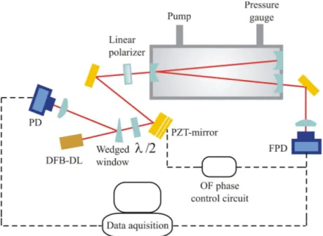
The setup consists of a distributed-feedback diode laser (DFB-DL) coupled to the high-finesse (~105) optical cavity. This latter is mounted in a “V” shape configuration by using three high-reflectivity mirrors (Fig. 2.5.1.2). The idea of the technique is that cavity provides selective optical feedback to the DFB-DL from the intracavity field when the laser frequency coincides with that of one of the cavity modes.
Laser radiation having stable amplitude and large spectral width is injected into the cavity through the folding mirror. Transmitted light possesses a very low spectral width, given by the cavity mode width, but a high level of amplitude fluctuations. When returning part of this radiation into the laser, the saturated gain dynamics dampens those fluctuations. In addition, OF acts as injection seeding at the cavity resonance frequency. Since a DL is a good, low-coherence, broad-band amplifier, injection seeding results in driving the laser field highly monochromatic. Light finally emitted from the laser-cavity loop has stable amplitude with a long coherence time [55]. Such OF with optimized parameters results in substantial reduction of the laser linewidth. For example, for the setup described in [56] in free running conditions the width is about 2 MHz, the action of the OF results in a narrowing of the linewidth to the level of 10 kHz, which is even less than the cavity mode width. This narrow band radiation is frequency locked to one of the cavity mode.
Important parameters for an efficient OF-locking are represented by the feedback rate (that is ratio of the power of light coming back from the cavity to the laser to laser power) and the distance between the laser and
31
the optical cavity, which determines the phase of the light coming back to the laser [55]. The feedback rate can be regulated by a proper combination of a half-wave plate and a polarizer and constitutes about 10-5. As was shown in [55], optimal laser-to-cavity distance should be about the length of the V-cavity arm. When scanning the laser over successive cavity modes, the wavelength change affects the number of oscillations of the laser field on its way to and from the cavity giving different OF phase. This shifts the locking interval over the resonance profile. The distance can be adjusted in a real time by a mirror mounted on a piezo actuator actively controlled by electronic feedback circuit. Cavity output is monitored by fast 1.5-MHz bandwidth InGaAs photodetector during frequency scan. The feedback circuit employs symmetry of monitored cavity modes to produce an error signal for mirror piezo adjustments.
Fig. 2.5.1.2. Sketch of the radiation source of the spectrometer. DFB-DL distributed-feedback diode laser, PD - photodetector, FPD - fast photodetector, /2 - half wave plate.
32
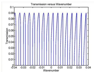
Fig. 2.5.1.3. Transmission signal of the V-cavity.
Locked laser frequency jumps from one resonance to another very quickly passing through the free running condition supplying the stepwise scan. Frequency of the laser is tuned by sweeping its driving current. High quality of radiation on both vertical (intensity) and horizontal (frequency) scales is crucial for high precision measurements. Spectral data points are taken at the frequency comb of the equidistant TEM00 cavity modes, which
do not move during short time of the laser scan. OF enables injection efficiency orders of magnitude better than without feedback. Thus the setup provides, at the output cavity mirrors, a stable and equally spaced comb-like radiation structure (Fig. 2.5.1.3) in which the frequency distance between two consecutive teeth is determined by the cavity free-spectral range (FSR).
2.5.2. Frequency Locking
Frequency control of the laser can be accomplished by stabilizing its frequency relative to a stable reference (such as another independently stabilized laser), at a precise frequency difference, which is referenced as a frequency locking. Frequency locking allows precise control, stabilization
33
and synchronization of the probe laser frequency. Frequency locking can be realized by means of optical phase-locking loop (OPLL) or offset frequency locking (OFL).
A first step in both OPLL and OFL requires to detect the beat-note signal between the two lasers using a fast photo-detector. Then (see Fig. 2.5.2.1) the radio frequency beat-note signal is amplified and subsequently scaled in frequency by a factor of N using a divider. Obtained signal is sent to a phase and frequency detector (PSD), which compares it to a reference signal provided by a RF synthesizer thus producing an error signal proportional to the difference of phases between reference and beat-note signals. After, the error signal is properly integrated (providing strong response to slow deviations and moderate response to the fast deviations) and used to continuously lock the frequency of the beat note with frequency of the reference signal. For this purpose, servo system is used. Servo system provides correction signal, that is applied to the laser frequency control electronics. The system allows to actively control the laser emission frequency in such a way that frequency offset between probe laser and reference laser is forced to maintain frequency fRF set by RF
synthesizer. The stabilized frequency of the probe laser fDL is defined by RF frequency fRF and frequency of the optical reference fref :
RF ref
DL f N f
f . Once the frequency locking loop is activated highly accurate frequency scan of the probe laser frequency can be performed by tuning the RF frequency.
Providing phase coherence between the two lasers, OPLL allows to transfer a long term stability of the reference frequency standard to any frequency of the range under consideration. OPLL represents servosystem, in which phase of the signal under control is adjusted to the phase of high
34
stable reference signal. A broad bandwidth of the overall control loop electronics is required in this approach to ensure that the optical sources are accurately synchronized, which makes this technique to be very complicated. In many spectroscopic experiments phase coherency is not required and it is sufficient that the probe laser maintains precisely fixed frequency-offset from a reference laser. In this case the control bandwidth can be rather narrow and OFL can be implemented as simpler (one control channel) locking scheme, still ensuring high frequency stability of the radiation.
Fig. 2.5.2.1. Scheme of (A) Optical phase-locking loop (OPLL); (B) offset frequency locking (OFL).
Two setups implementing frequency locking were used in the current work. The first scheme was used to control frequency of the external-cavity diode laser (ECDL) working at 1.39 µm. As optical reference an optical frequency standard based on noise-immune cavity-enhanced optical heterodyne molecular spectroscopy (NICE-OHMS) [57] was used. The emission frequency of the second ECDL (serving as a reference laser (RL))
35
was actively stabilized against the center of a sub-doppler H218O line
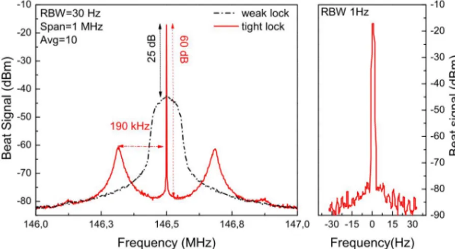
profile, observed under optical saturation conditions in a high-finesse resonator [57]. NICE-OHMS provides a dispersion signal which is employed as an error signal. The emission line width of the RL was carefully determined from measurements of the radiation noise power spectral density at different frequency offsets. The linewidth of the optical frequency standard is about 7 kHz (full width at half maximum) for an observation time of 1 ms [58]. The probe laser (PL) was phase locked to the reference laser by using the broadband phase-locking electronics that is shown in Fig. 2.5.2.1.(A). More specifically, portions of the two laser beams are focused on a fast photodetector (with a bandwidth of 12 GHz) to produce a beat-note signal which is sent to a power amplifier (model RF BAY LPA-8-17), scaled down in frequency by a factor of 40 (by using a frequency divider, model RF BAY FPS-40-12), split into two parts and then sent to a pair of digital phase and frequency detectors. The first one (PSD1, model RF BAY PDF-100) has an integrated loop filter limiting its bandwidth to 10 kHz, while the second (PSD2, model Analog Devices 9901) is much faster. The first PSD ensured a robust and reliable frequency lock in the audio bandwidth (roughly 1 kHz for the loop controlling the extended cavity length and 10 kHz for that acting on the laser current through its driver), whereas PSD2 ensured an effective phase locking between the two lasers directly controlling the diode laser current. A radio-frequency synthesizer (model RHODE&SCHWARZ SMBV100) provides the reference RF signal for both the PSDs, determining the tunable offset frequency between the two lasers. As a result of the action of the third loop, a significant narrowing (down to the Hz level) of the beat-note could be observed (Fig. 2.5.2.2, right). This demonstrates that the PL spectral purity
36
could be improved up to the limit determined by the RL. The efficient control bandwidth was estimated from the servo bumps that appear in the spectral shape of the closed-loop beat-note signal (Fig. 2.5.2.2, left). Once the laser is locked, its frequency tuning was implemented by changing the frequency offset that is defined by the RF synthesizer.
Fig. 2.5.2.2. (a) Example of a beat note between probe and reference lasers under weak (PSD2 deactivated) and tight lock (PSD2 activated) conditions. (b) Beat note under tight lock with higher resolution, characterized by a signal-to-noise ratio of 60 dB, which represents an improvement of 35 dB with respect to the weak lock.
The second setup implementing frequency locking was used to control frequency of the DFB diode laser working at 2.007 µm. It was implemented using optical frequency comb generator (FC1500-250-ULN) as optical reference. As it was mentioned in section 2.4 the frequency corresponding to each component of the comb is defined by the cavity envelop offset frequency fceo, repetition rate frequency frep and by the
number of the comb tooth n. For the FC1500-250optical frequency comb generator fceo = 20 MHz and frep = 250 MHz. The number of the comb
component closest to diode laser emission frequency was estimated to be n=598057 at the laser operation conditions used in the current work (laser
37
frequency corresponds to the center frequency of carbon dioxide line (R(12) line of (20012-00001) band), that is well known). DFB-DL was locked to the nearest in frequency comb component by means of the OFL electronics (Fig. 2.5.2.1, b). The frequency offset between the diode laser and the comb line was locked to the value of 20 MHz. The frequency lock was realized as follows. Portion of the DFB-DL beam and 2-µm part of the frequency comb radiation are focused on a fast photodetector (FPD510) to produce a beat-note signal (Fig. 2.5.2.3), that is filtered, amplified and sent to servo locking (LLE-SYNCRO Locking Electronic Unit). Correction signal from the servo is sent to the laser current driver. Linear frequency scan of the comb repetition rate frequency, and thus, of diode laser is implemented by continuous tuning of RF synthesizer (model RHODE&SCHWARZ SMBV100).
Fig. 2.5.2.3. Example of a beat note signal between DFB-DL and closest in frequency component of the optical frequency comb under lock conditions.
38
2.6. Doppler Broadening Thermometry
Kelvin is one of the four units of international system SI (kilogram, Ampere, Kelvin, and mole) that must be linked to fundamental constants of Physics (the Planck constant, the elementary charge, the Boltzmann constant and the Avogadro constant). In most physical laws temperature appears in thermal energy together with the Boltzmann constant, thus it can be redefined through it. Several approaches are suggested by the international scientific community. They include acoustic gas thermometry, dielectric constant gas thermometry, Johnson noise thermometry and Doppler-broadening thermometry. The acoustic gas thermometry is based on determination of the kB from the speed of sound in noble gas, and
allows to obtain kB value with the best relative uncertainty (better than 1
ppm) [59]. Dielectric constant gas thermometry is based upon the Clausius-Mossotti equation and deals with measurements of the electric susceptibility of helium as a function of the gas pressure. It has recently led to a kB value with a combined uncertainty of 4.3 ppm [60].
Doppler-broadening thermometry offers an independent approach for kB
determination, that is required to confirm previous results. This approach is based on accurate line shape analysis of the recorded molecular (or atomic) absorption line (spectroscopic measurements) aiming at accurate determination of the Doppler width of the line. High precision spectroscopy in combination with a very refined line shape model for the aims of spectral analysis allows one to hope for a progress in redefinition of Kelvin unit.
Doppler broadening thermometry aims to determine the kB value with
a global uncertainty between 1 and 10 ppm. The kB value can be
39
spectroscopic measurements under the linear regime of laser-gas interaction at the temperature of the triple point of water:
T M v c Г k D B 2 ln 2 2 0 . (2.28)
It should be mentioned, that for successful application of DBT, several requirements should be satisfied. First of all, it requires isolated spectral line to avoid line interference effects. Then, linear, reproducible low noise spectra with accurate and reproducible frequency scale underneath have to acquired to reduce systematic deviations of obtained value. DBT requires analysis of the recorded spectra with appropriate line shape model, that takes into account all significant effects. During the spectra acquisition the temperature of the absorption cell has to be stabilized at the Triple Point of Water (another alternative is the melting point of Gallium) with a sub-mK stability.
Regarding the choice of DBT molecular target, linear, non-polar molecules (such as CO2 and C2H2 ) are preferred. Linear structure of the
molecules leads to simplified structure of the spectrum and low density of spectral lines simplifying the search for an isolated line. The fact that the molecule does not possess a permanent dipole moment reduces significantly the interactions of the gas with the walls of the gas container. DBT determination of kB performed on CO2 [61] and on C2H2 [62] exhibits
a global uncertainty of 160 and 85 ppm correspondingly. Also H2O
molecule is a good candidate for DBT experiment in the near infrared (NIR) region because of stronger absorption lines. Being a light molecule, H2O possess a larger Doppler width in comparison with heavier molecules.
The DBT experiment on H2 18
O molecules [63] gives kB value with global
40
obtained by using this method. This work is not directly aimed at the DBT determination of kB. However it can be viewed as a preliminary testing of
the existing experimental and theoretical base and approaches for the DBT method by using acetylene.
41
3. CO2 spectroscopic parameters measurements
3.1. Introduction
One of the particular goals of the study reported in this section was experimental testing of integrated intensity calculation accuracy achieved by modern global ab initio method [16,17]. Recent measurements of intensity of 27 vibration-rotation transitions of the P- and R-branch of the (30013)-(00001) vibrational band at 1.6 μm [16] gives uncertainty of 0.3%. Measured line intensity values are in agreement with an accurate theoretical calculation of CO2 [16,17] within declared uncertainty. In
respect to CO2 absorption band at 2 m, experimental investigations of 9
lines [65-67] resulted in line intensity values with estimated uncertainty lower than 0.2%. Line intensity measurements [67] performed only for R(12) line gave value that is in agreement within 0.2% with theoretical value [16,17]. But comparison of the results [65,66] with results of theoretical calculation [16,17] revealed agreement on the level of 1%. To resolve the contradiction an experiment based on new method at 2 μm wavelength was undertaken. It was aimed at highly-accurate determinations of line-intensity factors of a few components of the R-branch of (20012-00001) band. Results are presented in the following section.
42
3.2. Experimental setup
The experimental set up, which is schematically shown in Fig. 3.2.1.1, is based on a DFB diode laser emitting at 2-m wavelength, effectively narrowed by exploiting the optical feedback from a V-shaped high finesse optical resonator as described in Section 2.5.1 and similarly to what is usually done in the well known OF-CEAS technique [55,56]. The laser light transmitted through the optical cavity is injected into an isothermal gas cell. Finally, a comb-assisted frequency calibration unit is used to determine the free-spectral range of the resonator, thus providing highly-accurate calibration of the absorption spectra.
3.2.1.The optical resonator
The distributed-feedback diode laser (DFB-DL) with an emission wavelength centered at 2.007 m is coupled to the high-finesse (~20000) optical cavity. This latter is mounted in a “V” configuration by using three high-reflectivity (R=99.992%, 1-m radius of curvature) mirrors separated by a 52.4-cm long stainless steel spacer. Ringdown time of the cavity is 20.5 s. The mirrors are fixed to the spacer using adjustable mirror mounts with vacuum o-ring to enable vacuum inside the cavity. The laser light was injected into the cavity through the folding mirror. The cavity provides selective optical feedback to the DFB-DL from the intracavity field when the laser frequency coincides with that of one of the cavity modes. As discussed in section 2.5.1, OF supplies a reduction of the laser linewidth
43
from about 2 MHz down to about 10 kHz and locking the laser emission to frequency of the cavity mode.
Fig.3.2.1.1. Sketch of the spectrometer. DFB-DL distributed-feedback diode laser, PD - photodetector, FPD - fast photodetector, /2 - half wave plate.
Frequency of the laser current is continuously tuned through its driver. The OF locking leads to the stepwise frequency scan of emitted radiation through successive cavity modes. During a single 14-GHz scan, the laser passes through about 100 cavity modes. The radiation is sent to the isothermal cell where the interaction between the light and the CO2 gaseous
sample can be monitored by means of another photodetector, identical to the one monitoring the cavity transmission.
The signals provided by the two FPDs, namely the one coming from the high finesse cavity and from the absorption cell, are acquired using a two channels acquisition board (Gage, model CSE1622) having a 106 sample rate and 16 bit of vertical resolution. For each of the two channels, 190000 points can be recorded. A LABVIEW code allows to control the acquisition board, retrieve the maximum value for each of the cavity resonance recorded by the detectors and calculate their ratio in accordance
44
with eq. (2.3). The final result is a CO2 absorption spectrum, that consists of
about 100 points equally separated by the FSR of the cavity. Example of the acquired signals and retrieved spectrum are presented in fig. 3.2.1.2.
Fig.3.2.1.2. Transmission signal of the V-cavity (1), the signal coming from absorption cell (2), retrieved CO2 absorption spectrum (3).
3.2.2. The isothermal cell
The absorption cell is mounted inside a stainless steel vacuum chamber, which is equipped with an active temperature stabilization system as described in detail in [65]. Briefly, the cell temperature is measured by a Pt100 precision platinum resistance and kept constant within 0.05 K by means of four Peltier elements driven by a proportional integral derivative controller. This system keeps the gas temperature constant at 296.00 K, with a stability better than 0.01% over 5 min and of about 0.03% over a
45
whole measurement run (approximately 8 hours). The gas pressure is measured using a 100-Torr MKS capacitance manometer (model 690 A 12 TRA Baratron) having stated by the manufacturer accuracy 0.05 % of the reading. A turbomolecular pump is used to evacuate the cell. A CO2
gaseous sample with quoted concentration of 99.999 % is used in the experiment.
Fig. 3.2.2.1. Sketch of the experimental setup used for absorption cell length determination. DFB-DL stands for distributed feedback diode laser, AOM - acousto-optic modulator, PD - photodetector.
An accurate value for the absorption cell path length is required for further analysis aimed at the line intensity determination. Additional setup for the cell path length measurement was employed. Path length measurement was performed following the approach described in [65, 68]. It exploits comparison of integrated absorbance of CO2 gas in the
absorption cell with integrated absorption in the reference 1-m long cell. Sketch of the setup used for the cell length determination is presented in fig.3.2.2.1. The DFB diode laser, emitting on a single mode at 2.006 µm, is
46
mounted in a mirror-extended cavity configuration. In this scheme, a partially reflecting mirror, with a 50% reflection coating on one side and an antireflection (AR) coating on the other, provides the optical feedback for line narrowing down to 1 MHz. Laser frequency scans are performed by varying the diode laser injection current and simultaneously changing the external cavity length by means of a piezoelectric actuator. The laser beam is collimated on an acousto-optic modulator AOM that is used as an actuator within a servo loop in order to keep the intensity of the laser beam constant over a laser frequency scan. Driven by a 1 W radio-frequency signal at 80 MHz and properly aligned, the AOM allows to deflect about 70% of the available laser power from the primary beam to the first diffracted order used for the measurements. After being collimated again, the laser beam is divided into three parts by two beam splitters. The first beam impinges on a monitor photodiode, whose output signal is used as the input signal to the servo to control the RF power driving the AOM. The second part is sent to reference 1-m long cell. The remaining portion of the laser beam passes through absorption cell mounted inside a stainless steel vacuum chamber. InGaAs photodetectors are employed to monitor the laser radiation.
The CO2 absorption spectra of R(12) line were simultaneously
recorded in both cells at stable laboratory conditions. Obtained spectra were analyzed using speed-dependent Voigt profile (section 2.2) to obtain integrated absorbance AC and AR of the recorded CO2 line in experimental
and reference cells respectively. The procedure was repeated for ten different values of the gas pressure. A linear fit of AC versus AR values
47
reference cell measured by means of Michelson interferometer [65] and equals to 101.2(1) cm we found L=10.899(60) cm.
3.2.3. The frequency calibration unit
To provide accurate frequency scale underneath recorded spectra, a low-uncertainty measurement of the cavity FSR was performed. It was implemented using self-referenced optical frequency comb synthesizer (FC1500-250-ULN), based upon an erbium-doped fiber laser. The repetition rate (frep) and the carrier-envelope offset frequency (fceo) were
stabilized against the frequency of a Rb-clock. The frequency comb provided a supercontinuum in the wavelength range between 1 and 2.1 μm. The frequency corresponding to each of the comb component is defined by the cavity envelop offset frequency fceo (equals to 20 MHz), repetition rate
frequency frep (is about 250 MHz) and by the number of the comb tooth n:
fn=fceo+n∙frep. The frequency of the n-th tooth can be continuously scanned
by the tuning of the repetition rate frep. Another DFB-DL, identical to the
one used for the spectroscopic experiment, was locked to the nearest in frequency comb component by means of frequency locking electronics. The frequency of the locked laser fDL is defined as: fDL=fnfbeat, where fbeat is
frequency offset between the diode laser and the nearest in frequency comb line, that is locked to the value of 20 MHz.
Frequency lock was realized as follows. Portion of the DFB-DL beam and the 2-µm part of the frequency comb supercontinuum radiation were perfectly overlapped using three half-wave plates and a pair of polarizing-cube beam splitters, as illustrated in Fig. 3.2.3.1. The first two half-wave plates, mounted on the two arms before the first cube, were used to
48
maximize optical transmission and reflection, respectively. The third half-wave plates and the second cube adjust the polarization of the two overlapped beams. Hence, a grating is used for optical dispersion and selection of the 2-µm radiation, this latter being focused on a fast fiber-coupled photodetector (Thorlabs FPD510) to produce a beat-note signal, which is filtered, amplified and sent to a servo locking electronics (LLE-SYNCRO Locking Electronics Unit from MENLO). The correction signal from the servo is sent to the laser current driver to actively control the laser emission frequency. Highly accurate and reproducible frequency scans of the diode laser frequency could be performed by tuning the comb repetition rate frep.
Fig. 3.2.3.1. Sketch of the setup for cavity FSR measurements. DFB-DL distributed-feedback diode laser, FPD - fast photodetector, BS - beam splitter, PBS - polarizing beam splitter, /2 - half wave plate.
49
The frequency stabilized DFB-DL was coupled to the V - cavity (using the second cavity mirror) and transmission were recorded by tuning
frep. The LABVIEW code performs the frequency scan and acquires the
cavity response for each frequency step. Two subsequent cavity modes were recorded and analyzed by means of Airy function (eq. (2.21)), FSR was found as difference between their center frequencies. Fig. 3.2.3.2 reports the outcomes of 15 sets of such measurements, each set consisting of 10 repeated spectra. The weighted mean of these values gives a FSR of 138.44(3) MHz . The FSR value is in full agreement with the one estimated from the length of the cavity. Possible contribution to the FSR uncertainty due a temperature gradient in the cavity spacer can be completely neglected. In fact, a slight variation of the laboratory temperature (within ±2 °C) affects the length of the cavity spacer, thus leading to a variation of the cavity FSR. Because of the small temperature coefficient of the cavity spacer, the relative variation of the cavity FSR does not exceed 3×10⁻⁵.
0 2 4 6 8 10 12 14 16 138,0 138,2 138,4 138,6 138,8 139,0 139,2 C a v it y F re e S p e c tr a l R a n g e ( M H z ) Index
Fig. 3.2.3.2. Determination of the cavity FSR splitting frequency. Error bar correspond to one standard deviation of 10 values.


![Fig. 2.5.1.1. Schematic the optical feedback locking system [54].](https://thumb-eu.123doks.com/thumbv2/123dokorg/5728179.73886/29.892.239.704.668.871/fig-schematic-optical-feedback-locking.webp)