Distributed Algorithms for the Configuration and Management of Wireless Ad-Hoc Networks with Movable Base Stations constrained by Motion and Communication Obstacles

Facolt`

a di Scienze Matematiche Fisiche e Naturali

Dottorato di ricerca in Informatica

Distributed Algorithms for the Configuration and

Management of Wireless Ad-Hoc Networks with

Movable Base Stations constrained by Motion and

Communication Obstacles

SALVATORE CRISTALDI

A dissertation submitted to the Department of Mathematics and Computer Sci-ence and the committee on graduate studies of University of Catania, in fulfill-ment of the requirefulfill-ments for the degree of doctorate in computer science.

ADVISOR Prof. Alfredo Ferro COORDINATOR Prof. Domenico Cantone

She has been patient, raised me, supported me, taught me, and loved me. To her I dedicate this thesis.

Acknowledgements

It is difficult to express my gratitude to my advisor, Prof. Alfredo Ferro, for his unstinting commitment to help me to see this project through to its final completion, and his equally generous and wise guidance during its development.

I am also extremely grateful to Dr. Alfredo Pulvirenti, Dr. Rosalba Giugno and Dr. Giuseppe Pigola. They have helped and supported me through the last three years.

Abstract

In this thesis, we propose a protocol for dynamic reconfiguration of ad-hoc wireless networks with movable base stations in presence of obstacles. Hosts are assigned to base stations according to a probabilistic throughput function based on both the quality of the signal and the base station load. In order to optimize space coverage, base stations cluster hosts using a distributed clustering algorithm. Obstacles may interfere with transmission and obstruct base stations and hosts movement. To overcome this problem, we perform base stations repositioning making use of a motion planning algorithm on the visibility graph based on an extension of the bottleneck matching technique. We implemented the protocol on top of the NS2 simulator as an extension of the AODV. We tested it using both Random Way Point and Reference Point Group mobility models properly adapted to deal with obstacles.

Experimental analysis shows that the protocol ensures the total space coverage together with a good throughput on the realistic model (Reference Point Group) outperforming both the standard AODV and DSR.

Results of this thesis have been published in the journal Ad-Hoc Net-works [14].

Contents

1 Introduction 1

2 Background and Related Work 5

2.1 Ad-hoc networks . . . 5

2.2 Ad-hoc routing protocols . . . 6

2.2.1 Proactive approach . . . 6

2.2.2 Reactive approach . . . 7

2.3 AODV . . . 7

2.4 DSR . . . 10

2.5 Topology Maintenance in Wireless Networks . . . 12

2.6 Mobility Models . . . 16

3 Space Coverage Optimization 19 3.1 The Antipole Clustering in Mobile Wireless Network with Starred Backbone . . . 20

3.2 Distributed Antipole Clustering and Base Stations Reposition-ing in Absence of Obstacles . . . 24

3.3 Clustering and Base Stations Repositioning in Presence of Ob-stacles . . . 29

4 Throughput Optimization and Network Maintenance 33 5 Introduction to NS2 37 5.1 NS2 Network Simulator . . . 37

5.2 Layers into NS2 . . . 41

5.2.1 Physical Layer . . . 42

5.2.2 The Signal Propagation Model . . . 43

6 Implementation and Experimental Analysis 46 6.1 Implementation . . . 46

6.2 Experimental Analysis . . . 51

Chapter 1

Introduction

Many wireless systems rely on fixed base stations organized in a backbone of wired links. Base stations are special nodes having more resources (process-ing power, memory capacity, energy supply, etc.) than the mobile hosts. Base stations provide connectivity and other services for mobile hosts and are con-nected through bidirectional links according to some topological structures such as trees.

In several applications however, such as military or emergency operations, wired networks may be not available or not suitable to guarantee commu-nication [23, 46]. In those situations, Mobile Backbone Wireless Networks (MBWN) [25] can ensure communication. MBWN are wireless networks with a backbone of movable base stations. A crucial issue in MBWN models is the network organization and management since a simple flat topology could result unfeasible because of the huge overhead created by the network traffic. A typical MBWN organization relies on topology aggregation in which hosts are grouped and communicate through hierarchical control strategies. This

yields models which scale well with network dimension maintaining control on important features such as code separation among hosts clusters, channel access, routing, power control, and bandwidth allocation [23]. Clustering plays an important role since it provides a convenient organization of the network possessing several advantages: routing overhead reduction, spatial reuse of shared channel together with a simple and feasible power control mechanism [33].

In MBWN host clustering can be exploited by sequential or distributed algorithms to organize the host topology and to efficiently move base stations maintaining connection. Mobile base stations are initially located in the centers of the clusters. Then they periodically move to the next clustering centers trying to minimize the energy consumption. In absence of motion obstacles, repositioning can be performed by bipartite matching algorithms which try to minimize total and/or maximum distances [20]. When obstacles are present, matching algorithms have to be properly adapted to deal with them as in a motion planning strategy.

A key component of a MBWN protocol is the throughput optimization. An acceptable solution tries to find a good balance between the closeness to the assigned base station and the load of each base station.

We propose a model, integrated into a communication protocol, for the distributed dynamic reconfiguration of Event-Driven Mobile Backbone Wire-less Networks (EDMBWN) [25] in presence of obstacles. EDMBWN are special MBWN in which base stations move when certain events happen following some scheduling or special triggers.

• Space coverage optimization: The space coverage is optimized by

using a distributed version of the Antipole Clustering algorithm [11] which identifies suitable base stations positions (clusters’ centroids). The distributed clustering is guided by a Euclidean Minimum Spanning Tree (EMST) which represents the base station clustering backbone. Obstacles restrict base stations and hosts movement and may inter-fere with transmission. Repositioning is performed by a fast motion planning algorithm based on the bottleneck matching algorithm [1] on visibility graphs [47].

• Throughput optimization and network maintenance: The hosts

are periodically assigned to base stations according to a probabilistic throughput function. The throughput combines the quality of the sig-nal (inversely proportiosig-nal to the distance) and the potential load of the base stations due to the number of hosts in their neighborhood. Each host computes such a function yielding a score which allows to identify the best base station to join with. Notice that, since we use a single communication channel (802.11x protocol) the throughput achieved by a host transmitting to its assigned base station is influenced by the to-tality of the hosts in the same neighborhood and not only by those joint with the base station [48]. Base stations communication is ensured by the standard AODV (Ad-hoc On-Demand Distance Vector [40]). The model has been implemented on top of the Network Simulator NS2 [38, 27] and it has been tested using two different mobility models: the Random Waypoint (RWPM) [30] and the Reference Point Group (RPGM) [26]. The

former is widely used but unrealistic due to the randomness of hosts move-ment. In the RPGM hosts collaborate in small groups and their movement follows the group they belong to (i.e. rescue units, platoons of soldiers, etc.). In order to model more complex situations, we adapted RWPM and RPGM to manage obstacles interfering with both movement and commu-nication. Nodes turn around obstacles when they obstruct their way and a signal attenuation factor is taken into account.

Furthermore to consider a scenario in which base stations are overloaded, a skewed traffic distribution is tested.

Experimental analysis shows that the proposed protocol equipped with RPGM in presence of obstacles ensures the total space coverage. In this situation it outperforms the standard AODV and DSR. On the other hand if RWPM is used a slightly lower performance is shown. The usage of a throughput function improves packets delivery compared to the simple closest base station assignment.

Chapter 2

Background and Related Work

2.1

Ad-hoc networks

Figure 2.1: Example of a wireless ad-hoc network

In wireless networks, mobile nodes can communicate in different ways. In a centralized approach nodes communicate through stationary base stations which represent a backbone of the network. In a decentralized approach nodes cooperate each other for the communication and no base station back-bone is present. Generally we refer to this kind of networks as ”ad-hoc” networks. Figure 2.1 shows a simplified ad-hoc network with 4 nodes. At a

certain time, each node has a transmission range outlined with a dotted circle and a movement direction shown by a arrow. Node A wishes to communicate with node D. Since node A can not directly communicate with node D, it needs to route packets through the intermediate nodes B and C.

2.2

Ad-hoc routing protocols

In order to communicate, mobile nodes need a routing protocol. Protocols are typically classified in two different classes. Reactive approach (source initiated, on-demand driven) and proactive approach (table driven). There are also hybrid routing protocols that integrates both routing strategies. A typical weakness of reactive and proactive routing protocols is the scalability: when the network size increases, the number of packets exchanged for the communication have a huge growth. For this reason these types of protocols may be not suitable for many realistic network conditions. In real scenarios with several hundreds or thousands of nodes, studying the behavior of hy-brid protocols would be interesting. In what follows, proactive and reactive strategies will be briefly described and two of the most important protocols (AODV and DSR) for each strategy will be analyzed.

2.2.1

Proactive approach

Proactive protocols attempt to maintain routes from each node to all other nodes in the network [43]. This protocols are also called table driven protocols since they need to maintain tables for storing routing information. Whenever a change in network topology occurs these changes are propagated through

the network by the means of broadcast or flooding. These updates are vital in order to maintain a consistent view of the network topology.

2.2.2

Reactive approach

Reactive protocols create routes upon requests [43]. When a node requests a route toward another node a route discovery process is started in the network. The route discovery ends once a route is found or when all possible routes are examined. Then, the discovered route will be maintained until it is no longer valid or not desired.

2.3

AODV

Ad-hoc On-Demand Distance Vector routing protocol was first proposed in [40]. AODV is based on a routing protocol called DSDV and described in [39]. AODV limits the number of broadcasts by requesting routes when needed only as opposed to DSDV that requires a continuous routes updat-ing [43]. In AODV, nodes that are not present in a selected path do not maintain routing information nor do they participate in any periodic routing table exchanges. Nodes can be made aware of their neighbors in two ways. When a node receives a broadcast from another node, that is currently not known, it includes this neighbor in its local connectivity information. How-ever if a node has not been active in the ad-hoc network, it can make its neighbors aware of its presence by broadcasting a HELLO message, These broadcast are periodically done. The HELLO messages are specified to use a time to live (TTL) value of 1, which means that the message will only be

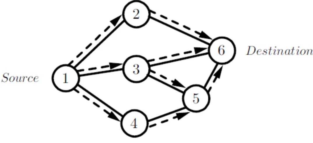
broadcasted one hop away. When a source node wishes to communicate with another node and it lacks a valid route to that node, a path discovery process is initiated. In the path discovery process the source node broadcasts a route request (RREQ) packet to its neighbors. The neighbors reply with a route reply (RREP) packet if they have a valid route to the destination node oth-erwise they broadcasts a RREQ packet to their neighbors. Figure 2.2 shows how a RREQ packet is propagated trough the network from the source node toward the destination node. In this figure it is assumed that no intermediate nodes know the route from source to destination.

Figure 2.2: Propagation of a RREQ packet through the network.

Every time a new RREQ packet is broadcasted from the source, a se-quence number called broadcast id is incremented. If a node receives a RREQ packet with a sequence number that is less or equal to a previous received RREQ packet, it drops the packet. A RREQ packet has two other sequence numbers in addition to broadcast id; source sequence number and destina-tion sequence number. The source sequence number indicates how fresh the

route information is for the reverse path to the source. The destination num-ber which specifies how fresh a route to the destination is. When a RREQ packet is broadcasted through the network, a reverse path is built from all nodes back to the source. When a intermediate node has a valid route en-try toward the destination, it compares the destination sequence number in the RREQ packet with the destination sequence number available in its own routing entry. If the destination sequence number in the RREQ packet is greater than the destination sequence number in the routing entry then it must not respond with a RREP. This is done to avoid outdated information to be transmitted. On the other hand the intermediate node should rebroad-cast the RREQ packet. When the routing entry in the intermediate node has a greater or equal destination sequence number with respect to the one in the RREQ packet, it unicasts a RREP packet back to the node from which it received the RREQ packet. Once a route toward the destination have been

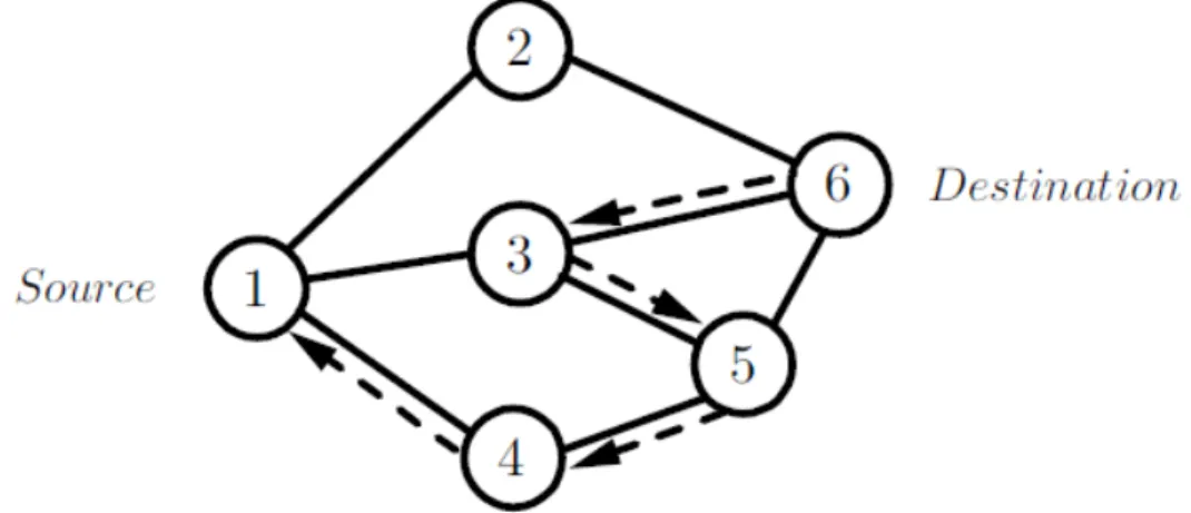
Figure 2.3: Propagation of a RREP packet.

destination node or from a intermediate node will then be unicasted along the reverse path and all intermediate nodes updates their routing entries to include the node from which the RREP came. Figure 2.3 shows the route for the RREP packet. This route is in fact the reverse path established from the propagation of the RREQ packet.

2.4

DSR

The Dynamic Source Routing protocol was proposed by Maltz et. al in [31]. DSR is a reactive protocol which uses source routing [43]. When a node wishes to send a packet to another node it includes a source route in the packets header. This source route is a sequence of nodes addresses which the packets must traverse in order to reach the destination. The packet is sent to the first hop. If a node receives a packet and it is not the final destination, it just forwards the packet to the next hop in the source route. Each node maintains discovered routes in a cache. Whenever a node wants to send a packet, it consults its route cache for a route. If a source route to the destination exists, then the node can proceed as described above. However if no source route toward the destination can be found in the route cache, a route discovery process is initiated.

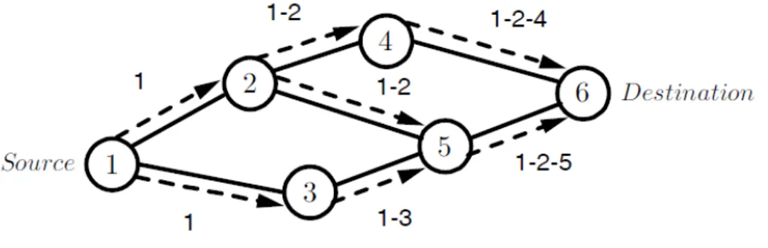
In the route discovery process the source node broadcasts a route request packet. Every route request contains source address, destination address and a unique identification number. If a intermediate node lacks a route to the destination it adds its address to the route record of the packet and forwards it on its outgoing links. Figure 2.4 shows how a route request is propagated

Figure 2.4: Propagation of a route request and building of the source record. through the network. Once a route request has reached the destination or an

Figure 2.5: Propagation of route reply by using the reversed source record.

intermediate node which knows a route to the destination, a route reply is generated. When the destination node generates the route reply it adds the information from the route record into the route reply. If an intermediate node generates the route reply it appends the route record with the route found in the route cache and adds it to the route reply. If symmetric links are supported the route reply uses the reversed route found in the route record. Otherwise the route reply packet can be piggybacked on a route request packet. Figure 2.5 shows the propagation of a route reply using the reversed source record. Once a route has been establish it needs maintenance

and for this purpose route error packets are generated at link failures. All nodes who receive a error packet removes the failed hop from the route cache and truncate all routes, containing this hop, to the previous hop. One of the advantages DSR has is that it can use promiscuous listening to learn about routes without transmitting any control packets. It works as follows; if a node a receives a packet that is targeted for a different node it can check whether a shorter route exists by sending through the node itself. In such a case a route reply is sent to the source identified in the source route. Route discovery in DSR is similar to AODV but there are some differences. DSR packets need to carry a complete source record while AODV packets only need to contain destination address which will lead to a lower overhead. The downside with AODV is that it requires symmetric links instead of DSR.

2.5

Topology Maintenance in Wireless

Net-works

Network topology is generally managed through hosts space clustering. When base stations are not present some of the hosts are elected as special nodes to guarantee intra and inter clusters communication. In the presence of base stations, hosts are clustered and each cluster is equipped with a base sta-tion. Inter cluster communication is ensured through a backbone. In these models hosts clustering is performed in a distributed fashion since a central-ized algorithm would cause heavy overhead in network knowledge collection. Closest-base clustering strategy may not guarantee good network reliability.

For this reason, throughput functions trying to balance base station closeness and load are used. Topology management and routing in wireless networks mostly relies on clustering algorithms. Some clustering algorithms have been developed for ”pure” ad-hoc networks in which hosts can communicate with or without the presence of base stations.

Gerla et al. in [23] present a radio network architecture which uses a revisited lowest-ID algorithm [17]. Each node has a distinct ID and it pe-riodically broadcasts the list of nodes that it can hear (including itself). A node which can hear only nodes with ID higher than its own ID is a clus-terhead. The remaining nodes choose their clusterhead to be the node of lowest-ID among those they can hear. Clusterheads are not linked through a backbone. Inter-cluster routing is realized by gateways: nodes that can hear two or more clusterheads. Moreover, in order to make the network more reliable, the notion of distributed gateway is introduced. In [33], Kwon and Gerla extended the Lowest-ID based algorithm by power and interference control mechanisms. Each clusterhead adjusts the signal level in order to minimally guarantee correct intracluster communication.

Lin and Gerla in [34] propose a two-hop distributed clustering algorithm without clusterheads. Nodes are divided into small groups with two-hop intra-cluster communication as in [23]. Communications across clusters are guaranteed through repeaters which are nodes that can communicate with nodes of different clusters. They also introduced a bandwidth routing algo-rithm based on Destination Sequenced Distance Vector (DSDV) for multi-media applications. The goal is to find the shortest path such that the free bandwidth is above the minimum requirement. When links fail because of

mobility, then the routing algorithm is capable of finding new routes main-taining secondary paths.

Basagni in [5] presents two distributed clustering algorithms for ad-hoc networks. The first (Distributed Adaptive Clustering) is suitable for low mobility ad-hoc networks. Nodes grouping and clusterheads selection fol-low a weight-based criterion. The second algorithm (Distributed Mobility-Adaptive Clustering) is designed for high-mobility networks. Each node dy-namically decides its role (clusterhead, ordinary) on the basis of the local network topology.

Gerla et al. in [22] propose a passive clustering in which a clusterhead is the node that sends a data packet first. Nodes in the radio coverage of this clusterhead are aggregated to it.

McDonald and Znati [36] propose an event-driven distributed clustering algorithm to aggregate nodes according to node mobility in order to balance the tradeoff between proactive and demand-based routing. A path connecting each pair of nodes in a cluster exists with a time-depending probability.

Alzoubi [3] presents two distributed heuristics to construct an approxi-mate minimum connected dominating set used as a virtual backbone for rout-ing in a wireless network. The topology is modeled as a unit disk graph [12]. This is a geometric graph in which there is an edge between two nodes if and only if their distance (number of hops) is at most one.

Banerjee and Khuller in [4] propose an algorithm to organize wireless nodes in clusters with a set of properties. Even though the program has been explicitly written for wireless sensors networks, it can be easily adapted to mobile networks in which nodes are quasi-static. The algorithm creates

different layers in which it builds a set of clusters.

In [49] Kaixin and Gerla observe that in large ad-hoc networks a flat topology is a bottleneck for the performance. A two level hierarchical ad-hoc network with two independent routing protocols is introduced. A clustering technique based on random timers is used to partition hosts into small groups. Any node not belonging to a cluster starts to build a new cluster by sending a packet to claim itself as a clusterhead. All neighbors become members of the new cluster. The random timer is used to reduce conflicts. A modified AODV protocol has been used in order to keep hierarchy into account.

Foudriat et al. in [21] present a hierarchical network in which the lowest level is the cluster served by a mobile base station. At the top of the hierar-chy there is a leader base station that is dynamically elected by the others. The leader base station periodically broadcasts the network topology. It is assumed that at least one base station has sufficient transmitting power to be heard by all clusters.

Lu et al. [35], propose a multilevel hierarchical mobile wireless network with movable base stations. The network is modeled as a tree in which mobile nodes are organized in hierarchical groups and each of them has a representative base station.

In [24] Gerla et al. present a hierarchical model similar to passive clus-tering for high speed wireless mobile backbone networks. The network is designed for battlefield operations in which unmanned flying nodes are orga-nized in clusters. At low altitude clusters perform combat missions, whereas at mid altitude nodes execute surveillance and reconnaissance operations. The highest altitude nodes provide the connectivity. In order to perform

routing the LANMAR protocol is adapted to deal with movable base sta-tions.

In [45], Srinivas et al. focus on minimizing, placing and mobilizing the base stations in a mobile backbone network under two constraints: each host is covered by a base station and the backbone is connected. Base stations placement has been formulated in terms of Connected Disk Cover problem.

In [44], Srinivas and Modiano address the joint problem of placing a fixed number of mobile base stations in the plane assigning each host exactly one base station. The assignment is modeled by maximizing the minimum or the total throughput.

2.6

Mobility Models

The performances of a wireless network protocol are strictly related to the movement of its actors [10]. Due to the lack of real data, several mobility models have been designed to capture different type of realistic actor behav-iors. In [10], authors give a survey on mobility models together with their impact on the performances of protocols.

One of the most simple and widely used mobility model is the Random Walk [16] (RWM). In RWM each host carries a speed and a direction. This information is randomly updated after a random interval of time. Bound-aries are present in the simulation. When hosts reach the boundary they continue to move in the opposite direction with respect to the incoming an-gle. The model is unrealistic since it produces sharp turns, sudden stops and it tightly depends on the time parameter. The Random Waypoint Mobility

Model (RWPM) [30] is a slight modification of the RWM. Each mobile node randomly chooses a speed and a destination in the simulation area. When the node reaches the destination point, it pauses for a while (randomly cho-sen) and then restarts. Notice that, RWPM is RWM when the sleep time is set to zero. Sharp turns and sudden stops are avoided in [7], where directions and speed values are computed according to RWPM. This allows a smoother nodes movement. In [10] the elimination of sharp turns and sudden stops is managed through a mixed Gauss-Markov model.

In [26, 37, 26] hosts are grouped together in order to reflect relationship among them and they move according to the trajectory of their group. In the Reference Point Group mobility model [26] (RPGM) each group has a logical center, called Reference Point (RP) which defines the entire group motion behavior. In each group, global speed and direction are assigned to the RP. In addition local speed and direction are assigned to each host. In order to move a host (assigned to a RP), first the RP moves according to a motion vector, then a new host position is generated by adding a random motion vector to the new RP.

Authors in [28, 29] deal with obstacles. They observe that in the real world, movement patterns do not follow a random model, they tend to select a specific destination and follow a defined path to reach the destination, avoiding obstacles to the movement. Movement paths are realized through Voronoi [41] diagram of obstacle vertices. Hosts are placed across the paths. They move towards a destination using shortest paths. Intuitively, pathways tends to lie among adjacent obstacles and Voronoi diagrams of obstacles capture exactly this concept. Performance of the AODV [40] protocol is

highly influenced by the associated mobility model. Indeed, using the above realistic protocol negatively affects efficiency with respect to the unrealistic random models.

In [32] Kim et al. define a mobility model based on real traces. Synthetic pathways generated by the model are compared with the real one showing a median relative error of 17%. Although the mobility model is more re-alistic than others, it is based on a single real trace data (the Dartmouth college). Furthermore its usage relies on the availability of real traces which are generally difficult to be known.

Chapter 3

Space Coverage Optimization

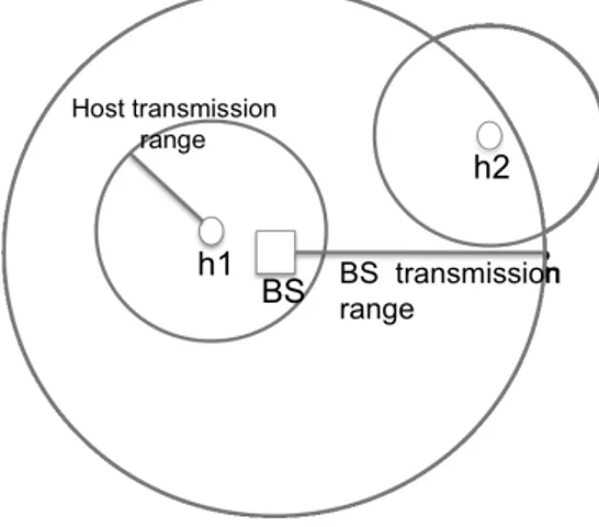
One of the main goals of a wireless network with movable base stations is to minimize uncovered areas. A host is covered by a base station if a bidirec-tional transmission link can be established. Consequently, each covered host has a base station within its transmission range (see Figure 3.1). Clustering

Figure 3.1: Transmission ranges: host h1 is covered, h2, although is in the transmission range of BS it will not be able to communicate since BS is not in its transmission range.

techniques allow to optimize space coverage by locating base stations in the clusters’ centroids. Hosts are periodically clustered and each base station moves to an assigned centroid of a cluster. Two scenarios are possible: (i) if a base station knows all the hosts and the base stations positions, clustering can be performed by a centralized algorithm; (ii) if each base station has only a local knowledge, a distributed clustering is needed. If obstacles are present, they obstruct base stations and hosts movements and may also inter-fere transmission. In this situation, base stations repositioning is performed by a bipartite matching algorithm properly adapted to deal with obstacles as shown below. Finally, good performances of clustering and repositioning algorithms should be guaranteed during the evolution of the network. In this thesis we use an efficient hierarchical clustering algorithm Antipole Tree Clustering properly adapted to this scenario. In section 3.1, we sketch the sequential version of Antipole Tree Clustering in starred networks [20]. Next, in section 3.2, we propose a distributed version of the Antipole Tree Cluster-ing and its application to MBWN. In section 3.3 we introduce a fast motion planning model to reposition base stations in the presence of obstacles.

3.1

The Antipole Clustering in Mobile

Wire-less Network with Starred Backbone

repositioned according to a fast closest match algorithm which minimizes both total and maximum distance [20].

Notice that if the number of base stations is different from the number of clusters the matching algorithm can be still applied by merging clusters or switching off the unused base stations.

The Antipole Tree Clustering algorithm (see Fig.3.2) is based on the ob-servation that distant elements lie in different clusters. The algorithm finds a pair of distant element A, B (Pseudo-Diameter) in linear time with an

ap-proximation ratio of 1/√2 with respect to the exact Diameter. It partition

elements according to their proximity to one of the endpoints A, B. This top-down recursive splitting procedure will produce a binary tree whose leaves are the final clusters. Assume that a cluster radius σ, which guarantees good

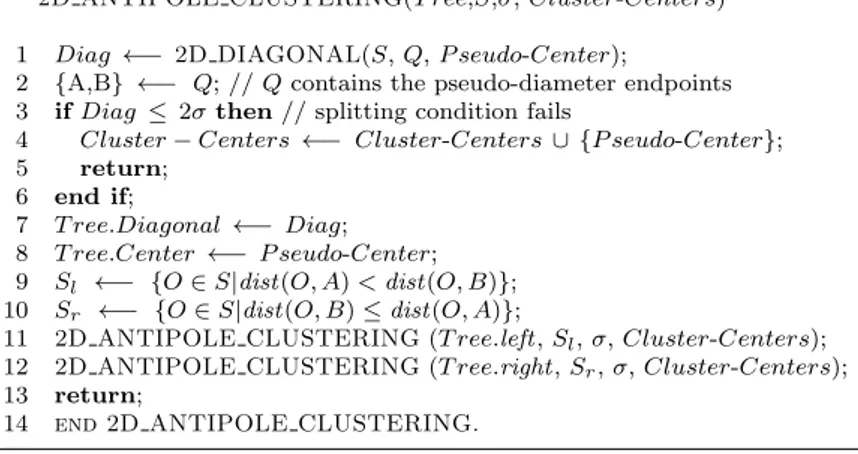
2D ANTIPOLE CLUSTERING(T ree,S,σ, Cluster-Centers)

1 Diag ←− 2D DIAGONAL(S, Q, P seudo-Center);

2 {A,B} ←− Q; // Q contains the pseudo-diameter endpoints

3 if Diag ≤ 2σ then // splitting condition fails

4 Cluster− Centers ←− Cluster-Centers ∪ {P seudo-Center};

5 return;

6 end if;

7 T ree.Diagonal ←− Diag;

8 T ree.Center ←− P seudo-Center;

9 Sl ←− {O ∈ S|dist(O, A) < dist(O, B)};

10 Sr ←− {O ∈ S|dist(O, B) ≤ dist(O, A)};

11 2D ANTIPOLE CLUSTERING (T ree.left , Sl, σ, Cluster-Centers);

12 2D ANTIPOLE CLUSTERING (T ree.right , Sr, σ, Cluster-Centers);

13 return;

14 end 2D ANTIPOLE CLUSTERING.

Figure 3.2: Euclidean 2-dimensional Antipole Algorithm.

communication between each host and its base station, is given. The Antipole clustering of bounded radius σ [11], starting from a given finite set of points

S, checks if the Pseudo-Diameter is greater than 2× σ (splitting condition).

is a cluster. Otherwise, the set is partitioned by assigning each point of the

splitting subset to the closest endpoint of the Pseudo-Diameter {A, B}. In

the plane this procedure can be efficiently performed in the following way. At

each step, let T be the splitting subset to be processed, and let (PXm, PXM)

and (PYm, PYM) be the four points of T having minimum and maximum

Carte-sian coordinates. Notice that, these four points belong to the convex hull of T . The diameter of these four points is the Pseudo-Diameter of T . Moreover the

splitting condition for T is√(PXm.x− PXM.x)

2_{+ (PY}

m.y− PYM.y)

2 ≥ 2×σ,

where P.x and P.y are the coordinates of the point P . If the splitting con-dition is satisfied then the diagonal of the rectangle is greater or equal than 2× σ. Since the Pseudo-Diameter is at least Diagonal/√2, this yields that

P seudo−Diameter

2×σ ≥ 1

√

2 (see Fig.3.3 for the pseudo code of the algorithm). This

proves that the approximation ratio is 1/√2. On the other hand, if the

split-ting condition is not satisfied, then the partition is not performed and the subset is one of the clusters. The middle point of the rectangle diagonal is the Pseudo-Center of the cluster (see Fig. 3.2 for the pseudocode).

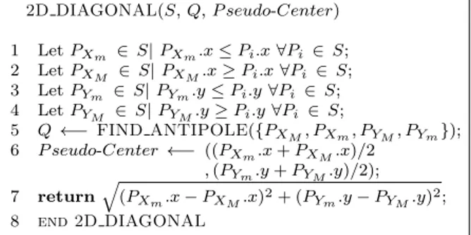
2D DIAGONAL(S, Q, P seudo-Center) 1 Let PXm ∈ S| PXm.x≤ Pi.x∀Pi ∈ S; 2 Let PXM ∈ S| PXM.x≥ Pi.x∀Pi ∈ S; 3 Let PYm ∈ S| PYm.y≤ Pi.y∀Pi ∈ S; 4 Let PYM ∈ S| PYM.y≥ Pi.y∀Pi ∈ S; 5 Q←− FIND ANTIPOLE({PXM, PXm, PYM, PYm}); 6 P seudo-Center←− ((PXm.x + PXM.x)/2 , (PYm.y + PYM.y)/2); 7 return√(PXm.x− PXM.x)2+ (PYm.y− PYM.y)2; 8 end 2D DIAGONAL

Figure 3.3: The algorithm to find the diagonal, the Pseudo-Diameter and the Pseudo-Center.

Antipole Clustering. Here the splits occur also when the cardinality of the subset is larger than the size threshold k. This helps to satisfy throughput constraints (the condition to check the size of the cluster can be inserted between lines 3 and 4 in the pseudocode of Fig. 3.2).

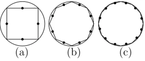
In order to obtain an exponentially arbitrary low approximation ratio δ of the real diameter a bisecting algorithm is provided (see the pseudocode in Fig. 3.4). Performing a π/4 rotation of the Cartesian coordinates implies a bisection of the axes. Compute then, the maximum and minimum coordinate points for such two new axes, this yields a set of 8 points. Let (A, B) be the

diameter of this set. Plainly, dist (A, B)/ cosπ₈ > Diameter ( Fig. 3.5 (b)).

By iterating this bisection process d times we have dist (A, B)/ cos₂d+2π >

Diameter. Therefore, the approximation ratio is

δ = |Diameter − P seudo Diameter|

Diameter ≤  1 − cos π 2d+2   . This yields the following Lemma:

Lemma 3.1.1. Let S be a set of points in the plane and let 0 < δ ≤

1 − 1/√_{2. Then a call to APPROX DIAGONAL(S, δ) returns an}

An-tipole pair (A, B) (P seudo Diameter) which approximates the diameter with

APPROX DIAGONAL(S, δ)

1 Let BBox ={PXm, PXM, PYm, PYM} be the minimum bounding box of S;

2 V ← {{S}};

3 for i = 1 tod_{4×arccos(1−δ)}π − 1e do

4 V0 = ROTATE SET(V,₂i+1π

) ; 5 Let BBox π

2i+1 ={PXm, PXM, PYm, PYM}

be the minimum bounding box of the rotated sets in V0;

6 V = Set catalog of V0;

7 BBox = BBox∪ BBoxi;

8 end for

9 return FIND ANTIPOLE(BBox);

Figure 3.4: Algorithm for the Pseudo-Diameter Computation.

(a) (b) (c)

Figure 3.5: The worst cases in the first three iterations of algorithm in Fig.3.4.

3.2

Distributed Antipole Clustering and Base

Stations Repositioning in Absence of

Ob-stacles

Following [19], let n be the number of base stations and m be the cardinality of a set S of hosts. The algorithm partitions the hosts in disjoint subsets. Base stations occupy the centers of such sets. Suppose that the backbone has a specific interconnection topology such as a Euclidean Minimum Spanning Tree (EMST). Stations communicate through messages and each message is correctly transmitted to a unique successor which is its father in the EMST. There is one designated final base station f called root (not necessarily always the same) aggregating the results of all local computations.

Initially, the root f contains all the base stations coordinates, cold

i , before

the motion. After the motion, reclustering could be necessary. In such a case, the following steps of Distributed Antipole Clustering (DAC) procedure

produces a set of new clusters, Cnew

i , piecewise distributed among the base

stations and whose centers, cnew

i , are all stored in the root f .

1. Grouping: Each base station j sends an Hello message to hosts in order to build the group of nodes that it can hear.

2. Local enclosing box computation: Each base station j in the leaf

in the EMST, computes the enclosing box {P_Xj

m, P j XM, P j Ym, P j YM} of

its local set of hosts Sj _{and passes such a bounding box to its father}

through a message of fixed length (see Figure 3.6 (a)).

3. Global enclosing box computation: Each internal node in the EMST receives enclosing boxes from its children and merges them with its local enclosing box. This merging results in the enclosing box of the enclosing boxes. This new enclosing box will be recursively propa-gated through the tree by using a fixed length message. At the end of this process the root station f will store the global enclosing box

{PXm, PXM, PYm, PYM}.

4. New cluster and center computation: If the semi-diagonal of the global enclosing is smaller than the cluster radius threshold (commu-nication radius) the root f sends a termination message to all stations (see Figure 3.6 (b)). Then, a base station will occupy the new center,

cnew

5. Cluster splitting phase: If the previous step does not apply, the root

f broadcasts the farthest pair (global Antipole (A, B)) of the global

enclosing box (see Figure 3.6 (b)). Each station, after receiving the global Antipole (A, B), splits its local data according to the distance from A and B. The algorithm proceeds recursively until splittings no longer occur.

6. Termination: When the splitting procedure is completed, each base

station, j, contains the local portion, C_inew,j, of hosts for every cluster,

Cnew

i . The root f contains all the cluster centers cnewi .

7. Base stations repositioning in absence of obstacles and

back-bone reconfiguration: The root f , knowing the old, cold_i , and the new

centers, cnew

j , computes, through a bipartite matching algorithm

(Clos-est Match [20] which tries to minimize the total distance covered by the base stations motion), the new position of each base station. Next, it calculates the new backbone EMST and the new root node. Such a node is the center of the EMST balancing the tree. Such a choice allows to minimize the number of hops needed to reach every base sta-tion during the clustering phase. Finally, the root f communicates to each station its new destination and the base stations reposition, accordingly (see Figure 3.6 (b)).

Concerning the last paragraph listed above, the computation of the new root node takes into account what follows [8]:

Lemma 3.2.1. For any tree, the center of a tree consists of at most two

(a) (b)

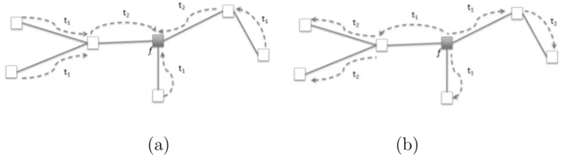
Figure 3.6: (a) Propagation of Local Enclosing Box Messages (Step 2 of the

distributed Antipole Clustering algorithm). At time t1 each leaf computes

the local enclosing box and sends it to its father. Each internal node in

the EMST merges the received enclosing boxes with its own. At time t2,

the internal nodes propagate the new enclosing boxes to the root station f which will compute and store the global enclosing box. (b) Propagation of messages from the root station f to the base stations through the EMST (Steps 4, 5, 7 of the distributed Antipole Clustering algorithm algorithm).

The proof of the lemma is trivial and gives a way to compute the center of the tree just by recursively deleting the leaves.

The above lemma implies that, in principle, each base station can be designated as a root in the Euclidean spanning tree. The root does not need extra energy because the additional effort required is only the computation of new base stations destinations. This allows to randomly change the root base station according to the current spanning tree.

The DAC algorithm is periodically executed by the base stations upon a request from the root. For each time interval ∆t (20 seconds in our

sim-ulation), the root f collects the percentage of covered hosts ht obtained

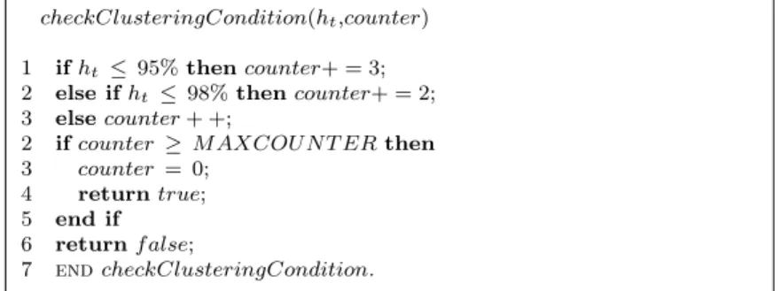
from the sum of covered hosts given by each base station. Then, the root performs a counter based procedure (see Figure 3.7) to decide whether a clus-tering is needed. A global variable counter, initially set to zero, is increased

M AXCOU N T ER (3 in our simulation), a new clustering starts and the counter is reset. From figure 3.7 we can see that, if the percentage of covered

checkClusteringCondition(ht,counter)

1 if ht ≤ 95% then counter+ = 3;

2 else if ht ≤ 98% then counter+ = 2;

3 else counter + +;

2 if counter ≥ MAXCOUNT ER then

3 counter = 0;

4 return true;

5 end if

6 return f alse;

7 end checkClusteringCondition.

Figure 3.7: Clustering Condition Check. At each round a counter based check is performed. If the procedure returns true, a new clustering starts.

hosts falls below 95% then a new clustering will start. If the percentage of covered hosts falls below 98% a new clustering, at next round in the worst case will start (but it can start also instantly if counter reaches or exceeds

M AXCOU N T ER). Otherwise, counter will be increased by one. This

en-sure that, in the best case (i.e. in each round the percentage of covered hosts is above 98%), the clustering procedure will start anyway after three rounds (60 seconds in our simulation) allowing a better organization of the topology. Since the Antipole Clustering does not guarantee that the number of clusters’ centroids is equal to the number of base stations (i.e. the number of destinations may differ from the number of base stations), the root f proceeds accordingly:

• If the number of centroids is less than the number of base stations, some

of such base stations (the furthest from the centroids) stay idle but still used for communications. This is achieved without any additional cost by the matching algorithm which will match only the correct number

of base stations leaving unmatched the exceeding ones.

• When the number of clusters exceed the number of base stations,

clus-ters are merged hierarchically (i.e. by using neighbor-join [6]) until the right number of clusters is reached.

3.3

Clustering and Base Stations

Reposition-ing in Presence of Obstacles

In a real situation base stations move in a relatively open space in presence of obstacles (i.e. hills, rivers, buildings, urban roads etc). Without loss of generality, in our proposed algorithm, we approximate obstacles by their minimum bounding rectangle containing it and whose sides are parallel to the coordinate axes. With the presence of obstacles we extend the protocol described in Section 3.2 to capture the following scenarios.

Obstacles may obstruct the signal propagation. Nodes that are

obstructed by obstacles may still be able to communicate, but the received signal has lower power level. Therefore, we introduce a signal attenuation

factor, Atranging from 0 to 1 (At=0 means that obstacles do not influence the

transmission, At=1 indicates that obstacles completely obstruct the signal

propagation).

Cluster centers may fall within an obstacle. In order to ensure that

target positions are always placed outside obstacles, we modified the step 4

in Section 3.2 as follows. If the center of the global enclosing box cnew_i falls

of the obstacle. Then, if the furthest vertex of the cluster enclosing box is greater than the cluster radius threshold (communication radius), the root f splits the cluster (go to step 5 in the preceding Section). Otherwise it sends the termination message with the new cluster center.

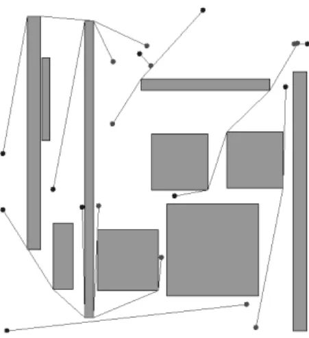
Obstacles may obstruct the paths of base stations. In this case,

we choose to minimize the parallel motion time needed to complete the repo-sitioning (i.e. we minimize the maximum distance). For this purpose we adpated the Bottleneck Matching algorithm [1] on Visibility Graphs [9, 47]. On the other hand, the Minimum Weight Bipartite Matching algorithm [2] can be used to minimize the total distance covered by the base stations. More precisely, we perform base station repositioning in the following way. Let G(V, E) be the visibility graph [47] constructed on the set O of obstacles vertices, let cold={cold₁ , cold₂ ,· · · , cold_n } be the current base stations positions,

and let cnew ={cnew₁ , cnew₂ , · · · , cnew_n } be the base stations destinations.

Edges are weighted, w, with the Euclidean distance. Distances between pair of nodes are given by the Dijkstra algorithm [13]. A matching M , called

bottleneck match, is a collection of n paths π1, π2,· · · , πnconnecting sources,

cold_{, to destinations, c}new_{, in a one-to-one fashion. A bottleneck match}

mini-mizes the parallel time function: P TM(cold, cnew) = max1≤i ≤n

∑

e∈ πiw(e)

1_.

In order to simplify presentation, we assume the absence of collisions among base stations during the motion (see [9] for collisions avoidance). In what follows we give a sketch of the steps of the bottleneck matching.

1. Initialization: Initialize D to be an ordered set of all shortest path

1_{This problem with the condition stating that two paths cannot collide is}

NP-complete [15]. By relaxing such a condition (disjointness of the paths) the problem becomes polynomial.

distances among pairs of sources and destinations (cold

i , cnewj ).

2. Iteration: Let m be the median of D, search for a match M such that

P TM(cold, cnew) ≤ m.

• Match found: If a match M of cardinality n exists, then try to

find a match recursively on the first half D.

• Match not found: try to find a match recursively on the second

half of D.

3. Termination: The search stops when current D is empty. The last successful match M represents the output of the algorithm.

The key step of the bottleneck matching algorithm is the construction of the partial matching during the above binary search strategy. Starting from a

match M , construct incrementally a match of cardinality|M|+1. The notions

of alternating and augmenting walks are introduced. A current match M in

the visibility graph G(V, E) is a set of paths starting from a node of cold and

ending in a node on cnew_{. We label those nodes matched and the remaining}

ones exposed. Notice that internal nodes of a path in M , if any, can be only vertexes of obstacles.

A path π = (v1 v2 v3 . . . v2t) is called an alternating walk

if:

1. v1 is an exposed vertex of cold and v2t is in cnew;

2. all the paths (v2i v2i+1) ∈ M, with i = 1, · · · , t − 1, and (v2i−1

v2i), with i = 2, · · · , t, are paths in G which are not in M and their

Figure 3.8: An example of Bottleneck matching in the presence of obstacles. Each obstacle is approximates by its minimum bounding box.

An alternating walk is called an augmenting walk if v2t is exposed. If π is an

augmenting path then M0 = (M\{∪i=1,...t−1(v2i v2i+1)}) ∪ {∪i=2,...t(v2i−1

v2i)} (obtained by removing from M the paths of π belonging to it and adding

the remaining paths of π) is a match and |M0| = 1 + |M|.

Complexity Analysis. The complexity of the proposed algorithm is

higher than the corresponding Euclidean version since basic computational geometry data structures are not available on graphs. Given h obstacles and

n base stations, each obstacle bounding rectangular box has 4 vertices, and

for each base station there is a starting and ending position, than the total number of nodes in the visibility graph will be 2n + 4h. If the visibility graph has k edges, then by extending the arguments of [1] the complexity of the

Chapter 4

Throughput Optimization and

Network Maintenance

Communication among hosts in our model is guaranteed by a two level hi-erarchy architecture (see Figure 4.1). In the first level, a host who wants to communicate sends a message to the joint base station. In the second level, by using the standard AODV, base stations identify the route to reach the destination host. The communication is guided by the AODV proto-col. Therefore, the backbone used for communication differs from the one adopted during the clustering (i.e. the EMST).

Since hosts frequently move, to maintain up to date the network and to optimize the base stations load, hosts are periodically assigned according to a probabilistic throughput function. The throughput combines the quality of the signal (influenced by the presence of obstacles and in general inversely proportional to the distance host - base station) and the potential load of the base stations due to the number of hosts in their neighborhood. Each host

Figure 4.1: The two level hierarchy architecture

computes such a function yielding a score that identifies the best base station to join with. Since we use a single communication channel (802.11x protocol) the throughput achieved by a host transmitting to its assigned base station is influenced by the totality of the hosts in the same neighborhood and not only by those joint with the base station [48]. For this reason, models based on channels separation [45, 44] cannot be applied.

More precisely, hosts assignment is achieved in the following way.

Sim-ilarly to the AODV, each host hj periodically (i.e. every 3 seconds in our

simulation) receives an HELLO message with a certain quality (inversely proportional to the distance) from the base stations which it can hear. Each HELLO message, sent by the base station, BSi, contains ni, the number of

hosts reachable by BSi (i.e. number of hosts assigned to such a base station

plus the hosts in its neighborhood which answered to the previous HELLO

message). Suppose that the host hj can hear k base stations, each of them

hj will join the i-th base station is defined as follows: T P (pij, ni) = pij (ni+1)α ∑k l=1 plj (nl+1)α

It is easy to see that fixed a base station, T P () is directly proportional to the power of the HELLO message sent and it is inversely proportional to the number of hosts in the base station neighborhood. The denominator is used to normalize T P () in the [0, 1] interval.

In the experimental section we show that T P () allows to increase the percentage of delivered messages with respect to an assignment based only on distances.

Although the host assignment based on the T P () function works well in practice, it is a heuristic assignment and it can not guarantee the best allocation.

Finally, notice that, the above network maintenance is also performed during base station repositioning (see Figure 4.2). This ensures hosts com-munications and avoids network stalls.

Figure 4.2: Network infrastructure temporal maintenance. After the first 20 seconds a clustering is needed and thus performed. On the contrary, the second check condition results false and the clustering does not start. In order to ensure network maintenance, base stations send HELLO messages also during clustering and repositioning.

Chapter 5

Introduction to NS2

5.1

NS2 Network Simulator

Network Simulator (Version 2), widely known as NS2, is a powerful event-driven simulation tool that has been widely used in studying the dynamic nature of communication networks. Through NS2, wired and wireless net-works functions and protocols (e.g., routing algorithms, TCP, UDP) can be simulated and analyzed. In general, NS2 provides users with a way of specifying such network protocols and simulating their corresponding behav-iors. Due to its modular nature, NS2 has gained constant popularity in the networking research community. Thanks to substantial contributions from several research group, extensions and revisions have marked the growing maturity of the tool. NS2 is an evolution of Network Simulator 1 devel-oped through a joint project between University of California and Cornell

University. Since 1995 the Defense Advanced Research Projects Agency (DARPA) supported development of NS through the Virtual InterNetwork Testbed (VINT) project. Currently the National Science Foundation (NSF) has joined the development project. Last but not the least, there is a wide community of researchers and developers who constantly work on NS2. Fig-ure 5.1 shows the basic architectFig-ure of NS2. NS2 provides users with an executable command ns which takes as input the name of a Tcl simulation scripting file. In most cases, a simulation trace file is created, and is used to plot graphs and/or to create animations. NS2 consists of two key

lan-Figure 5.1: Basic architecture of NS.

guages: C++ and Object-oriented Tool Command Language (OTcl). While the C++ defines the internal mechanism (i.e., a back-end) of the simulation objects, the OTcl sets up simulation by assembling and configuring the ob-jects as well as scheduling discrete events (i.e., a front-end). The C++ and the OTcl are linked together using TclCL [18]. Mapped to a C++ object. The variables in the OTcl domains are sometimes referred as handles.

Con-ceptually, a handle (e.g., n as a Node handle) is just a string (e.g., o10) in the OTcl domain, and does not contain any functionality. Instead, the func-tionality (e.g., receiving a packet) is defined in the mapped C++ object (e.g., of class Connector). In the OTcl domain, a handle acts as a front-end which interacts with users and other OTcl objects. It may defines its own pro-cedures and variables to facilitate the interaction. The member propro-cedures and variables in the OTcl domain are called instance procedures (instprocs) and instance variables (instvars), respectively. NS2 provides a large number of built-in C++ objects. It is advisable to use these C++ objects to set up a simulation using a Tcl simulation script. However, users could need to develop their own C++ objects, and use a OTcl configuration interface to put together these objects.

After simulation, NS2 outputs either text-based or animation-based sim-ulation results. To inspect these results graphically and interactively, tools such as NAM (Network AniMator) can be used. NAM is a Tcl/TK based animation tool for viewing network simulation traces and real world packet traces. It supports topology layout, packet level animation, and various data inspection tools. NAM however is not able to show items such as obstacles. To work around this limitation we used fake wired networks (see figure 5.2), irrelevant to the simulations.

To analyze a particular behavior of the network, we can extract subsets of text-based data and transform them into a more conceivable presentation. Simulation data is acquired from trace-files which NS2 generates. Trace-files can either filtered at runtime by using a script or can be written directly to disk. Both methods present drawbacks. Filtering at runtime could discard

Figure 5.2: NAM example.

relevant data, writing to disk may take too much time and trace-files from simulations could need many Gigabytes of space. Our model of simulation re-quires a OTcl script for network configuration, a mobility pattern describing nodes movement, a traffic pattern describing data traffic and a file describing coordinates obstacles.

5.2

Layers into NS2

A computer network is a complex system. To facilitate design and flexi-ble implementation of such a system, the concept of layering is introduced. Using a layered structure, the functionalities of a computer network can be organized as a stack of layers. There is a peer-to-peer relationship (or virtual link) between the corresponding layers in two communicating nodes. How-ever, actual data flow occurs in a vertical fashion from the highest layer to the lowest layer in a node, and then through the physical link to reach the lowest layer at the other node, and then following upwards to reach the high-est layer in the stack. Each layer represents a well-defined and specific part of the system and provides certain services to the above layer. Accessible (by the upper layers) through so-called interfaces, these services usually define

what should be done in terms of network operations or primitives, but does

not specifically define how such things are implemented. The details of how a service is implemented is defined in a so-called protocol. For example, a source node transmitter can use at the physical layer a specific protocol (e.g., a data encoding scheme) to transmit data to a receiver, which should be able to decode the received information based on the protocol rules. The beauty of this layering concept is the layer independency. That is, a change in a protocol of a certain layer does not affect the rest of the system as long as the interfaces remain unchanged. Here, we highlight the words services, protocol, and interface to emphasize that it is the interaction among these components that makes up the layering concept. As shown in figure 5.3 NS2 works with layers, where each layer is a module or a set of modules written

Figure 5.3: Layers into NS2. in C++.

5.2.1

Physical Layer

Physical layer (often termed PHY) is referring to network hardware, physical cabling or a wireless electromagnetic connection. It provides an electrical, mechanical, collision control and procedural interface to the transmission

medium. The Physical Layer defines the means of transmitting raw bits rather than logical data packets over a physical link connecting network nodes. The bit stream may be grouped into code words or symbols and converted to a physical signal that is transmitted over a hardware transmis-sion medium. The physical layer is the very simplest, defining only exactly what a bit is: in other words how to transmit a one or a zero.

The physical layer of wireless simulation in NS2 contains an important module: the Signal Propagation Model. It determines whether two nodes can communicate: by distance, signal strength and by other additional variables.

5.2.2

The Signal Propagation Model

One of the primary limitations of the performance of wireless networks is the significant attenuation and interference experienced by the radio signal as it propagates from the sending node to the receiving node. In a set-ting with obstacles, the signal may reach the receiver via non-line-ofsight propagation mechanisms, such as reflection, diffraction and scattering. This effect of multi-path propagation results in a drop in the Signal-to-Noise Ratio (SNR) of the received signal. The free-space fading models are not suitable to calculate the attenuation undergone by the signal being received. Ad-ditionally, the fluctuations of the signal levels are log-normally distributed about a mean value and the changes in the signal levels are insignificant over short periods of time, leading to a phenomena called long-term fading. In our simulations, we use either the Two-Ray Pathloss Model that accommodates the reflections of the signals off the surface of the ground, in addition to the

direct path signals from the source transceiver to the destination transceiver; or the Friis’ Free Space Equation [42] which considers only a single path of propagation. The equation is defined as follows:

P

=

2

(4πd)2

where Pr is the Power received, Pt is the power transmitted, Gt and Gr are

the antenna gain of the transmitting and receiving antennas, respectively, λ is the wavelength of the radio signal and d is the distance. The choice of

these models depends on the value of the cross-over distance, dc, where dc

is the distance such that when d = dc, the received power predicted by the

two-ray ground model is equal the one predicted by the Friis equation. Two case are possible:

• when d < dc, we use the Friis’ Equation since the power attenuated is

inversely proportional to d4;

• when d ≥ dc, we use the Two Ray Pathloss Model since the power

attenuated is inversely proportional to d2_;

In detail dc = 4πh_λthr, where ht and hr are the antenna heights of the

trans-mitter and the receiver, respectively.

The Two Ray Pathloss Model equation is defined as:

P

=

PtGtGr(hthr)2

d4

In the real world a radio signal transmitted between a pair of nodes undergoes fading, attenuation, scattering, diffraction, reflection, multipath propagation, etc. In this thesis we use empirical results to simulate these

effects. Hence, there is a possibility that two nodes that are obstructed by an object or any other natural obstacle may still be able to communicate, but the signals that are received have a lower power level. Before a simulation begins, we can specify the penetration characteristics of a obstacle. There are two extreme cases for this specification. In the case of a perfect conductor, a radio wave that is incident to the material is completely attenuated (i.e.,

Attenuation At→ ∞). On the other hand, an obstacle can be specified such

that it obstructs only movement, and not the propagation of radio signals, e.g, a river. In this case, the radio wave does not fade due to the obstacle

(i.e., At = 0 ). Hence, 0≤At≤∞. As mentioned in section 3.3, for simplicity

our At is a value between 0 and 1.

A text file, named Obstacles.txt, is used to describe the obstacles in the scenario of our simulations. For simplicity, each obstacle is represented by a rectangle (as mentioned in section 3.3), as an ordered sequence of its four

vertices whose sides are parallel to the coordinate axes, and its At value.

Starting from the standard TwoRayGround module (written in C++) of NS2 to simulate a signal propagation with Two-Ray Pathloss Model, we have developed TwoRayGroundwObs able to manage obstacles in a wireless simu-lation.

Chapter 6

Implementation and

Experimental Analysis

6.1

Implementation

In this section, we present an implementation of our model as an extension of the widely used Ad-hoc On-Demand Distance Vector [40] protocol (AODV). Such a modeling is suitable for our purposes since AODV is based on HELLO messages.

In order to simulate the presence of a base stations backbone, we adapted the AODV by introducing a two level hierarchical network organization called Two-Level-Hierarchy-AODV (TLH-AODV). As mentioned in section 5.1, NS2 is an object oriented simulator written in OTcl and C++ languages. While OTcl acts as the front-end (i.e., user interface), C++ acts as the back-end running the actual simulation. As can be seen from Fig. 6.1, class hierarchies of both languages can be either standalone or linked together

ing an OTcl/C++ interface called TclCL [18] . There are two types of classes in each domain. The first type includes classes which are linked between the C++ and OTcl domains. In the literature, these OTcl and C++ class hierar-chies are referred to as the interpreted hierarchy and the compiled hierarchy, respectively. The second type includes OTcl and C++ classes which are not linked together. These classes are neither a part of the interpreted hierarchy nor a part of compiled hierarchy.

Figure 6.1: Two language structure of NS2. Class hierarchies in both the languages may be standalone or linked together. OTcl and C++ class hi-erarchies which are linked together are called the interpreted hierarchy and the compiled hierarchy, respectively.

As discussed above, TwoRayGroundwObs implements the signal propa-gation Model in the presence of obstacles (see Sections 5.2.2 and 3.3) and TLH− AODV implements the proposed protocol (see Chapters 3 and 4). In order to generate mobility patterns, we did not use the built-in program ”setdest” of NS2 because it implements only Random Waypoint in absence of obstacles. For this reason we rewrote completely the procedure for generat-ing mobility patterns for both RWP and RPGM in the presence of obstacles. As shown in Fig. 6.2, in order to take into account the new mobility mod-els and algorithms, ad hoc parameters have been introduced in the simulation

# Define options

# Set variable Value Comment 01 set val(chan) Channel/WirelessChannel ;# Channel type

02 set val(prop) Propagation/TwoRayGroundwObs ;# radio-propagation model 03 set val(netif) Phy/WirelessPhy ;# network interface type 04 set val(mac) Mac/802 11 ;# MAC type

05 set val(ifq) Queue/DropTail/PriQueue ;# interface queue type 06 set val(ll) LL ;# link layer type 07 set val(rp) TLH AODV ;# routing protocol

08 set val(x) 900 ;# X dimension of topography 09 set val(y) 900 ;# Y dimension of topography 10 set val(stop) 1800 ;# time of simulation end 11 set val(emodel) EnergyModel ;# Energy Model

12 set val(sigma) 200 ;# SIGMA value in Antipole Clustering 13 set val(clustertime) 20 ;# Time value beetwen two clustering 14 ...

Figure 6.2: The initial portion of environment definition, written in Tcl, of a our simulation.

script.

The simulations were done using NS2 v. 2.33 under a Pentium IV 2.8GHz with 1GB RAM with Linux operating system (kernel 2.6). Table 6.1, shows the parameters used during the simulation.

Since we assume a single communication channel we do not compare our model with those presented in [44, 45] because they are based on channel separation: hosts which are close but joint with different base stations do not interfere with each other. Furthermore, in [45] the problem solved is slightly different because the number of available base stations is not bounded (in our case the number of base station is fixed a-priori). Concerning [44], the protocol is an interesting theoretical result. Indeed, it results unfeasible because of its high computational complexity. In the presented scenarios we need efficient methods to frequently reassign hosts and move base stations.

Parameter Value

Simulation area size 900m× 900m

Host-bs transmission range 150m

Bs-bs transmission range 400m

MAC 802.11 data rate 11M b/s

Wireless phy frequency 2.4GHz

Signal propagation model two ray ground (adapted to deal with

obstacles obstructing the communication)

Hosts walking speed 0.5m/s - 1.8m/s

Base stations speed 15m/s(54Km/h)

Simulation timing 1800 seconds

Number of hosts 100

Number of BS 9

CBR communication packets 2000 (between two randomly chosen hosts)

Clustering time check 20 seconds

MAXCOUNTER 3

α 0.25

Table 6.1: Simulation parameters. wireless protocols such as AODV and DSR.

In order to highlight the strengths and the weakness of our model we performed several experiments.

We ran the simulation for 100 pairs of randomly chosen connections com-paring the behavior of the protocol on two different mobility models: RWPM and RPGM. Hosts turn around obstacles when they obstruct their way and the protocol takes into account a signal attenuation factor. In the RWPM, nodes are initially randomly placed in the simulation area and move accord-ing to the model. In the RPGM, nodes are organized in groups (in our simulation we considered 10 groups) and each group moves randomly in the area. Both models take into account the obstacles randomly distributed in de simulation area. We analyzed the performances of two different versions

of our protocol: the Dynamic TLH-AODV in which bases stations move and the Static TLH-AODV in which base stations are fixed and no clustering is performed. In the latter case, base stations are placed in the simulation area in order to maximize the space covered. We performed several tests to establish the α parameter of T P () which has been set to 0.25 for all the experiments.