QUADERNI DEL DIPARTIMENTO DI ECONOMIA POLITICA E STATISTICA
Ahmad K. Naimzada Serena Sordi
On controlling chaos in a discrete tâtonnement process
On controlling chaos in a discrete
tâtonnement process
Ahmad K. Naimzada
Department of Economics, Quantitative Methods and Business Strategy, University of Milano-Bicocca
Serena Sordi
Department of Economics and Statistics, University of Siena
Abstract
The simple pure exchange model with two individuals and two goods by Day and Pianigiani (1991), extensively analyzed by Day (1994, Ch. 10) and taken up again by Mukherjy (1999), is discussed and extended with the purpose of showing that chaos in a discrete tâtonnement process of this kind can be controlled if the auctioneer uses a smooth, nonlinear formulation of the price evolution process such that the price adjustment is a sigmoid-shaped function of the excess demand, with given upper and lower limits. This formulation o¤ers some advantages over previous speci…cations. In particular, given the speed of adjustment and the excess demand function, we show that, acting on the lower and/or upper limits that constrain price dynamics, the auctioneer can (i) stabilize the dynamics, (ii) reduce the complexity of the attractor and (iii) increase the economic signi…cance of the adjustment process.
Key words: Price adjustment, tâtonnement, chaos, control JEL Classi…cation: C62, D50
Corresponding author
Email addresses: [email protected] (Ahmad K. Naimzada), [email protected] (Serena Sordi).
1 Introduction
The issue of the dynamics of the tâtonnement process has recently been subject to a renewed burst of interest. In the last thirty years or so, attention has been concentrated especially on discrete-time formulations of the process, which are capable of producing di¤erent types of complicated price adjustments to disequilibrium between supply and demand of a good. As a result, there exists by now an extensive literature on the so-called ‘chaotic tâtonnement’where it is possible, broadly speaking, to distinguish three strands of research.
In most of the early contributions (e.g., Saari 1985, 1991; Day and Pianigiani 1991; Bala and Majumdar 1992; Day 1994 and Kaizoji 1994; see also Mukherji 1999),1 the main purpose was to show that the use by an auctioneer of a tâtonnement mechanism that takes place in discrete steps makes it possible for the model to exhibit persistent chaotic behavior such that the relative price can jump erratically, and with no limits, depending on the size of the excess demand.2 When this happens, given that the price does not converge
to its equilibrium level, transactions do not take place and we can conclude that the iterative mechanism for price adjustment chosen by the auctioneer is not e¤ective. In the wake of recent developments in the theory of nonlinear dynamic systems and in particular of the idea “that it is not complexity of structure that gives rise to complex behavior but non-linearity” (Day and Pianigiani 1991, p. 38), this has been shown to hold even for the simplest possible tâtonnement process, with only two goods and two individuals. The dissatisfaction regarding the various implications of this result explains the emergence of two other strands of research.
On the one side, there are contributions (the most in‡uential of which is Bala, Majumdar and Mitra 1998, but see also Saari 1991) which study the possibility of ‘targeting’or ‘controlling’a chaotic tâtonnement and derive conditions for the convergence of the price to an arbitrarily small neighborhood of the equi-librium price. Bala et. al. (ibid., pp. 415-416), for example, consider a model with a speci…cation of the utility functions of the two individuals such that the discrete-time tâtonnement can be reduced to a logistic equation generating
1 Earlier formulations of the tâtonnement process in discrete time were proposed
by Goodwin (1951b), Morishima (1958/1996), Uzawa (1960) and Morishima (1977). From a footnote in Day (1994), moreover, we learn that the idea that the discrete time Walrasian tâtonnement could produce chaotic price sequences was …rst put forward in June 1981 by Day himself, in a lecture he gave at the Institute Henri Poincaré in Paris.
2 As discussed at length by Bala and Majumdar (1992), a well-known result by
Arrow and Hurwicz (1958, Theorem 6, p. 541) rules out the possibility that this could happen in the equivalent tâtonnement process formalized in continuous time.
chaotic dynamics of the price. The main result they obtain and illustrate using numerical simulation is that the auctioneer, by a suitable perturbation of this law of motion, can control any chaotic trajectory of the price and attain a price arbitrarily close to the competitive equilibrium price. On the other side, there exists a number of other contributions (see, e.g., Weddepohl 1994, 1995 for the simple two goods-two individuals case leading to a one-dimensional process and Goeree et al. 1998 for a multi-dimension process) in which the control of chaotic behavior is obtained by assuming that prices are adjusted cautiously by the auctioneer, namely only within given bounds. This is for-malized by writing the price dynamics equation as a piecewise equation such that the price trajectories it generates stay at least within some neighborhood of the equilibrium price.3
In the current paper we do something which is, in a sense, at the intersection of these research strands. We start from the Day and Pianigiani (1991) sim-ple pure exchange model in terms of the examsim-ple studied by Anjan Mukherji (1999). Following his suggestion that what we need is “... to recast our intu-itions about how price adjustment takes place; price being raised when there is excess demand may seem alright but the important question is by how much should price be raised when there is excess demand and this has to be faced and answered ” (p. 749; our emphasis), we assume that the price adjustment mechanism used by the auctioneer is a smooth sigmoid function of excess de-mand. The main implication of this ‘perturbation of the law of motion’of the price is that, while preserving the sorting of the signals that come from the excess demand, it poses an upper and a lower bound to price changes. Our pur-pose is to give both analytical and numerical evidence that the choice by the auctioneer of a tâtonnement mechanism of this type has crucial consequences for the dynamics of the relative price. First of all, we will be able to give a positive answer to Mukherji’s query who, referring to the chaotic dynamics of price generated by the model, concludes his article by writing that “it may be desirable to control processes such as these and enquire whether one can attain prices which are at least close to the equilibrium price”. And what is more, we will also be able to show that the auctioneer, by acting on the up-per bound to price changes and/or on the lower one, may even fully stabilize the price dynamics. It will soon become clear that this result is possible in our model because, in contrast with other price adjustment mechanisms with bounds used in previous contributions (e.g., in Weddepohl 1995), the smooth mechanism we have chosen is such that the maximum price variation which is allowed in each period by the asymptotes of the smooth sigmoid function determines not only the range of possible values of the attractor, but also its stability properties.
3 For a survey of the literature on the tâtonnement process in the light of the theory
Our formalization of the price adjustment mechanism …nds strong support in the recent literature on price limiters (see, e.g., He and Westerho¤ 2005), where the impact of the latter as a potential stabilizing mechanism to reduce price ‡uctuations is investigated. Given that commodity prices are extremely volatile, He and Westerho¤ argue, it may be important to investigate the capability that an auctioneer, or a central authority, has to reduce their ‡uc-tuations by imposing an upper price limit (e.g., with the purpose of protecting consumers from excessive prices) or a minimum one (e.g., in order to support producers). They show that, in both cases, the result is a reduction of price volatility in that market. What is very interesting is that the reduction of price volatility obtained in this simple way, by only acting on one and/or the other of the two price limits, provides evidence which is of the same type as that given in the physics literature by Corron et al. (2000), namely, that chaos control can be accomplished by using simple limiters. The present article gives further strong evidence in the same direction.
In summary, contrary to what is usually done in the traditional tâtonnement literature, we concentrate on the aspects of adaptive nature and bounded ra-tionality that are implicit in the tâtonnement process with a price adjustment based on current excess demand for the good. If, on the contrary, the auction-eer were fully rational, he would be able to …nd and …x the equilibrium price in one shot. What we do in particular is to take the model economy as given (de…ned by Cobb-Douglas preferences and crucially characterized by the value of a synthetic parameter) and concentrate on the properties of a nonlinear tâ-tonnement mechanism, in particular, on the chaotic dynamics it may generate and on the capacity the auctioneer has to control them. In this way, by re-…ning the ‘psychology’of the auctioneer (Lesourne, Orléan and Wallise 2006, pp. 47-48), we expand and deepen the dynamic and evolutionary elements of the general equilibrium model.
The paper is organized as follows. In section 2 we introduce and brie‡y discuss the pure exchange model with two individuals and two goods and discuss the example extensively studied by Mukherji. In section 3 we present our modi…ed version of the model where the relative price dynamics are governed by a sigmoid-shaped excess demand function and derive some basic analytical results. In section 4 the resulting dynamics are deeply investigated by means of numerical simulation. Section 5 concludes by summarizing the main results of the paper.
2 The pure exchange model
The pure exchange model we take as our starting point is the one with only two consumers (let us say, Alpha and Beta) and two goods (x and y) proposed by
Day and Pianigiani (1991, pp. 59-63) and then extensively analyzed by other authors, among which Mukherji (1999). The main and primary purpose of these contributions is to show that the emergence of chaotic price trajectories for tâtonnement processes formalized in discrete steps does not require special assumptions such as a downward-bending supply function, but can emerge even in perfectly normal markets.
The two consumers are assumed to have the same Cobb-Douglas utility func-tion with di¤erent parameters, such that Alpha’s preferences are given by x y1 and those of Beta by x y1 , where 0 < ; < 1. In addition, they
are assumed to possess di¤erent initial endowment allocations, the one of Al-pha being the pair (x0; 0) and the one of Beta the pair (0; y0), where x0 and y0
are both positive quantities. It is a straightforward matter to show (Mukherji 1999, p. 743) that, under these assumptions, the solution of the canonical optimization problem leads to an excess demand function for good x of the type:
Z (p) = y0
p (1 ) x0 (1)
where p is the price of good x relative to the price of good y (which is taken as numeraire).
The unique equilibrium price p , obtained from the condition Z (p ) = 0, is determined in terms of the preferences and initial endowments of the two consumers by the following expressions:
p = y0
(1 ) x0
(2)
Let us consider next the following general class of the discrete time tâton-nement process:
pt+1 = pt+ ' (Z (pt)) = f (pt) (3)
where ' (Z (p)) is a sign-preserving continuous function, i.e., a function such that sign ' (Z (p)) = sign Z (p).
The ‘Samuelson speci…cation’ (1941, 1947) adopted by Day and Pianigiani (1991, p. 56), and Mukherji (1999, p. 744) is obtained when for the function ' (Z (p)) in Eq. (3) we choose the linear function:
' (Z (p)) = Z (p) (4)
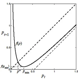
where > 0 is the constant speed of adjustment in the tâtonnement process. With this speci…cation, the function f (p) in the right-hand side of Eq. (3) has a minimum at pmin =
p
y0 and both a vertical and an oblique asymptote,
Fig. 1. The graph of the function f (p) and determination of the equilibrium price
To ensure that the adjustment process in Eq. (3) is well de…ned for all values of the price, it must be the case that f (p) is positive for all p, a requirement which is guaranteed if f (pmin) is positive, which requires
4 > [(1 ) x0] 2 y0 = pmin p !2 = K (5)
The constant K plays a crucial role in the analysis of the dynamics of the relative price generated by the present simple pure exchange model. Mukherji, in order to concentrate attention on this parameter, carries out most of his analysis for …xed values of all parameters but . The values he chooses are such that (1 ) x0 = 6and y0 = 1, and therefore K = 36 . For this special
case, which we will also assume to hold in all analysis and simulations which follow, he shows (1999, p. 745, Claims 2-3; cfr. also Day 1994, p. 200) that (i ) the equilibrium is locally stable for 0 < K < 2;4 (ii ) there exists a stable
2-cycle for 2 < K < 2:5; and (iii ) as K crosses the value of 2:5 a stable 4-cycle may exist, etc. in a route to chaos.5 These features of the dynamics of the
relative price are shown in the bifurcation diagram of Fig. 2, where K is used as the bifurcation parameter. As it is possible to grasp from this …gure, for
4 Actually, we can say something more about this. From (5) it follows that K can
be taken as a measure of the distance between pmin and p . When K = 1, pmin= p
and f0(pmin) = f0(p ) = 1 K = 0. In this case the equilibrium is superstable,
i.e., such that perturbations from it decay really fast. For other values of K in the stability interval, the convergence is slower, either monotonic, for values of K between 0 and 1 such that p > pmin, or cyclical, for values of K between 1 and 2
such that p < pmin.
5 Mukherji (ibid., Claims 4-5, pp. 745-748) also shows that the map exhibits
topo-logical chaos for K 2 (3:0; 3:6) and ergodic chaos for K = 25=9 and K ' 3:23 (the latter being a value in the interval (3:0; 3:6)).
0 0.5 1 1.5 2 2.5 3 3.5 4 0 2 4 6 8 10 K p*
Fig. 2. Bifurcation diagram of the pure exchange model map
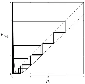
0 1 2 3 4 0 1 2 3 4 pt p t+1
Fig. 3. A trajectory for K = 4, with arbitrarily large values of the price, although not diverging
K = 4 the chaotic attractor becomes unbounded from above, although not diverging. This is due to a so-called contact bifurcation which …nds its origin in the fact that, as shown in Fig. 3, for K = 4 there is a contact between the critical point f (pmin)and the point pt= 0 at which the map (3) is not de…ned
(see Bischi et al. 2000). Apart from this special case, it is in general true that discrete-time tâtonnement mechanisms allow big irregular jumps of the price, which persist in time and are such that the equilibrium relative price is never reached. Two examples of dynamics of this type for values of K in the chaotic interval are illustrated in Fig. 4.
0 50 100 150 200 0 0.5 1 1.5 t pt (i) 0 50 100 150 200 0 5 10 15 t pt (ii)
Fig. 4. Two examples of chaotic dynamics of the price when (i ) K = 3:24 and (ii ) K = 3:9
In all cases like this, in which the relative price adjustment mechanism chosen by the auctioneer is not e¤ective in determining the equilibrium price of the good, transactions do not take place. Thus, the interesting question arises as to whether the auctioneer may use an alternative adjustment mechanism such as to guarantee convergence to the equilibrium price or, at least, to a price close to it. The rest of the paper is devoted to an attempt to answer this question.
3 A modi…ed pure exchange model with bounded price variations
In the literature on discrete-time tâtonnement with cautious price adjustment we have brie‡y referred to in the Introduction, the pure exchange model has been modi…ed by assuming a piecewise price adjustment mechanism such that the iterative process described by Eq. (3) of the original model holds over some middle range, but is restricted by a …xed maximal rate of increase or decrease of the price. The main result that is reached on the basis of this assumption is that any type of price dynamics, be it periodic or chaotic, is constrained in a neighborhood of the equilibrium price as time goes to in…nity (see, for exam-ple, Weddepohl 1995, p. 298). The stability properties of the latter, however, remain unchanged and therefore the price path does not actually converge to it.
In this section we follow a di¤erent strategy which consists in assuming that the auctioneer uses a smooth, rather than piecewise, nonlinear adjustment mechanism of the price, with an upper and a lower bound determined by two
parameters (let us say a and b) which – in contrast to what is assumed in previous literature –are not …xed, but are under her/his control. Our purpose is to show that, acting on one or the other (or on both) of these two parameters, s/he can not only restrict the dynamics of the price to a neighborhood of the equilibrium price, as was the case in the contributions we have mentioned above, but can even further control and stabilize it in a sense that will soon become clear.
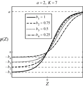
The idea we have in mind can be explored at its best by choosing in the discrete-time tâtonnement process (3), the following functional form for the function ' (Z (p)) (see Fig. 5):6
' (Z (p)) = (Z (p)) = a + b
a exp ( Z (p)) + b 1
!
b (6)
where a and b are strictly positive.7
A brief exploration of the properties of the function (Z (p)) will clarify what kind of consequences for the price dynamics we can expect:
i ) it is equal to zero at the origin of the axes: (0) = 0
ii ) it is an increasing function for all values of the excess demand: d
dZ =
0(Z) > 0 8Z
6 Any reader interested in nonlinear economic dynamics will recognize this
speci-…cation of a sigmoid-shaped function as the one used by Allen (1967, pp. 380-381) in his textbook on macroeconomic theory to represent Goodwin’s (1951a) nonlinear accelerator. We should also stress that a similar speci…cation for the reaction of price to excess demand is assumed to hold in the tâtonnement process formalized in Goeree et al (1998, p. 400). In their example, however, the two asymptotic values of price changes for excess demand going to 1 are numerically …xed and therefore the e¤ects of their control by the auctioneer cannot be discussed. On the contrary, as we will see, this type of analysis will be a basic ingredient of our study of the dynamics generated by the modi…ed model of this Section.
7 The reason for this requirement is that when a and/or b are equal to zero, equation
(3) with the speci…cation of ' (Z) given in (6) no longer describes a dynamic process: the price would remain for ever at its initial value, whether this is or is not the equilibrium price. We thank an anonymous referee who, thanks to her/his comment regarding the upper and lower limits to price dynamics, has led us to deepen and clarify this issue.
0 0 Z ψ(Z) a = 2, K = 7 a - b1 - b2 - b3 - b4 b1 = 1 b2 = 0.75 b3 = 0.5 b4 = 0.25
Fig. 5. A few examples of graphs of the function (Z) for di¤erent values of the parameter b
iii ) it has both a lower and an upper asymptotic bound such that: lim
Z! 1 (Z) = b < 0
lim
Z!+1 (Z) = a > 0
iv ) it has a positive slope at the origin of the axis that increases (decreases) as one or both of the two bounds becomes less (more) stringent:
0(0) = ab a + b > 0 such that: d 0(0) da = b a + b !2 > 0, d 0(0) db = a a + b 2 > 0
In short, our smooth adjustment mechanism is such as to preserve the sorting coming from excess demand and, at the same time, to impose bounds to price changes. As highlighted by property iv ), the existence of these bounds in‡uences the auctioneer’s behavior also at, and in the neighborhood of, the equilibrium and this appears very reasonable. It simply means that, even when the bounds are not binding, the more stringent they are, or just one of them is, the more cautiously the auctioneer adjusts the price in response to excess demand.
0 0.1 0.2 0.3 0.4 0.5 0.6 0.7 0.8 0.9 1 0 0.1 0.2 0.3 0.4 0.5 0.6 0.7 0.8 0.9 1 pt p t+1 a = 2, K = 7 g(pt) b = 1 b = 0.75 b = 0.5 b = 0.25
Fig. 6. A few examples of graphs of the function g(p) for di¤erent values of the parameter b
becomes (see Fig. 6):8
pt+1 = pt+ a + b a exp ( ( y0=pt) + (1 ) x0) + b 1 ! b = g (pt) (7)
In order to make easier the comparison with Mukherji’s results presented in Sect. 2, in Fig. 6 and in all the numerical analysis which follows we use the same …xed values for all parameters except = K=36and study what happens to the dynamics generated by the model when K is varied. For our modi…ed model, it will be in addition particularly relevant to concentrate on the e¤ects on the price dynamics of variations of the two parameters a and b, which are also under the control of the auctioneer.
4 Dynamic analysis of the modi…ed model
Our purpose in this Section is to show that the use by the auctioneer in the tâtonnement process of the sigmoid-shaped function described in Eq. (6) implies important qualitative changes for the relative price dynamics, both
8 To appreciate fully the di¤erence between our formulation and Mukherji’s one, it
is crucial to note that the vertical asymptote of the function f (p) of Fig. 1 is now replaced by a local maximum of the function g (p). The consequences of this will become clear in the discussion which follows. In a few words, we have now a ‘ceiling’ to the dynamics of price, which is endogenously generated by the formulation we have chosen for the function (Z (p)).
at a local and a global level. For reasons of clarity, in what follows we will consider the two levels separately.
4.1 Local analytical results
Given the properties of the function ( ), it is an easy task to show that the map of the modi…ed model we are now considering has the same equilib-rium p of the original model, but with di¤erent stability properties. This is summarized in the following two propositions.
Proposition 1 The dynamic map (7) has the same unique …xed point given by the equilibrium price p de…ned in (2).
Proof. A …xed point of (7) is de…ned by:
p = p + a + b a exp ( ( y0=p) + (1 ) x0) + b 1 ! b = g (p) which requires: a + b a exp ( ( y0=p) + (1 ) x0) + b 1 = 0 or a + b = a exp y0 p + (1 ) x0 ! + b i.e.: exp y0 p + (1 ) x0 ! = 1 i.e.: y0 p + (1 ) x0 = 0 from which: p = p = y0 (1 ) x0
This result, which shows the consistency of the two models in that they have the same unique equilibrium price, gives more meaning to their comparison. The following second proposition contains results about its local stability. Proposition 2 The stability condition for the unique …xed point of the dy-namic map (7) is given by
K 2 0; 2 1 a +
1
A 2-period bifurcation occurs at K = K1; hence, a 2-period locally stable cycle
exists if K 2 (K1; K1+ ), for all su¢ ciently small.
Proof. To derive condition (8), we …rst notice that at p , we have: g0(p ) = 1 ab (a + b) y0 (p )2 exp ( (by0=p ) + (1 ) x0) [a exp ( (by0=p ) + (1 ) x0) + b] 2 = 1 ab (a + b) [(1 ) x0] 2 y0 1 (a + b)2 = 1 abK a + b
Thus, the local stability condition,
jg0(p )j < 1 becomes:
1 abK
a + b < 1 which reduces to:
0 < abK a + b < 2 from which: 0 < K < 2 a + b ab ! = 2 1 a + 1 b = K1
The dynamic map (7) satis…es all canonical conditions required for a period doubling bifurcation at K = K1 (see, e.g., Hale and Koçak, 1991). Indeed,
when K = K1, p is a non-hyperbolic point, whereas when 0 < K < K1 it
is an attracting …xed point. Finally, p becomes repelling when K > K1 and
such that a locally attracting 2-period cycle emerges for K 2 (K1; K1+ ),
with su¢ ciently small.
Proposition 2 implies that the choice by the auctioneer of the functional form for the tâtonnement process given in Eq. (7) stabilizes the dynamics of the model. This can be fully appreciated by having a look at the bifurcation di-agram in Fig. 7, where we have chosen values for the parameters a and b such that the …rst period-doubling bifurcation occurs for K = K1 = 2 as in
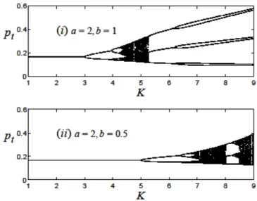
Mukherji’s example. Fixing the value of a at 2, we know from (8) that this happens when the parameter b is also equal to 2. The …gure clearly shows that after this …rst period-doubling bifurcation, the emerging 2-cycle remains sta-ble for a much larger interval of values of the parameter K than in Mukherji’s model. Moreover, the bifurcation diagrams of Fig. 8(i ), where b = 1, and Fig. 8(ii ), where b = 0:5, give evidence that this is the more true, the lower the value the auctioneer chooses for b: with regard to the …rst period-doubling bifurcation, for example, we see that it occurs for higher values of K, namely, K = 3 in Fig. 8(i ), where b = 1, and K = 5 in Fig. 8(ii ), where b = 0:5. In
Fig. 7. Bifurcation diagram of the model map with a = b = 2 such that K1 = 2 as
in Mukherji’s example
Fig. 8. Two examples of bifurcation diagram of the model map with (i ) a = 2, b = 1 and (ii ) a = 2, b = 0:5
short, although the period-doubling route to chaos is preserved, the sequence of bifurcations turns out to be moved forward.
4.2 Global numerical results
In this subsection, we perform further numerical simulations of the modi…ed model which extend and notably enhance our understanding of the dynamics it generates. The global dynamics features they are able to illustrate are of three di¤erent types.
First of all, they clearly show (see Fig. 9) that there is a contraction of the absorbing interval as the parameter b is decreased by the auctioneer.9 This
0 0.1 0.2 0.3 0.4 0.5 0.6 0 0.1 0.2 0.3 0.4 0.5 0.6 a = 2 b = 1 K = 9 (i) pt p t+1 0 0.1 0.2 0.3 0.4 0.5 0.6 0 0.1 0.2 0.3 0.4 0.5 0.6 a = 2 b = 0.5 K = 9 (ii) pt p t+1
Fig. 9. Contraction of the absorbing interval as b is decreased from (i ) b = 1 to (ii ) b = 0:5
feature is clear evidence in favor of a positive answer to Mukherji’s query about whether it is possible to control the tâtonnement process in such a way that the price, even if it does not converge to its equilibrium level, stays forever at least close to it. In our simple example, with …xed values for a, K, (1 ) x0
and y0, the auctioneer can easily attain this target if, during the tâtonnement
process, s/he makes more bounding the upper constraint to price variation.
Second, using the price adjustment mechanism formalized in (7), the auction-eer is also able to reduce the complexity of the price dynamics. This point can be easily understood by having a look at the value the derivative of the map (7) takes at the …xed point, namely:
g0(p ) = 1 ab a + b
!
K
where the second term in the right-hand side is increasing in both a and b. Thus, given a su¢ ciently high value of K (implying a high degree of dynamic complexity), it is always possible to …nd values of a or b such that the derivative is in the stability interval, i.e., such that g0(p )2 ( 1; 1). An example of the
reduction in the complexity of the attractor that follows from a reduction of b is shown in Fig. 10. We start, in Fig. 10(i ), from a combination of parameters such that the dynamics of the process is chaotic and check what happens when, all the other parameters remaining unchanged, the value of b is decreased. As shown in Fig. 10(ii ), in this case, the reduction of b from 1 to 0:75 drastically reduces the complexity of the attractor, which becomes a 2-cycle. Then, as (1997). In short, we can de…ne it as that interval to which the dynamics generated by our equation will always belong: starting from any initial condition, the dynamics will enter this interval in a …nite number of iterations and will never escape it.
0 0.1 0.2 0.3 0.4 0 0.1 0.2 0.3 0.4 pt p t+1 a = 2 b = 1 K = 4.5 (i) 0 0.1 0.2 0.3 0.4 0 0.1 0.2 0.3 0.4 pt p t+1 a = 2 b = 0.75 K = 4.5 (ii) 0 0.1 0.2 0.3 0.4 0 0.1 0.2 0.3 0.4 pt p t+1 a = 2 b = 0.5 K = 4.5 (iii)
Fig. 10. An example of reduction of the complexity of the attractor when K = 4:5 from (i ) a chaotic attractor to (ii ) a 2-cycle and (iii ) a …xed point
0 20 40 60 0 0.15 0.3 t pt a = 2, b = 1, K = 4.5 0 20 40 60 0 0.15 0.3 t pt a = 2, b = 0.75, K = 4.5 0 20 40 60 0 0.15 0.3 t pt a = 2, b = 0.5, K = 4.5
Fig. 11. The price dynamics for the same three cases as in Fig. 10
shown in Fig. 10(iii ), it is particularly worth noting that a further reduction to b = 0:5 transforms the latter into a …xed point (see also Fig. 11, where the same three cases are shown as versus time trajectories of the price).
mean-0 0.2 0.4 0.6 0.8 1 1.2 1.4 0 0.2 0.4 0.6 0.8 1 1.2 1.4 a = 2 b = 3.1 K = 4 (i) pt p t+1 0 0.2 0.4 0.6 0.8 1 1.2 1.4 0 0.2 0.4 0.6 0.8 1 1.2 1.4 a = 2 b = 1 K = 11.1 (ii) pt p t+1 0 0.2 0.4 0.6 0.8 1 1.2 1.4 0 0.2 0.4 0.6 0.8 1 1.2 1.4 a = 2 b = 0.5 K = 21.5 (iii) pt p t+1
Fig. 12. The graph of the function g(p) for di¤erent values of b and K ingful dynamics, it is required that K < 4 or, equivalently, < 0:111, in our example the intervals of admissible values of K and become larger as b is decreased. This property is shown in Fig. 12 where we start, in Fig. 12(i )), with the case in which the maximum admissible value of K is approximately equal to 4 as in Mukherji’s paper. Fixing a = 2 as in all other numerical sim-ulations in the paper, this turns out to be the case when b = 3:1. Then, Figs. 12(ii ) and 12(iii ) clearly show that, leaving the parameter a unchanged, this value increases to K ' 11:1 ( ' 0:308) when b = 1 and becomes as high as K = 21:5 ( ' 0:597) when b = 0:5.
5 Conclusions
In this paper we have carried out a simple exercise with the purpose of showing that it is possible to give a positive answer to Mukherji’s query about the e¤ectiveness of the tâtonnement process in discrete time. We have indeed been able to show that the auctioneer, by using a nonlinear price adjustment mechanism like (7) – such that the intensity of price variations during the tâtonnement process is positive and almost constant over some middle range of (absolute) values of excess demand but goes to zero at either extreme –is able not only to constrain the dynamics of the relative price in a neighborhood of its equilibrium level as small as s/he wishes, but even to fully stabilize it.
We believe that the theoretical relevance of this result, at length pursued in the literature, is beyond question. In addition, we believe that the price adjustment mechanism we have suggested could …nd interesting application in those real-world markets in which auction mechanisms play a role. Most obvious candidates for this are the large number of …nancial markets in which the price formation mechanism is of the tâtonnement type. For all these cases, the results we have obtained may shed light on potential mechanisms for price restraint. We leave this question open for future research.
Acknowledgements
Previous versions of the paper were presented at the 11th Workshop on Opti-mal Control, Dynamic Games and Nonlinear Dynamics, CenDEF, University of Amsterdam, Amsterdam, 31 May- 2 June 2010, at the MDEF 2010 (Modelli Dinamici in Economia e Finanza) Conference, University of Urbino, Urbino, Italy, 23-25 September 2010, at the NED11-7th International Conference on Nonlinear Economic Dynamics, Technical University of Cartagena, Cartagena, Spain, 1- 3 June 2011, and in a seminar at the Department of Economics and Management of the University of Trento, Trento, Italy, 30 November 2011. We thank all participants for their useful comments and suggestions. The remain-ing errors and shortcomremain-ings are our responsibility.
References
[1] Abraham R.H., Gardini L., Mira C. (1997). Chaos in Discrete Dynamical Systems. A Visual Introduction in 2 Dimensions. Springer-Verlag, New York.
[2] Allen R.G.D. (1967). Macro-Economic Theory. A Mathematical Treatment. Macmillan, London.
[3] Arrow K.J., Hurwicz L. (1958). On the stability of the competitive equilibrium, I. Econometrica 26, 522-552.
[4] Bala V., Majumdar M. (1992). Chaotic tatonnement. Economic Theory 2, 437-445.
[5] Bala V., Majumdar M., Mitra T. (1998). A note on controlling a chaotic tatonnement. Journal of Economic Behavior and Organization 33, 411-420.
[6] Bischi G.I., Mira C., Gardini L. (2000). Unbounded sets of attraction. International Journal of Bifurcation and Chaos 10, 1437-1469.
[7] Corron N.J., Pethel S.D., Hopper B.A. (2000). Controlling chaos with simple limiters. Physical Review Letters 84, 3835-3838.
[8] Day R.H. (1994). Complex Economic Dynamics. Vol. I: An Introduction to Dynamical Systems and Market Mechanisms. The MIT Press, Cambridge, MA. [9] Day R.H., Pianigiani G. (1991). Statistical dynamics and economics. Journal
of Economic Behavior and Organization 16, 37-83.
[10] Goeree J.K., Hommes C.H., Weddepohl C. (1998). Stability and complex dynamics in a discrete tâtonnement model. Journal of Economic Behavior and Organization 33, 395-420.
[11] Goodwin R.M. (1951a). The nonlinear accelerator and the persistence of business cycles. Econometrica 19, 1-16.
[12] Goodwin R.M. (1951b). Iteration, automatic computers, and economic dynamics. Metroeconomica 3, 1-7.
[13] Hale J.K., Koçak H. (1991). Dynamics and Bifurcations. Springer Verlag, New York.
[14] He X.-Z., Westerho¤ F.H. (2005). Commodity markets, price limiters and speculative price dynamics. Journal of Economic Dynamics and Control 29, 1577-1596.
[15] Kaizoji T. (1994). Multiple equilibria and chaotic tâtonnement: Applications of the Yamaguti-Matano theorem. Journal of Economic Behavior and Organization 24, 357-362.
[16] Lesourne J., Orléan A., Walliser B. (2006). Evolutionary Microeconomics. Springer Verlag, Berlin.
[17] Morishima M. (1996). Walras’ own theory of tatonnement [partly written in 1958]. In: Morishima M., Dynamic Economic Theory. Cambridge University Press, Cambridge, pp. 196-206.
[18] Morishima M. (1977). Walras’ Economics. A Pure Theory of Capital and Money. Cambridge University Press, Cambridge.
[19] Mukherji A. (1999). A simple example of complex dynamics. Economic Theory 14, 741-749.
[20] Saari D.G. (1985). Iterative price mechanisms. Econometrica 53, 1117-1131. [21] Saari D.G. (1991). Erratic behavior in economic models. Journal of Economic
Behavior and Organization 16, 3-35.
[22] Samuelson P.A. (1941). The stability of equilibrium: comparative statics and dynamics. Econometrica 9, 97-120.
[23] Samuelson P.A. (1947). Foundations of Economic Analysis, Enlarged edn., 1983. Harvard University Press, Cambridge, MA.
[24] Tuinstra J. (2002). Nonlinear dynamics and the stability of competitive equilibria. In: Hommes C.H., Ramer R., Withagen C.A. (eds), Equilibrium, Markets and Dynamics. Essays in Honour of Claus Weddepohl. Springer Verlag, Berlin, pp. 299-344.
[25] Uzawa H. (1960). Walras’ tâtonnement in the theory of exchange. Review of Economic Studies 27, 182-194.
[26] Weddepohl C. (1994). Erratic dynamics in a restricted tatonnement process with two and three goods. In: Grasman J., van Straten G. (eds), Predictability and Nonlinear Modelling in Natural Sciences and Economics. Kluwer, Dordrecht, pp. 610-621.
[27] Weddepohl C. (1995). A cautious price adjustment mechanism: chaotic behavior. Journal of Economic Behavior and Organization 27. 293-300