UNIVERSITA’ DEGLI STUDI DI MESSINA
Department of EconomicsPhD in: ECONOMICS, MANAGEMENT AND STATISTICS
XXXII Cycle
Coordinator: Prof. Edoardo OTRANTO
____________________________________________________________________________
On modelling the multivariate Realized
Kernel financial time series
PhD Student: Tutor:
Dott.ssa Alessandra COSTA Illustrious Professor
Edoardo OTRANTO
____________________________________________________________________________
3
Sommario
Introduction and Objectives of the Work ... 6
A Survey of Realized Volatility and High Frequency Data ... 8
1.Introduction ... 9
1.2 Volatility ... 10
1.2.1 Fat tails... 11
1.2.2 Volatility Clustering... 11
1.2.3 Leverage effect ... 11
1.3 High Frequency Data ... 12
1.3.1 Asynchronous trading ... 13
1.3.2 Bid-ask spread ... 13
1.3.3 Univariate Setting: Quadratic Variation and Integrated Variance ... 14
1.3.4 Realized Variance (RV) Estimator ... 16
1.3.5 Sampling frequency and Market Microstructure Noise... 17
1.3.6 Kernel-Based Estimator ... 19
1.3.7 Multivariate Setting: Quadratic Covariation ... 20
1.3.8 CholCov Estimator ... 21
A Class of Multivariate Models for Realized Conditional Variance and Covariance Matrices ... 24
2.1 Introduction ... 25
2.2 General Framework... 27
2.1 Univariate Volatility Modelling ... 28
2.2 DCC-CAW-MEM ... 29
2.3 Alternative parametrizations: BEKK dynamics ... 34
2.4 Covariance Targeting ... 35
2.5 Additional models ... 37
2.6 Estimation Procedures Concluding Remarks ... 38
Evidence from Real Data ... 40
3.1 Dataset... 41
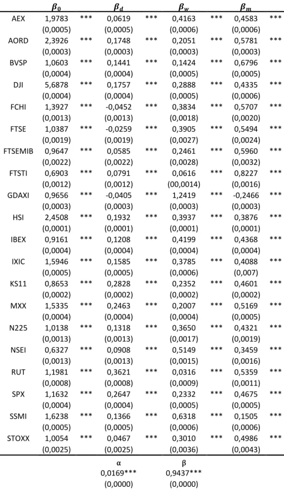
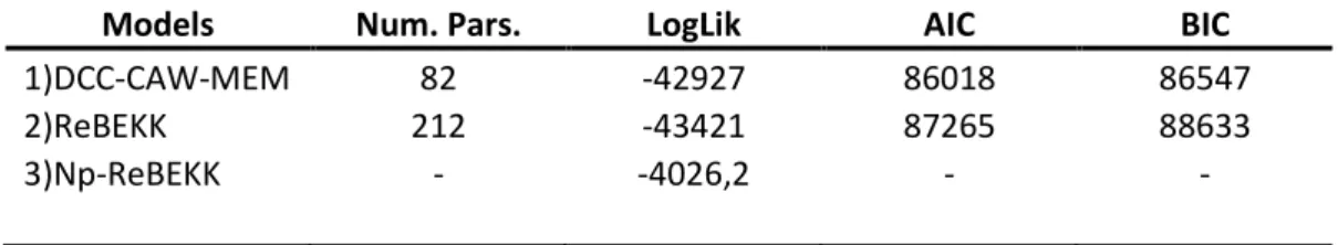
3.2 Full sample results ... 47
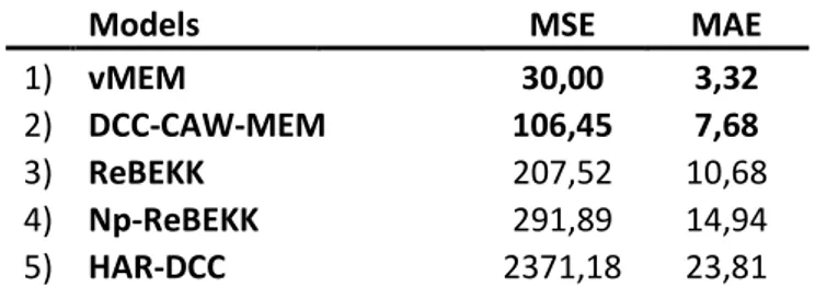
3.3 Forecasting results ... 57
3.3.1 Model Confidence Set ... 57
Conclusions ... 60
Appendix A ... 63
4
a.2) Correlation Matrix ... 63
Appendix B ... 85
The Wishart distribution ... 85
Overview of models ... 87
6
Introduction and Objectives of the Work
It is widely known that financial time series are characterized by very complex patterns and dynamics, that have to be accounting in estimation and forecasting analysis. Multivariate GARCH models have been and continue to be the most widely used time series models, both with parametric and non-parametric specifications: major examples are BEKK of Engle and Kroner (1995), the CCC of Bollerslev (1990) and the DCC of Engle (2002). Those models allow for volatility and correlations to change over time, and one of their main advantage is their easily implementation in many areas. More recently, the growing availability of high frequency data allows the development of different ex-post unbiased estimators of daily and intraday volatility, and this stimulated the development of specific models directly fitted on realized measures. Thus, although many multivariate variants of existing models could be applied on realized measures too, other specific models were adopted. Just to mention a few, the Realized GARCH of Hansen, Huang and Shek (2010), the Multiplicative Error Model of Engle (2002) and HEAVY models. Moreover, when multiple assets are involved, other issues arise (asynchronous trading and microstructure noise). Previous considerations underline the need for parametrizations and models able to guarantee the positiveness of variance covariance matrix at each point in time. As a natural consequence, the best choice is to adopt a Wishart distribution that automatically generates PSD matrices. Secondly, since the number of parameters to estimate clearly are proportionally to the number of assets included in the analysis, the estimation process could become infeasible. Thus, to overcome the curse-of-dimensionality problem that could arise, it is necessary to define several constraints in the models to estimate, however guaranteeing a high level of flexibility in the model parametrization. In view of this background, this thesis is structured as follow:
1. Chapter 1 introduces some preliminary concepts about volatility and its stylized facts, high frequency data and realized measures;
2. Chapter 2 presents a class of models inspired by the consideration of simplicity, feasibility and computational speed in high dimensional environment.
7
Among them, a new parametrization that combine a multiplicative structure with dynamic correlations and variances, the DCC-CAW-MEM, directly fitted on the realized variance covariances matrices. After exploiting its characteristics, its estimation process (ML approach and QML interpretation), we also consider other parametrizations that have been found to be fit well in high dimensional context. Some of them rely on the same multiplicative error structure of DCC-CAW-MEM and require the maximization of the same likelihood function, even if each of them presents a different structure and has a different degree of flexibility.
3. Chapter 3 shows the empirical application of all the models discussed in the previous chapter, both in the in-sample and out of sample scenarios.
8
Chapter 1
A Survey of Realized Volatility and
High Frequency Data
Abstract
In this chapter, I briefly review the concept of volatility, its main features and problems that can arise during its measurement. Then I introduce the topic of high frequency (HF) data, by focusing on the relationship between HF data and the microstructure noise. Consequently, I present the most common ex-post volatility estimator, the Realized Variance (RV) (Andersen et al, 2003). Then I extend the concept to the multivariate context, by considering more than two assets through the introduction of realized covariance estimators. Both in the univariate and in the multivariate setting, I will start from the introduction of a diffusion continuous time framework of analysis (Brownian motion).
9
1.Introduction
Volatility represents an interesting topic in financial time series, because it plays a central role in different area1. Although volatility is, in principle, a clear concept, its statistical treatment is not simple, because it is a latent variable which has to be estimated. This explains why it has received a lot of attention in literature, that has moved into two directions: the development of new models with richer formulations, that should result in higher estimation and forecasting performances, and a better classification of the existing models. With respect to the model development process, models range from the basic historical volatility ones (random walk, moving average, etc.) to the more complex and well-known ARCH ang GARCH models and their extension. Comprehensive reviews of literature can be found in Bauwens et al (2006) and in Silvennoinen and Terasvirta (2009). Referring to ranking among models, there is no consensus about which class of model performs better, and such conclusion comes from a set of mixed literature findings, even if many GARCH models still perform well in many applications. More recently, the availability of intraday data has led to the rise of a growing interest in new ex-post volatility measures. In fact, realized volatility measures solve some issues of the traditional methods that rely on daily data (usually, daily squared returns).
High frequency data (HF) introduces the possibility to add further assumptions for multivariate process high frequency variables. The availability of a great amount of information has led to an increase in the accuracy of the forecasts and to an advantage over traditional low frequency methodologies, which require data over a long period
1 Poon and Granger (2003) stated that volatility forecasting is an important tool in financial risk management, while Andersen et al (2003) found three preliminarily applications of it: a) pure forecasting applications; 2) financial risk management for banks and trading houses; 3) generic applications outside financial field, but related to real economy. Relative to the last application of volatility forecasting, a lot of evidence can be found in literature. Just to mention a few, Coshall et al (2009) applied univariate volatility models to the UK tourism demand to the country’s most popular international destinations, using twelve quarterly time series collected from the UK Office for National Statistics over the period 1977-2008, while Moran et al (2017) used multivariate time series analysis for modelling daily mean-mortality series of intensive car society units (ICUs) from Australian adult patient database, also confirming the validity of classical financial time series patterns. Moreover, Escribano et al (2018) modelled the volatility of electricity prices of Nord Pool Spot AS through a multiplicative component log-GARCH-X. Obviously, other relevant examples can be founded, but the selected ones help to evidence how much volatility model techniques are widely used in all interesting areas.
10
of time. At the same time, there could be gains from financial processes and from the successful management of risks and trading costs.
Moreover, one of the most important aspect when we talk about high frequency data is the sampling frequency. Even if using low frequency data measure could lead to imprecise estimates and forecast, computing the estimates to a very high frequency introduce some biases in the estimation itself, due to the contamination of microstructure noise. This has led many researchers to focus their research on ex-post estimation of daily variance and covariance of assets, using information based on intra-daily price registrations and on the development of unbiased estimators and alternative approaches.
1.2 Volatility
In everyday language, volatility refers to the fluctuations observed in a certain phenomenon over time, while in economics it is used to describe the variability of a time series.
More formally, in financial economics, the term volatility is defined as the standard deviation of a continuous time process.
Depending on data availability and on the uses of model estimates, volatility models can be designed in discrete time or continuous time, even if it is clear that in many liquid financial markets, transactions take time at very short interval. As a consequence, it is natural to think about the priced and returns series of financial assets as arising through discrete observations from a continuous time diffusion process. Although many discrete models have been shown to be not consistent with the corresponding continuous modes, they are still used and preferred because of their flexibility in the estimation process. In this thesis I refer to volatility as the level of uncertainty associated to a financial asset, and it has been proved to be characterized by certain stylized facts, that are crucial for the correct specification of all the volatility models.
11
1.2.1 Fat tails
It is a well-known point that the distribution of financial time series normally exhibits fatter tails than the normal distribution. Assuming that the fourth order moment of a GARCH(1,1) exists, Bollerslev stated that many financial time series exhibit a kurtosis index greater than the standardized value of 3. Afterward, He and Terasvirta (1999) generalized the same results for the GARCH(p,q).
1.2.2 Volatility Clustering
Volatility clustering was firstly introduced by Mandelbrot (1963),who reported “… in other words large changes tend to be followed by large changes- of either sign- and small changes tend to be followed by small changes…”.
Lux and Marchesi (2000) attribute volatility clustering to the agent switching between fundamentalist and chartist strategies, while Kirchler and Huber (2007) suggested as source of volatility clustering the presence of heterogeneous information, and by assuming that traders learn from observed prices2.
As reported by Aldridge (2009) current high volatility does not typically revert to lower volatility levels instantaneously, but higher volatility typically persists for different periods (this is also known as ARCH or GARCH effect). Thus, clustering is strictly related to the persistence or long memory of volatility. Especially in high frequency context, there is a lot of evidence of a near unit root in the conditional variances. Bollerslev (1998) suggests to use a visual inspection for determining the time series properties of volatility, by referring both to the absolute returns and square returns in the correlogram analysis.
1.2.3 Leverage effect
The leverage effect, also known as volatility asymmetry (Black, 1972), typically refers to the negative correlation between volatility and past returns. More precisely, this
2 For further details, see Smith, V. L. (1982), Markets As Economizers Of Information: Experimental Examination Of The “Hayek Hypothesis”. Economic Inquiry, 20: 165-179. doi:10.1111/j.1465-7295.1982.tb01149.x
12
effect implies that an increase in asset prices is accompanied by declining volatility, and it is asymmetric, so a moderate reduction of an asset price determines a larger increase of financial volatility.
1.3 High Frequency Data
In the last years, the growing availability of high frequency data has represented one of the most attractive field of research in financial econometrics. With financial and technological developments, the possibility to have tick by tick data has increased the interest of researchers in their management, to better understand the structure of financial markets.
Andersen et al (2003) highlighted the improvements high frequency data produces in terms of predictive performances respect to the standard procedures that rely on daily data alone. This, in principle, led to obvious advantages in financial applications, especially in situation where prices arise from a continued time diffusion process. In other words, we could expect that more observation we have, the more precise the estimations will be. Unfortunately, some problems arise. It is obvious that except for most liquid assets, the continuous price is not available, and this implies the existence of a measurement error that must be taken into account. Secondly, when the sampling frequency increases, it also will increase the probability of occurrence of spurious correlations. Therefore, in practical applications, we have to deal with a trade-off between accuracy of estimates and forecasts and measurement errors, in order to reduce bias and distortions in statistical inference. In this section I analyze the trade-off between microstructure noise and sampling scheme, by introducing some sources of microstructure noise and analyzing the different sampling schemes available in financial literature.
Falkenberry (2002) synthetized the nature of the problems arising from the creation and the management of high frequency database. Among others (different nature of error types, intraday seasonal patterns in tick frequency, treatment of time, etc.), the main sources of microstructure noise are:
13
Asynchronous nature of tick data; Bid-ask bounce.
1.3.1 Asynchronous trading
In an ideal market, trading is synchronized, that means that all the buyers and sellers meet at the same time and conclude transactions, whose prices are recorded in the same moment. In practice, this not happens, and transactions take place in different moments. The effect of non-synchronous trading has firstly been investigated by Atchison et al (1987), who examined its effect on autocorrelation among assets. The effects of asynchronous trading arise when time series are wrongly measured. Generally, reported daily returns only reflect the last trade that takes place. Such scenario means that, in high frequency context, one incorrectly assumes daily returns as an equally space time series over a 24-hours interval. Scholes and Williams (1977) demonstrated that this non synchronous trading induces lag cross correlations and lag serial cross correlations into returns. Most importantly, Tsay (2003) evidenced this effect in terms of portfolio construction, since it leads to biased correlations among assets and inaccuracy in assessing risks in management strategies.
1.3.2 Bid-ask spread
The bid-ask spread, often considered as trading cost, is due to the difference between the price at which the buyer wants to buy and the price at which the seller wants to sell.
Following Stoll (1989), the transaction cost from which bid-ask spread arises comes from under processing costs, inventory holding costs and adverse information costs. In fact, in order to maintain liquidity, many exchanges use market makers who stand ready to buy or sell whatever the public wishes to buy or to sell, but they usually buy at bid price and sell at higher ask price. As a convention among market makers, bid-ask spreads usually take few discrete values, while in practice the bid-bid-ask spread is time varying and related to both volume and volatility. Such result is due to transaction prices which are free to move between the ask and the bid, in a manner that they can
14
produce different log returns, even if the economic values of the assets is still the same. This scenario is known as bid-ask bounce, that is the bid-ask spread that introduce negative lag-1 serial correlation in asset returns, that has been exploited and modelled by Roll (1984).
1.3.3 Univariate Setting: Quadratic Variation and Integrated Variance
Now I am presenting the framework on which my analysis, in univariate setting, is based. As mentioned before, since many models have been formulated in a discrete time framework, it is natural to start from observation available at equally spaced discrete points in time. Let’s think to a discrete process
≡
ℎ = 1,2, . . . , where is assumed to arises from a continuous process, with the following conditional moments (mean and variance)
ϻ | = |
and
ϭ | = | = − ϻ |
where is the set of information available at time t-1, that determines the differences between the conditional and unconditional moments.
As previously noted, most of the main applications in volatility modelling have been developed in the context of financial economics, thus it is natural to think about prices and returns. If we assume that p(t) is the univariate process of the logarithmic price evolving in the continuous time over a discrete internal [0,T], Back (1991) and Andersen et al (2003), and if the return process does not allow for arbitrage and a finite instantaneous mean, the asset price belongs than the log prices belong to the class of semi-martingale and it can be written as the sum of a drift component A(t) and a local martingale M:
= 0 + # + $
Moreover, the latter can be splitted in two components: a realization of a continuous process, ∆# and ∆$ and a jump component. With the initial assumption that ∆$ 0 ≡ # 0 ≡ 0
15
= 0 + #& + ∆# + $& + ∆$
This decomposition is useful for the qualitative characterization of the asset return process. Since the return over [t-h, t] is defined as − − ℎ , this implies that:
= + − ℎ = # + $
Similarly, we can refer to the multivariate case involving of returns, by the upper-case letter R.
Until now I have considered a discrete time framework but, as noted before, it is natural to think of prices and return arising from a continuous diffusion process in the form of:
' = ϻ ' + ϭ '(
ℎ ≥ 0 where ( is a Wiener process, ϻ is a finite variation stochastic process and ϭ is a strictly positive cadlàg and it is the instantaneous volatility of the process. From this characterization, it follows that over the interval [t-h, t] if we consider a unit variation, h=1, we get
= − − 1 = * ϻ + '+ + * ϭ + ' ( +
ℎ 0 ≤ + ≤ ≤ The similitudes between the discrete and continuous characterizations are clear: the conditional mean and variance process are replaced by the corresponding integrated realizations of means and variances. Because the variation of the diffusion path of martingale is not affected by the drift component, intuitively its evolution is related to the evolution of the coefficient ϭ.
Formally, the return variation is equal to the so-called quadratic variation: - = * ϭ
. + '+
The quadratic variation process could be approximated by cumulating cross products of high frequency returns. As noted by Andersen et al (2003), the quadratic variation is the main determinant of return covariance matrix, especially for shorter horizons, since the variation induced by genuine innovation, represented by the martingale component, locally is an order of magnitude larger than the return variation caused by changes in the conditional mean.
16
The diffusive sample path variation over [t-h, t] is also known as the integrated variance IV.
/ = * ϭ
. + '+
Under the simplifying assumptions of absence of microstructure noise and measurement error, the quadratic and integrated variation coincide.
1.3.4 Realized Variance (RV) Estimator
Given the previous characterization, the researchers developed different estimators of the integrated variance. The most widely used is the realized variance (RV) estimator. I firstly examine the ideal context in which the absence of measurement errors made ex post volatility became observable. Andersen et al. (2003) suggested to estimate the realized variance as the sum of squared intraday returns, sampled at sufficiently high frequency. Considering − ℎ + 0
1 a partition of t − h, t interval, thus the realized
variance will be defined as
4 = 5 6
.701− .8 9
.:
It has been shown to be an unbiased estimator of ex-ante volatility, and in case of absence of microstructure noise it is also an unbiased estimator of the integrated variance. Moreover, several authors refer to realized volatility as the square root of RV.
Many authors have started to individuate an appropriate framework for the estimation and the prediction of conditional variance of financial assets, in order to accommodate for the entire set of information in intraday data. Based on the results of Jacod and Protter (1998), Barndorff-Nielsen (2002) derived the asymptotic distribution of the realized variance as normal with zero mean and unit variance. As sampling frequency increases, the realized variance converges in probability to the quadratic variation (QV)
17
This is the formal link between RV and return quadratic variation, that directly follows from the theory of semi martingales and implies that as sampling frequency increases, RV provides a consistent measure of the IV. If this is true, in theory one could reduce the measurement error by increasing the sampling frequency. However, given the arguments introduce in Section 1.3, returns shouldn’t be sampled to often to avoid microstructure noise.
1.3.5 Sampling frequency and Market Microstructure Noise
As stated above, even if high frequency data represent a source of continuous information, there is a well-known bias between sampling frequency and microstructure noise.
Andersen et al. (2003) highlighted how much crucial is the choice of the sampling frequency, considering high frequency data on deutschmark and yen returns against the dollar. By simulated volatility signature at varies sampling intervals, they individuated as optimal the 20-minute return sampling interval (k=20), that contemporaneously measures the microstructural bias and the sampling error.
Aït-Sahalia et al. (2005) and Zhang et al. (2009) proved that RV is not a reliable estimator for the true variation of the returns in case of microstructure noise, since as sampling frequency increases, the noise becomes progressively more dominant. Consequently, literature recommends to use a realized variance estimator constructed by summing up intraday returns at some lower sampling frequency, usually 10, 15 or 20 minutes.
About this, it is possible to refer to the sparse sampling scheme, and it has been suggested by Andersen et al (2001). When sampling frequency is lower than the -1 min, sparse RV, 4 > will be:
4 > = 5 ,? > 1@A ?:
It has been shown that the bias due to the noise is reduced when ;> < ;, even if the total variance increases. Although sparse sampling tries reducing the microstructure noise in RV calculation, it potentially suffers from a loss of information and leads to a reduction in the efficiency of the estimator. For this reason, Bandi and Russel (2008) proposed to select the optimal sampling frequency by minimizing MSE (mean square
18
error). The authors presented a methodology similar to Bei et al. (2000), that is able to choose optimal sampling frequency by minimizing the expected square distance between the estimator (RV) and its theoretical counterpart (QV) as summarized by conditional MSE.
At the same time, Zhang et al. proposed an alternative method to benefit from using infrequently data. Instead of arbitrarily selecting a subsample, the authors suggested to select a number of sub-grids of the original grid of observation time C = ⋃F C E
F: , where C F ⋂ CH≭ Ø (when k ≭l) and the natural way to select the kth
subgrid is to start from F and then pick every kth sample point until Ƭ, that means: CF = K F , F 7F, F 7 F, … , F 71MFN
Given the realized volatility 4 F = ∑1?: ,? , Zhang et al. averaged the estimator, and then:
4 PQR = 1E 5 4 9F −;; 4 9PHH
F F:
Fixing T and using the observation within the interval [0,T] asymptotically as ; → ∞ and ; ES → ∞, ;F hasn’t to be the same across k, we could define we get
; = 1E 5 ;F
F F:
=; − E + 1E
The estimator is called Two Time Scales Estimator (TTSE), obtained through a combination of single grid and multiple grids.
Under the assumption of IID noise structure (the microstructure noise has zero mean and is IID random variable independent of the price process and the variance of T is O(1)), they showed that
; /V 4 WXY− / → 8\ − 2ℒ ] + \^ 9 _ 0,1
and the converge is stable in law. For equidistant sampling and regular allocation to grids, ^ = `
ab , the variance is equal to 8\ − 2 ] + \^ = 8\ − 2 ] +
\`ab` .
In their paper, Zhang et al. demonstrated that the optimal choice of c becomes: \cd = e12 ]b` f
19
As the authors pointed out, it is also possible to estimate c to minimize the actual asymptotic variance from data in the present time period, or 0 ≤ ≤ . With a bias-type adjustment, the estimator will be unbiased
4 Pg0 = e1 −;;f 4
The difference between the two estimators is of order h i; ;S j = h E .
Moreover, referring to the sample schemes, McAleer and Medeiros (2008) individuated four sampling schemes:
1. Calendar time sampling (CTS), where the intervals are equidistant in calendar time, that’s k?,1 =
1@ for all i.
2. The transaction time sampling (TrTS), where prices are recorder every n-th transaction;
3. Business time sampling (BTS), where the sampling times are chosen such that / ? = lm1@;
4. The tick time sampling (TkTS), where prices are recorder with each transaction.
As pointed out by Oomen (2006), the choices of both sampling and calendar schemes are crucial for modelling and forecasting. Oomen showed that from theorical and empirical analysis, transaction time sampling is superior to the common approach of CTS, and it leads to a better minimization in MSE of the realized variance, yielding more accurate variance estimates.
Furthermore, Griffin and Oomen (2008) proposed a comparison of the effect of tick time and transaction time sampling on RV calculations.
1.3.6 Kernel-Based Estimator
Motivated by the some of the issues mentioned before, in literature other estimators have been proposed for modeling the microstructure noise, such as the Kernel based estimators of QV, in presence of autocorrelation caused by microstructure noise.
20
Zhou (1996) was the first to use kernel function to deal with the problem of microstructure noise in high frequency data, proposing the following estimator:
4 n = 4 + 2 5 ; ; − E n F: opF Where opF = i 1
1 Fj ∑1 .0: ,0 ,07 , 4 is the all RV and E · is the Kernel function
and n is the sum of intraday observations used in RV computation.
Even if this estimator is unbiased, it is not consistent when we move to continuous. Extending Zhan’s work, Hansen and Lunde (2005) analyzed the implication of microstructure noise on RV estimates, and by using the Down Jones Industrial Average, they revealed some features of microstructure noise, with important implication for RV estimation.
Given the time dependency and the correlation with the returns of the efficient price, the authors introduced the 4 Yr estimator, that uses the first order autocorrelation to bias correct the RV. Starting from Zhou’s estimator of 1996, the authors derived its properties allowing for non-constant volatility and non-Gaussian microstructure noise. Afterwards they compared the two estimators, demonstrating that 4 Yr performs better, as summarized by a greater reduction of MSE.
1.3.7 Multivariate Setting: Quadratic Covariation
In this section I focus on the analysis of methodologies used for producing ex-post measures of the covariance between assets.
Before turning into the discussion about them, I have to introduce several assumptions about the underlying data generation process. As in the univariate setting, I focus on a continuous time diffusion model, supposing that I have n stocks whose log price process is ?. As evidenced in Section 1.3.3 the continuous model can be summarized as:
= * ϻ + '+ + * s + ' ( +
where ϻ is a m by 1 vector of drift process and s is the spot co-volatility, while W is a vector of the Brownian motion.
21
In this the quadratic variation can be defined using matrix notation, as: -t = u v 5w 0− 0 x w 0− 0 xy
Following advances in the realized co-volatility literature, we are interested in modelling and forecasting the daily ex-post covariation, through appropriate realized covariance estimators.
The most used estimator of quadratic covariation is the so-called Realized Covariance (RC), introduce in financial literature by Barndorff-Nielsen & Shephard (2004). The authors showed that, if we can observe the log price processes at discrete points in time over an interval [0,T], with T=1, and if we have j intraday observations, the RC estimator is the sum given in the definition of quadratic variation, so that:
4t = 5w 0− 0 xw 0 − 0 xy 1
0:
Also in this case, under the assumption of no microstructure noise, it has been shown that RC is an unbiased estimator of the variance covariance matrix z . Even in theory, the estimation will be simple, in practice some problems persist (asynchronous trading and microstructure noise).
1.3.8 CholCov Estimator
Since we rely on high frequency data, it is necessary to individuate an appropriate and consistent estimator of realized variance covariance matrix, by considering that in a multivariate setting, besides the accuracy of the estimator, the literature has extensively studied the need of a positive definite estimators3. Since our object of
interest is the spot covariance matrix over the unit interval /th = * z + ' +
{
3 For a complete survey about the estimation of both low and high dimensional covariance matrix and related estimation problems see Wei Biao Wu and Han Xiao (2011).
22
In this work for its computation, I will refer to Boudt et al. (2016) estimator, the CholCov, that has been found to be a consistent ex-post estimator of the variance covariance matrix, both to microstructure noise and asynchronous trading (after some refinement procedures). Starting from the ex-post covariation of log-prices, the estimator relies on a Cholesky decomposition4 of the spot covariance matrix into symmetric positive definite square matrices. By the Cholesky factorization, the spot covariance matrix z + can be decomposed into a lower triangular matrix | + with unit diagonal elements and a diagonal matrix } + , so that
z + = | + } + | + y
that means, with a matrix representation: | + = ~ 1 0 ⋯ 0 ℎ 1 … 0 ⋮ ⋮ ⋱ ⋮ ℎ1 0 ⋯ 1 ‚ ;k } + = ⎣ ⎢ ⎢ ⎡†0> † 0 ⋯ 0 > … 0 ⋮ ⋮ ⋱ ⋮ 0 0 ⋯ †gg > ⎦⎥ ⎥ ⎤
And, as reported by the authors, the link of each element of H and G matrices to the elements of the spot covariance matrix z + are represented by the following links:
†FF = zFF− 5 ℎFŠ†ŠŠ F Š: ℎFH = †1 HH‹zFH − 5 ℎFŠℎHŠ†ŠŠ F Š: Œ
The usefulness of this decomposition is the possibility to use as much data as possible and hold for any PSD matrix, that is true for the covariance matrix. Moreover, the authors demonstrated that its computational effort is compensated by an efficiency
4 To be more precise, the Cholesky decomposition has widely been used in the volatility context (see Chiriac and Voev (2011) and Palandri (2009).
23
gain. if compared to other robust estimators (think about the multivariate realized kernel of Barndorff-Nielsen et al. (2011)), even if in case of microstructure noise the authors suggest to better refine the estimation procedure, by using integrated variance robust estimators.
Realized variance covariances matrices used in the empirical application of Chapter 3 has been computed through the CholCov estimator, in order to obtain a series of PSD matrices as input of our estimates. Moreover, for better ensuring the reliability of the inferential results, some econometricians suggest to use a robust procedure for getting robust standard errors (lets’ think about the sandwich estimator or the Moore—Penrose pseudo-inverse, when the number of stocks is greater than the number of observations).
24
Chapter 2
A Class of Multivariate
Models for Realized
Conditional Variance and
Covariance Matrices
Abstract:
Starting from the Engles’s (1982) paper about ARCH model, many models have been developed in order to better modelling financial volatility and its stylized fats. Even if ARCH and GARCH models are still the most used models in many practical applications, recent attention has been devoted to the volatility measurement on the basis of ultra-high frequency data.
Despite the effectiveness of GARCH models, the new frontiers in analyzing volatility is represented by the Multiplicative Error Model, the MEM (Engle, 2002; Engle and Gallo, 2006; Brownlees et al., 2011), in which volatility is modelled as a product of a time-varying factor and a positive random variable, ensuring positiveness, without resorting to logs.
Moreover, in high frequency context, another task of great importance is the modelling of variance covariance matrix. Although the RC estimator introduced before, the new frontiers in financial literature are represented by dynamic parametrizations for time-varying daily variance covariances matrices. In this spirit we will refer to formulations consistent with dynamic conditional correlation typical of GARCH volatility models.
25
2.1 Introduction
Even if GARCH models were originally defined in a univariate setting, their formulations have been easily adapted to the multivariate context.
It is a well-known fact that financial time series are characterized by complex patterns and that an important role is played by the co-movements among assets. Thus, considering only financial modelling in univariate setting could led to a misspecification of the models, accounting for co-movements among assets has become a relevant topic in financial literature. In this field of research there has been a flourishing literature and many models have been developed. Multivariate GARCH models have been and still are the most widely used time series to correctly represent the covariance matrix. Let’s think about BEKK model of Baba, Engle, Kraft e Kronecker (1995), the Conditional Constant Correlation of Bollerslev (1986), the Dynamic Conditional Correlation of Engle (2002).
Moreover, respect to the traditional setting, when moving from univariate to multivariate framework of analysis, practitioners have to deal with two additional issues, that have been different exploited in research: the imposition of some additional restrictions and conditions to ensure the positiveness of the variance-covariance matrices.
To this regard, different distributional choices have been taken into consideration, in order to obtain a PSD variance covariance matrix, such as the exponential and the gamma distribution, and the multivariate Wishart distribution.
About the latter, one example is the Conditional Autoregressive Wishart (CAW) model of Golosnoy et al. (2012), where the realized variance covariance matrix has been modelled trough the combination of a Wishart distribution and a BEKK time-varying dynamics. In the same spirit, Bauwens et al. (2016) explored the potential benefits of combining high and low frequency data, in the spirit of the Midas Data Sampling (MIDAS) filter, by separately accounting the long run level of covolatilities and their short run dynamics, through CAW-MIDAS.
In addition, the HF data has increased the interest of researchers to model the series of realized covariances, that could be obtained by exploiting all the information available.
26
Thus, in this chapter I introduce the models used in the chapter 3, for the empirical application. Even if here the interest is not to offer a complete survey of the models, I will highlight the interesting features of each model used in the empirical study. Moreover, by combining some innovative key elements founded in the financial literature, I introduce a DCC-CAW-MEM model in high dimensional context. More precisely, I combined a consistent DCC-GARCH type parametrization with a vector Multiplicative Error Model (MEM) of Cipollini et al (2012), through a multivariate Wishart distribution. The time varying parametrization allowed to extract the co-movement among assets, by using all the information guaranteed by a high frequency multiplicative error structure. Moreover, the additional Wishart distribution allowed to use a Quasi Maximum Likelihood approach, that simplify the optimization.
Finally, before turning into discussion, it is important to note that in many practical applications, the multivariate modelling is translated into much simpler multiple univariate procedures, after appropriate series transformations. Moreover, instead of concentrating on univariate formulation, I will directly describe their multivariate extensions, that will be used in the empirical application in Chapter 3.
27
2.2 General Framework
The general framework proposed here is the one illustrated in the Section 1.3.7. For the model specification, let’s start from the Wishart distribution5. Suppose that t is a sequence of positive definite symmetric (PDS) realized covariance matrices of daily realized kernel volatility of n assets, conditioned on the available set of information . By assumption, the conditional distribution of t, given the past history of the
process , consisting of t for T ≤ t-1, follow a Wishart distribution: t | ̴ (1 T , Ž TS
where T is the degrees of freedom parameter and Ž TS is a PDS scale matrix of order ;.
From the properties of Wishart distribution6, it follows that: t | = 7 t = Ž
whit Ž the conditional covariance matrix, whose i,j-th element is the covariance between assets i and j.
The previous equations define the baseline CAW (Conditional Autoregressive Wishart) model with a time-varying scale matrix.
Our idea is to use a decomposition of the scale matrix Ž , in order to separately account for volatility and correlations. In the spirit of Bauwens, Storti and Violante (2012) and Bauwens, Braione and Storti (2016), I firstly decomposed the scale matrix in term of standard deviation and correlations, so that:
5 Several authors use the Wishart distribution, because it allows to model each element of the correlation matrix, when more than two elements vary and it guarantee positive definite draws. Gourieroux, Jasiak and Sufana (2009) use a Wishart process of realized covariance matrices, a WAR (p) or Wishart autoregressive process, while Bonato, Caporin and Ranaldo (2012) proposed a block structure of WAR model, in order to reduce the number of parameters. Afterwards, an autoregressive inverse Wishart process has been proposed, that can directly be applied in portfolio optimization problem.
28
Ž = • 4 •
where 4 is a correlation matrix and • is a diagonal matrix given by the conditional standard deviations: • = ⎣ ⎢ ⎢ ⎢ ⎡•Ž , 0 ⋯ 0 0 •Ž , … 0 ⋮ ⋮ ⋱ ⋮ 0 0 ⋯ •Ž11, ⎦⎥ ⎥ ⎥ ⎤
The specifications used for their temporal dynamics are explained in the following sub-chapter.
2.1 Univariate Volatility Modelling
To begin I opted for a much simpler univariate specification for the conditional variances, that exclude interaction term, in order to simplify statistical inference. For the dynamics of the scale matrix the choice differs from the traditionally adopted models: despite the previous literature focuses on GARCH (1,1) model, my specification focuses on MEM (1,1) type process.
In fact, in their traditional setting, GARCH models use daily returns (usually squared returns) to extract information about the current level of volatility but this is not best approach in contexts where volatility changes rapidly. In theory, they can be used to estimate realized covariance, as in Engle and Rangel (2008) but, since they rely on daily observed returns, in principle they provide less precise estimates and forecasts of variances and covariances than measures based on intraday data.
Thus, I adopted the high frequency counterpart of GARCH model, the so-called Multiplicative Error Model (MEM) of Engle and Gallo (2006), that is based on the MEM structure proposed by Engle (2002).
Let’s call 4 the realized volatility of an asset and let be the information set available at time t for forecasting. In the univariate framework of analysis, 4 is modelled as the product of time varying conditional expectation S t and a positive random variable Ԑ :
29
ℎ Ԑ | ~} vv ”,1” and Ž evolving according to a parameter vector θ:
Ž = S •,
In the simplest case, the conditional expectation is specified as: S = – + o4 + 'S
Where α takes into account the contribution of recent observations. Stationary requires that all the coefficient in the conditional expectation equation of non-negative and that the sum is less than 1, thus ω≥0, o ≥0, ' ≥0 and (ω+ o + ') <1.
The previous assumptions on S and Ԑ , if the Gamma distribution assumption of Engle and Gallo (2006) is adopted, allows to define the following conditional moments:
4 | = Ž 4 | = ϭ S
Moreover, as for GARCH model, this implies that the conditional mean is equal to Ž =1 − o − '–
2.2 DCC-CAW-MEM
After designed the volatility model to be used, the second stage of analysis consisted in designing the dynamic process of the conditional correlation matrix 4 . In order to realize this, I resorted the multivariate GARCH models widely used in econometrics. In a preliminary analysis, simply referring to correlation, it is obvious that one could separately compute the correlation coefficient, among series, through the classical ratio between covariance and the product of the variances among assets:
?,0, 7 =ϭ ϭ?,0, 7 ?, 7 ϭ0, 7
However, financial econometric developed models that directly account for correlations.
30
The latter play an important role in financial markets, because they allow to better exploit the market structure and, contemporaneously, they show how much important is the diversification in portfolio strategies.
Investors usually prefer portfolio with low risks and high returns and portfolio optimization theory suggests diversification as one of the best solutions to achieve redditivity and reduce risks.
Evidence of the importance of correlations has further been investigated in literature. King and Wadhwani (1990) found that the contagion coefficients increased during and immediately after the crash in response to rise of volatility but declined as volatility decreases and nothing in the model implies that contagion coefficients are necessarily constant. Goetzman, Li and Rouwenhorst (2005) distinguished two sources of diversification benefits obtained from international correlations: the variation in average correlation and the variation of the investment opportunity set faced by traders, and developed a test for structural changes in matrix correlation. The authors also conducted an element by element test and a more general test about the average correlation differences, and both of them rejected the hypothesis of constancy of the correlation structure between periods and across countries. Lin, Engle and Ito investigated the contemporaneous correlations of returns and volatilities of stock indices between Tokyo and New York, by fitting two separate GARCH models on daytime and overnight returns, using intraday data. Afterward, many researchers focused on testing the hypothesis of constancy of conditional correlations. Tse (2000) introduced a test based on Lagrange multiplier (LM) approach, while Bera and Kim (2002) developed a form of information matrix (IM) test for assessing the time varying structure of correlations, after fitting a bivariate GARCH model. Then, through a Monte Carlo experiment, the authors rejected the null hypothesis of constancy in all cases. In this spirit, the analysis of volatility and co-movements among assets have been the central point of a branch of econometrics and different models have been derived, such as VAR and VECM. However, the GARCH family models have been extensively used respect to the other models.
Starting from ARCH and GARCH models the BEKK model of Baba, Engle, Kraft and Kroner (1995) and the Dynamic Conditional Correlation (DCC) of Engle (2002) and Tse and Tsui (2002) have been proposed, just to name a few. They rely on non-linear
31
combinations of univariate GARCH models and by construction, ensure a more parsimonious parametrization of the model.
In this spirit, the general formulation that we adopt consists in the following equations: - = /1− ##y− ——y + #t #y+ —- —y
4 = -∗ / - -∗ /
where A and B are ; ™ ; matrices of parameter, while Q› is a PSD definite matrix that represent the correlation driving process at time t. Moreover, -∗ / is a diagonal matrix. It is important to note that the last equation is necessary and required for practical computation, since it allows to transform - in a correlation matrix, since its diagonal elements are not necessarily equal to 1.
Thus, if I consider the previous equations, I have defined the Realized DCC model of Bauwens et al. (2012), where the realized covariance is included into the conditional covariance matrix by extending the classical DCC of Engle (2002).
Moreover this parametrization, together with the n univariate MEM model for modeling volatility, defines a new model: the DCC-CAW-MEM.
The DCC-CAW-MEM combines three different assumptions: the multivariate Wishart distribution, a consistent dynamic conditional correlation estimator and a multiplicative error model for modelling the variance covariance specification. In the remain of this session I draw the pros and cons of this approach.
My idea was to separately model the element of the variance covariance matrix in a way that permits such kind of flexibility and does not prevent to estimate the model parameters in large dimension.
As evidenced before, despite of using a classical GARCH(1,1) model for modeling volatility, I adopted the high frequency counterpart, by resorting the scalar vector MEM of Cipollini et al. (2012), for which the estimation is made equation by equation and stationarity is subjected to the condition that the characteristic roots of the polynomial are outside the unit circle, hence ω+ o + ' <1, so that, for the diagonal matrix D, the ii element is represented by:
S??, = –?+ o?4 ??, + '?S??,
Moreover, the model could be easily extended to incorporate other explanatory variables, let’s name œ •, for l=1,2,…,L variables, so that, traditional assuming that 4 = S Ԑ , we get:
32
S = – + o4 + 'S + 5 •H œ • ž
H:
And extra features can be included, without requiring relevant changes in model structuration. The use of MEM model for the univariate modeling of volatility also open to the possibility of adopting other specification of the error term Ԑ . Even if in my case, I adopted a Gamma distribution, every other distribution with probability density function (pdf) over a positive interval [0,+∞), with unit mean and unknown constant variance, such as Log-normal, Weibull or exponential, or mixture of them7.
As to mention a few, Engle and Gallo (2006) favoured a Gamma for modelling non negative valued time series while Bauwens et al. (2010) adopted a Weibull distribution. Other important characteristic of my model is the dynamic parametrization of the conditional correlation process. As introduce before, I used the Re-DCC od Engle (2012), where the correlation matrix is constructed through a factorization of Qt matrix, but it’s useful to note that by imposing some parameters restriction, it’s possible to shift to other conditional correlation dynamics. Since I relied on high dimensionality context, and I wanted to obtain both a realistic and parsimonious parametrization, in order to overcome the curse of dimensionality problem, I choose a scalar specification of our Qt matrix.
Thus:
- = Ž̅ 1 − − ¡ + t + ¡-
Where Ž̅ is the is the sample covariance matrix of standardized residuals obtained from the univariate MEM estimates.
Moreover, the parametrization of out model allowed to get a consistent estimation of all the parameters through a Quasi Maximum Likelihood (QML) approach. Using the probability density function (pdf) of the Wishart distribution and the decomposition of Ž , into the diagonal matrix of standard deviations and the time varying correlation matrix, allowed to define the log likelihood of each observation, called u , in the following way:
7 Moreover, Ghysels, Gourieroux and Jasiak (2004) used an exponential model with gamma heterogeneity, in modelling a two-factor model for duration.
33
u = −T2 u¢†|Ž | − T2 Ž t
And if the univariate equations for the conditional variances do not include spillover term and each conditional variance depends only on own lagged variances, thus the log-likelihood function can be generally written, as the sum of the single univariate log-likelihood functions, such that:
£ = −T2 5 u¢†|Ž | + Ž t
9 :
The main advantage of this formulation is that the optimization could be achieved through n different optimization procedures, each for one observation in the time series. Additionally, taking advantage of the model structure, when the number of assets rapidly increases, it is possible to use three steps procedures:
1. Step 1 foresees the estimation of the univariate parameters of volatility, through a MEM (1,1) process;
2. Step 2 provides the estimation of the dynamic process of Qt based on the variance covariance matrix of standardized univariate residuals;
3. In step 3, the parameters of the correlation equation will be estimated from the maximization of the single log-likelihood contributions.
It is important to note that QML interpretation of coefficients guarantees a robust statistical inference and the estimation is consistent even if the underlying distribution is not a Wishart, and it allows to easily compute the standard errors8.
After I have assessed the main properties of the DCC-CAW-MEM, it is useful to made a brief comparison with other models existing in literature. More specifically my model showed some similitudes with the Conditional Autoregressive Range (CARR) model of Chou (2005) and with the models illustrated in Bauwens, Braione and Storti (hereafter, BBS) (2016). With the first, my model shared the choice of the univariate specification for volatility estimator, even though the one used in Chou is strictly related to the ACD model of Engle and Russel (1998).
34
At the same time, Chou used a one-step estimation process, but this is fitted on range volatility measure and it takes the following form:
£ ?, ¡0, 4 , 4 , . . . , 4 = 5 log § + 4 §⁄ 9
:
With the model class of BBS, my model shared the dynamic structure of correlations and the one step estimation likelihood-based approach.
Finally, it is useful to remember that my model, in the formulation adopted in this work, does not take into account spillover effect and in the univariate volatility model, I do not adopt a full representation for parameter matrices A and B. In fact, even if it is possible to adopt a full A matrix, in order to have some preliminarily information about correlation signs among assets, I will expect a lot of zero coefficients, because off the high dimensional framework of analysis.
Furthermore, in my specification, I adopted a classical DCC (1,1) model, even though it should be extended, by introducing a parameter ɡ for asymmetry, in the spirit of the AG-DCC model of Cappiello et al. (2006), or as in Silvennoinen and Terasvirta (2012), through a smooth transition specification in modeling conditional correlations of asset returns, that allowed the conditional correlations varying from one state to another as a function of a transition variable .
2.3 Alternative parametrizations: BEKK dynamics
As introduced in the general framework of Section 2.1, given t the series of realized variance covariance matrix, for which:
t | = 7 t = Ž
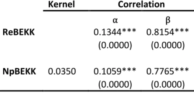
It is possible to nest an alternative and competitive parametrization, without passing through the factorization of Ž . I will refer to this model as ReBEKK.
Instead of using a DCC-GARCH type recursion, it is possible to adopt a BEKK-type framework. Without using the classical BEKK model of Baba, Engle, Kraft and Kroner (1995), I will refer to the multiplicative BEKK model of Hafner and Lindton (2010) that, through covariance targeting, introduced a first order scalar BEKK,
35
directly fitted to the series of realized variance covariance matrix, with the following form:
Ž = Ž̅ 1 − − ¡ + t + ¡Ž Where and ¡ are positive scalars and + ¡ < 1.
Moreover, since I wanted to increase comparability of my model, it was possible to add another parametrization, based on the decomposition of Ž into a long run covariance matrix and a short run component, respectively £ = $$y and Ž∗, such that:
Ž = $ Ž∗$y
In this case, $ is obtained through a Cholesky factorization of long run matrix L. The latter is estimated by the non-parametric smoother of Nadaraya-Watson, used in the estimation process for all the element of realized variance covariance matrices. For the short run component, I restored the multiplicative scalar BEKK, where, differently as in the first parametrization, I imposed the mean reversion condition in its dynamics, through /1, so that:
Ž∗ = 1 − − ¡ /1+ t∗ + ¡Ž∗
where t∗ = $ t $ y and it is a variance covariance matrix purged of its long run component.
I will refer to this model as Np-ReBEKK.
For both BEKK parametrization, the estimation process was carried out through a one-step loglikehood-based approach, previously used:
£ = 5 u¢†|Ž | + Ž t
9 :
2.4 Covariance Targeting
Before turning into the presentation of the other model used in this work, I have to discuss one another feature of the new parametrization offered by DCC-CAW-Mem, that is also at the basis of the estimation procedure of one of the BEKK parametrization of Section 2.3: the covariance targeting.
36
To understand its usefulness, consider that, even if I imposed a scalar specification of my model, the number of parameters to be estimated was proportional to the number of assets, so that the estimation became cumbersome, if a high number of assets is included in the model design. Hence, in order to exploit the advantages of working with a great number of assets with intraday data, I needed a quick and simple way to guarantee a feasible estimation in the maximum likelihood framework. For this reason, both in DCC-CAW-MEM and in BEKK parametrizations, I resorted to targeting approach, that consists in pre-estimating the constant intercept matrix in the model specification.
More specifically, in the DCC-CAW-MEM
- = Ž̅ 1 − − ¡ + t + ¡- 4 = -∗ / - -∗ /
Targeting is imposed in - structure ensures that the conditional correlation will be identical to the sample unconditional correlation of the data. This is strictly achieved by computing the sample covariance matrix of standardized residuals Ԑ that come from the n univariate MEM (1,1) estimation, so that:
Ž̅ = ª Ԑ Ԑy = 5 Ԑ Ԑ9 y :!
Moreover, also the first order scalar BEKK model is based on the covariance targeting, since its recursion has the following form:
Ž = Ž̅ 1 − − ¡ + t + ¡Ž
Where Ž̅ is the unconditional long run variance covariance matrix. In this case, targeting implies the use of a sample covariance estimator for S and the maximization of the likelihood function with respect to the parameters α and β (maximization is made conditionally on the estimates of the long run covariance)9.
37
2.5 Additional models
For the completeness of my analysis, I included one additional model for realized volatility, that combines two different specifications: the Heterogeneous Autoregressive model for the Realized Variance (HAR-RV) of Corsi (2009) and the dynamic structure of a DCC of Engle (2002).
In the original formulation of 2003, Corsi allowed for heterogeneity in the traders’ time horizons, by introducing an additive cascade of partial volatility at the different time-points: daily, weekly and monthly, even if more other component could be easily added.
Despite this model formally does not belong to the category of long memory models, Andersen, Bollerslev and Diebold (2007) and Wang, Bauwens and Hsiao (2013) have found that it provides a very good fit for most volatility series. Thus, the HAR-RV model could be considered a genuine long memory model, and in contrast to the other long memory model, it could be easily estimated through OLS procedures. Moreover, instead of considering the DCC of Engle separately from the HAR-RV, I decided to combine them, by using a two-steps estimation log-likelihood-based approach. In particular, the estimation required:
1. in step 1, a multivariate DCC model was directly run on realized kernel time series, in order to obtain the correlation coefficient among series;
2. in step 2, the standardized residuals Ԑ of DCC model were used to reconstruct the volatility series œ that constitute the inputs of the OLS model, that allowed to find the HAR parameters:
œ7 = ¡{+ ¡gœ + ¡¬œ -, + ¡Šœ , + ®7
With ® is a random error.
Finally, as baseline model, the vMEM of Cipollini et al. (2012) has been estimated, through an equation by equation estimation approach.
As for the univariate MEM model examined in the Section 2.1, the basic parametrization is the following:
38
ℎ Ԑ | ~} vv ”,1” where ⊙ is the Hadamard product and also in this case S = S , • . The random variable is defined as k∗1 vector ] | ∽ • 1, z . For the previous conditions:
4 | = S 4 | = S Sy⊙ ±
As for the univariate framework, in the multivariate context the conditional expectation is defined as:
S = – + 5 oH4 H+ 'HS H ž
H:
In my study, in order to estimate this recursive form –, o ;k ' are scalar parameters. Also in this case, during the estimation procedure, the usual constraints for positiveness and stationarity are imposed – >0, o > 0, ' > 0 and – + o + ' < 1.
2.6 Estimation Procedures Concluding Remarks
All the parametric models have been estimated through a maximum likelihood-based approach: excluding the HAR-DCC model and the vMEM, the estimation is done by a unique likelihood function, based on the Wishart distribution made on the series of realized variance covariance matrices Ct.
The log-likelihood function has been defined as: −T2 5 u¢†|Ž | + Ž t
9 :
and, as it was shown, it is very general, in the sense that it can be used, in case of absence of microstructure noise, whatever will be the formulation for volatility and correlation dynamics. For those models, I decided to use a one-step approach in order to simplify the inference and to easily compute standard error s and model selection criteria. Moreover, in the case of non-parametric formulation, as for Np-ReBEKK model, the estimation requires two steps: the computation of the kernel smoother for accounting the long run co-movements in variance covariance matrices, and then the short run component is estimated through the previously defined ML approach. In
39
addition, the HAR-DCC model is the only one model that has been estimated through a two steps procedure, by firstly estimating the DCC parameters, followed by the estimation of HAR coefficient, through the standardized residuals. Finally, the vMEM has been estimated by an equation by equation approach, even if, instead of using a GMM estimator suggested by Cipollini (2012), I followed a ML approach, by adapting the univariate estimation procedure of Brownlees et al (2011).
40
Chapter 3
Evidence from Real Data
Abstract:
This chapter presents the empirical analysis conducted on a twenty realized kernel financial time series, and the corresponding daily series of realized variance covariance matrices.
Firstly, I will present the dataset being used and the cleaning procedures adopted to obtain it. Then, after providing the full sample estimation results by comparing the models in term of information criteria, I finally presented the theoretically framework for financial one-step ahead forecasts and their comparisons.
41
3.1 Dataset
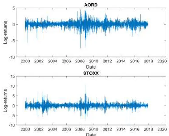
In carrying out my empirical analysis, I considered a dataset of annualized realized kernel of volatility for twenty (20) financial indices, provided by the Oxford Man Institute10, from January 3, 2000 to December 5, 2017.
As stated by Bandorff, Nielsen, Hense, Lunde and Sheppard (2002), realized kernel is a consistent estimator of realized volatility, and it is also robust respect to microstructure noise of the markets.
The included stocks are: AEX Index, All Ordinaries , BVSP BOVESPA Index , Down Jones Index , CAC 40 , FTSE 100 , FTSE MIB , FSTE STRAIT TIME Index, DAX, Hang Seng Index , IBEX 35, Nasdaq 100, Korea Composite Stock Price Index, IPC Mexico, Nikkei 225, NIFTY 50, Russel 2000, SP 500 Index, Swiss Stock Market Index and EUROSTOXX 50.
The original database contained 21 assets, but from a preliminarily analysis, it resulted that the percentage of missing values ranged between 2.45% of CAC40 and 16,78% of S&P/TSX Composite index (GSPTSE).
Moreover, from a more careful examination, it has been possible to note that for GSPTSE index, there were two years of missing values (the series starts on May 02,2002), so that I decided to drop it from the dataset. Furthermore, since I relied on standard measures and not on heavy data, in order to get a complete dataset, I deleted overnight returns (favoring the estimation accuracy). Then I choose, as treatment of missing values, a linear interpolation11 and, as a special case, in presence of a missing value at the first observation, I replaced it using the forward value.12
Additionally, for the estimation process, I had to preliminarily compute the series of realized variance covariance matrices.The daily realized covariance matrices have been computed using the CholCov estimator presented in Section 1.3.8
For a simpler read of the results, the following table reports abbreviations and the full name of the assets included in the study.
10 The database used in this thesis refers to the 0.2 version, that was retired and now at the following link https://realized.oxford-man.ox.ac.uk/data/download it’s possible to download a more recent and bigger (31 assets) library, that rely on a different cleaning and econometric procedures.
11 See Lu, Z. & Hui, Y.V. Ann Inst Stat Math (2003) 55: 197. https://doi.org/10.1007/BF02530494 12 No additive cleaning procedures are used.
42
Table 1: Data symbols. The table shows the list of symbols (column 1) used to
identify the corresponding financial time series indices (column 2).
Given the framework of analysis presented in the previous chapter, the aim of this empirical analysis is to evaluate both the in-sample and the out-of- sample performance of the models presented before.
Just for a reminder, we report a list of all the models presented in the previous sections.
Model N. parameters Parametric Semiparametric
1) vMEM (4*n) ✓ 2) DCC-CAW-MEM (4*n)+2 ✓ 3) ReBEKK [n(n+1)/2]+2 ✓ 4) Np-ReBEKK 3 ✓ 5) HAR-DCC (4*n)+2 ✓
Table 2: List of analyzed models. This table lists the estimated models with each own
number of parameters, as well as the specific parametrization.
Symbol Asset Name
AEX AEX Index AORD All Ordinaries
BVSP BVSP BOVESPA Index DJI Down Jones Index FCHI CAC 40 FTSE FTSE 100 FTSEMIB FTSE MIB
FTSTI FSTE STRAIT TIME Index GDAXI DAX
HSI Hang Seng Index IBEX IBEX 35 IXIC Nasdaq 100
KS11 Korea Composite Stock Price Index (KOSPI) MXX IPC Mexico
N225 Nikkei 225 NSEI NIFTY 50
RUT Russel 2000 SPX SP 500 Index SSMI Swiss Stock Market Index STOXX EUROSTOXX 50
43
Preliminarily I will report the results of the full sample estimation and, afterward, I will focus on the one step ahead out of sample forecasts. For the latter, the full dataset, from January 3, 2000 to December 5, 2017 is divided into two different periods:
Period I is the in-sample set for t=1, …, 4161. It corresponds to the period January 03, 2000 to December 04, 2015;
Period II is the out of sample set for the remaining 522 observations in the dataset, from December 05, 2015 to December 05, 2017, that represents the last observation included in the sample.
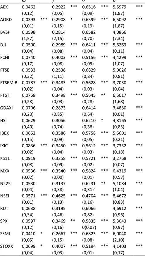
Before presenting the full sample results, I will summarize the descriptive statistics for all the time series, distinguishing the full sample, the in sample and the out of sample sets of analysis. On the basis of the kurtosis, it is possible to note that time series properly exhibit fat-tail properties and there is also a departure from the Gaussian distribution, since the skewness is different from 0 and there is positive excess kurtosis.