Fatigue assessment by energy approach during tensile tests on AISI 304 steel

(1)

A. Risitano et alii, Frattura ed Integrità Strutturale, 39 (2017) 202-215; DOI: 10.3221/IGF-ESIS.39.20

202

Fatigue assessment by energy approach during tensile

tests on AISI 304 steel

A. Risitano

C.R.P.S. srl arisitan@gmail.com

D. Corallo

University of Catania, Department of Industrial Engineering dcorallo@dii.unict.it

E. Guglielmino, G. Risitano

University of Messina, Department of Engineering

giacomo.risitano@unime.it, http://orcid.org/0000-0002-0506-8720 eguglie@unime.it, http://orcid.org/0000-0001-7793-7406

L. Scappaticci

Guglielmo Marconi University l.scappaticci@unimarconi.it

ABSTRACT. Estimation of the fatigue limit for steel ductile materials using non-destructive methods is a topic of great interest to researchers today. In recent years, the method adopted has implemented infrared sensors to detect the surface temperature and correlate it with the fatigue limit.

In previous paper, a new energy approach was proposed to investigate the fatigue limit during tensile test. The numerical procedure proposed by Chrysochoos is adopted to clean infrared images and applied to analyse the surface heat sources during tensile test. AISI 304 specimens with rectangular cross-sections are tested.

Moreover fatigue tests at increasing loads were carried out on steel by a stepwise succession, applied to the same specimen, for applying the thermographic method. The predictions of the fatigue limit, obtained by the analysis of the energy evolution during the static tests, were compared with the predictions obtained applying the thermographic method during fatigue tests.

KEYWORDS. Fatigue Limit; Mono Axial Static Test; Thermographic Method.

Citation: Risitano, A., Corallo, D.,

Guglielmino, E., Risitano, G., Scappaticci, L., Fatigue assessment by energy approach during tensile tests on AISI 304 steel, Frattura ed Integrità Strutturale, 39 (2017) 202-215.

Received: 10.06.2016 Accepted: 10.10.2016 Published: 01.01.2017

article under the terms of the CC-BY 4.0, which permits unrestricted use, distribution, and reproduction in any medium, provided the original author and source are credited.

(2)

203

INTRODUCTION

n the last thirty years, the methodologies adopted to estimate conventional fatigue limit for steel ductile materials has implemented with infrared sensors. Indeed, the surface temperature of the specimen has been correlated to stress applied during the fatigue test. In 1986 [1], Curti et al. were the first researchers that developed and used thermography to explore the thermal map over the surface of a specimen and thereby determine the fatigue limit. In 1988 [2], Luong illustrated three advantages of infrared thermography technique: observation of the physical processes of damage and failure in metals; detection of the occurrence of intrinsic dissipation; evaluation of the fatigue strength in a very short time. In 2000 [3], La Rosa et al. presented a new methodology (Risitano Method) for the determination of the conventional fatigue limit of materials or mechanical components. In 2002 [4], Fargione et al. presented a procedure for the definition of the whole fatigue curve by the thermographic method. In 2005 [5], Curà et al. presented a new thermographic method based on an iteration procedure for the determination of the fatigue limit of materials and components. The thermographic results have been compared to the corresponding obtained by means of a different thermographic method [3]. In 2007 [6], local 1D and 2D expressions of the heat diffusion equation were used to

separately estimate the coupling and dissipative sources accompanying the fatigue testof an aluminium alloy. In 2007 [7],

Meneghetti defined a theoretical model in order to derive the specific heat loss per cycle from temperature measurements performed during the fatigue test. In 2008 [8], Crupi developed a theoretical model, introducing new relationships able to correlate the damping with other mechanical properties defining the different failure modes. In 2010 [9], Amiri et al. showed that the slope of the temperature plotted as a function of time at the beginning of the test can be effectively utilized as an index for fatigue life prediction. In 2013 [10], Fargione et al. applied thermographic method on mechanical components to individuate crack paths and damage evaluation. In 2014 [11], Crupi et al. were the first researchers that detected the radiometric surface temperature during ultrasonic fatigue tests in order to extend the thermographic method in very high cycle fatigue regime.

Chrysochoos et al. in [12] have determined experimentally the energy balances of pseudo-elastic behaviour of a shape memory alloy using IR techniques and in [13], using infrared image processing, have determined the evolution of the heat source’s distribution on steel samples during monotone tension tests. The same authors in [14] presented an infrared data processing developed to analyse the calorific manifestations accompanying elastoplastic transformation during tensile tests. And in [15] have investigated experimentally on thermal and calorimetric effects induced by Luders band propagation during monotonic and quasi-static tensile tests.

In previous papers, authors investigated the variation of temperature during static tensile tests of plastic [16] and metallic [17] materials to connect the variation of the slope of the stress strain versus temperature curve with the conventional fatigue limit of the material. In [18], authors suggested that during quasi-static tensile tests the area, where first irreversible plasticization occurred, is detectable on T vs curve by the variation of temperature (slope). This variation identifies the transition zone between thermoelastic and thermoplastic behaviour, or in other words, the beginning of irreversible micro-plasticisation.

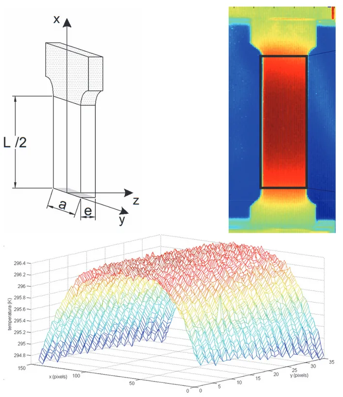
Figure 1:Specimen dimensions [mm].

The method proposed in this paper is based on hypothesis that high cycle fatigue failures occur when local stresses generate irreversible plastic deformation amplified by micro-defects. For some static tensile test parameters, such as load speed [N/s], the change of the slope is not easy to define; in these cases the evaluation of the dissipation energy can help

(3)

204

evaluation of transition zone. In the present paper, a new approach is proposed to investigate the fatigue limit during tensile static tests. Particularly, a numerical approach to estimate specific energy is developed, based on the method proposed by Chrysochoos and Louche [14, 15, 19]. Therefore, the authors estimated the dissipation and the area where the first increase of energy occurs. The macro average stress value applied (load/area) on the specimen, when the first increase of temperature occurs, corresponds to conventional fatigue limit of material.

In this paper a qualitative method, to improving an already proposed approach of the authors by using a different energetic parameter instead of the temperature is here presented. AISI 304 specimens with rectangular cross-sections were tested using static test and fatigue tests (R= -1). During static tensile and fatigue tensile tests, IR camera has been used to evaluate energy dissipations. In addition, the fatigue limit was determined using thermographic method and results have been compared to static results.

MATERIAL AND METHODS

he tests were performed in two phases. In the first phase, the energy dissipation of the specimens was evaluated during tensile static test by a IR camera. In the second phase, the conventional fatigue limit was found during fatigue tests by thermographic method [1,3, 4]. The results of the two phases were compared.

The material was AISI 304 steel; eight specimens were produced. Fig. 1 illustrates the shape and dimensions of the specimen. Four specimens were used for the static tensile tests and four were used for the fatigue tests employing thermographic method. All the specimens are black painted and their thermal emission coefficient was 0,92±5. A Zwick Z100 universal tester was used for the static tensile tests. During the static tests, the surface of the specimen was monitored using a FLIR_SC 3000 infrared camera. The tests were performed at a crosshead speed of 3 mm/min; the

average nominal strain was ~9.0910-4_s-1_{(calculated by speed test/gage length): physical transformation can be considered}

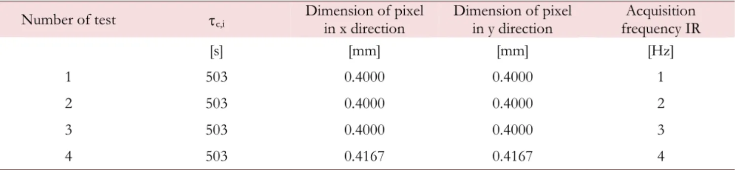
quasi-static. In Tab. 1, the material characteristics are reported. In Tab. 2, time constant and spatial resolution for the first phase of the tests are reported.

In the second phase, the fatigue tests were performed using an INSTRON 8872 test machine and surface temperature was recorded during the test using an infrared machine FLIR-SC 3000 (the acquisition frequency of the IR image was 0.2 Hz). For the second phase, the load ratio was R= -1 and the test fatigue frequency was 5 Hz.

density thermal conductivity specific heat coefficient of thermal _expansion yield stress

[kg/m3_{] [W/mK] [J/kgK] [1/K·10}-6_{] [MPa]}

7900 15 502.4 17 325

Table 1:Thermomechanical properties of AISI 304.

Number of test c,i Dimension of pixel _{in x direction} Dimension of pixel _{in y direction} _{frequency IR}Acquisition

[s] [mm] [mm] [Hz]

1 503 0.4000 0.4000 1

2 503 0.4000 0.4000 2

3 503 0.4000 0.4000 3

4 503 0.4167 0.4167 4

Table 2:Time constant and spatial resolution for the four tensile static tests.

THEORY AND CALCULATION

o simplify the theoretical approach, according Chrysochoos and Louche [14, 15, 19], the following hypotheses were used in analysing the heat released during the static tensile tests:

1. A quasi-static physical transformation during the static test occurs; thus permitting the use of classic rules

T

(4)

205

for the internal variables.

2. The specific heat C(for the constants  and ) is assumed to be independent respect to the internal state of the

material and hardening.

3. The conduction is linear isotropic, and thus, the Fourier law q   is valid. k 

4. The total derivatives with respect to time are reducible at partial derivatives; therefore, it is possible to neglect the

convective terms, and the transformation velocities can be considered negligible.

5. The external temperature  is assumed to be time/space constant; therefore, the external flux re is considered to

be independent of time.

6. The initial temperature (x,y,z,0) of any point can be considered to be coincident with the external temperature



To understand the logical process, we have to start following points presented in [20], where Maugin connected the mathematical theory of plasticity and fracture to the field of thermomechanical for metallic material. Starting from the second law of thermodynamics and the principle of continuity of mass, the inequality equation of Clausius-Duhem can be written as follows:

r t

int 0

   

Intrinsic and thermal dissipation are respectively:

v e p r t A q int : :                       

where



 v :e  :p



is the inelastic component and



A 



is the hardening dissipation that the material uses to determine its own internal characteristics.

By the theorem of energy in the local form e:D r  _e q, using the previous assumptions and the temporal

derivatives of the Helmholtz’s potential (), it is possible write the following equation of heat diffusion:

e r _e e C_{ }_, k 2 _int : : r                          _

Assuming that the coupling terms between temperature and internal variables is negligible  : 0  

 _

  , the diffusion

equation can be write:

sm e C , k 2 r      _with e sm intr _e :             (1) where:

   



  , ,



is the Helmholtz free energy;  re is the external heat flux;

 int r is the intrinsic dissipation per unit of volume of irreversible phenomena;

 is the internal temperature;

 smincludes all terms that yield internal dissipations and is called the thermoelastic or isentropic term.

Focusing the attention on the first part of static tensile test, it is possible to individuate the thermoelastic zone where transformations are reversible. Focusing on the first part of the true curve while maintaining a constant external temperature during testing, visco-plastic phenomena can be neglected, and it is possible to set all the terms of intrinsic

(5)

206

dissipation to zero



_int_r 0



.Consequently, the volumetric density of the heat sources of a mechanical nature sm can

be written as the following: e sm 0 _e :           (2)

The only term that describes the dissipative process is the thermoelastic coupling. This equation is easily resolvable when considering an isotropic and homogeneous material for which      e,  e, 0. Indeed, assuming the previous positions, the Helmholtz free energy becomes:



 ,



₀

 

 K



   ,



Tr

 

 2 Tr

 

2

      (3)

where:

 0() is the initial free energy when the material is unstrained;

  is the temperature variation in comparison with the reference temperature 0;

  and  are the Lamé coefficients;  K is the bulk modulus;

  is the thermal dilatation coefficient.

Using Eq. (3) and Schwarz’s theorem, it is possible to write the Duhamel-Neumann equation calculating the derivate of

    with respect to  e:





 



K , Tr



I 2           _{  } _{ } _  (4)

where by, the derivative with respect to  can be written







K ,



I K



,



I  _ _{  } _{  }    _{ }  _ _   (5)

Assuming the application of this equation to the transformation for which the elastic property and the thermal dilatation coefficient are temperature independent, Eq. (2) can be written as the following:





 

e e e e e sm _e : 0  : K 0I: K , 0 Tr                       _ _        (6)

Analysing Eq. (6), it is possible to note that during a tensile test (strain is positive) all the coefficients are positive; therefore the equation will yield a negative result. This result implies that the material absorbs heat from the outside for elastic deformation and previous hypothesis. In this phase, the behaviour of the material is perfectly thermo-elastic and

the temperature of the specimen decreases. Performing the test at a constant strain rate, the quantity sm will be constant

(the coefficients are considered to be independent of the stress state). When local plasticisation occurs, the positive heat

sources are activated



_int_r 0



, causing a consequent increasing in temperature.

The next step is to solve the previous expression. Assuming the following geometry of the specimen as the integration domain {L, a, e}, it is possible to write Eq. (1) using average values:

c i T C _, T T s ,                   ₍₇₎

(6)

A. Risitano et alii, Frattura ed Integrità Strutturale, 39 (2017) 202-215; DOI: 10.3221/IGF-ESIS.39.20 207 with









e T x y t x y z t dz e₀ 1 , , 



 , , , and





e s x y t dz e₀ 1 , , 



 where:

  is the thermic diffusivity;

 c,i is the time constant for the heat dissipation by convection and radiation on the faces z= 0 and z= e;

 and is the material density.

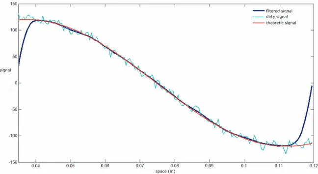
A Matlab® code was developed to evaluate the dissipative process using an approach proposed by Chrysochoos et al. [14, 15, 19] and specified in the introduction. A series of IR images of an unstressed specimen were recorded to remove the

signal arising from external noise. A low-pass filter based on a normalised Gaussian curve was built to ensure that the

spectrum frequency of the signal does not change (Fig. 2).

Figure 2:Example of processed signal.

RESULTS AND DISCUSSION

Static Tensile Tests

uring static tests of common engineering metals, the temperature evolution on the specimen surface, detected by means of an infrared camera, is characterized by three phases: an initial approximately linear decrease due to the thermoelastic effect (phase 1), then the temperature deviates from linearity until a minimum (phase 2) and a very high further temperature increment until the failure (phase 3). The first deviation from linearity, which corresponds to the end of the phase 1, was correlated to the fatigue limit [18].

Focusing on elastic part of the stress-strain curves, Eq. (5) was applied to infrared images. The domain of analysis was identified (Fig. 3) and thermal signal was filtered in space and time. The temperature and dissipation trends were obtained for each specimen tested. Fig. 4 shows the results of a static tensile test.

The specimens were coated with black paint and the surface temperature of the specimen was monitored during the whole tensile test with an infrared camera (FLIR_SC 3000). The behaviour of temperature and heat sources were investigated during tensile static test. The area where the first energy dissipation occurs were identified. The spatial identification has been made considering the area "hottest" of the specimen. The temporal identification was made by considering the slop present in the curves Dissipation vs. Time and Temperature vs. Time.

After processing the infrared images, the average thermal and dissipative evolution on a subdomain of the section of the specimen were plotted (Fig. 5).

(7)

208

Figure 3:IR domain.

From the N x M area (N: number of columns; M: number of lines) for all tests, square subdomains defined by 4 x 4 pixels were selected and were separated from each other by 5 pixels; during the extrapolation phase a set of points was used

rather than a single pixel. As mentioned above, the average strain speed was ~9.1104_s-1_{and being the spatial resolution of}

0.4, the pixel's displacements were negligible.

(8)

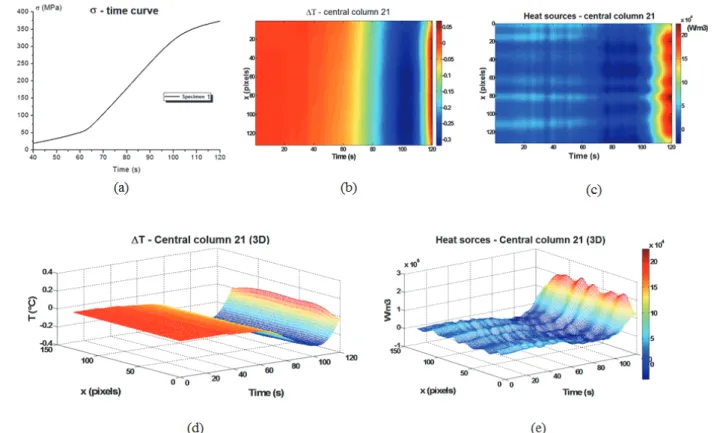
209 Figure4: Load vs. Time curve (a), Waste Heat 2D Map vs. Time (b), Dissipative Energy 2D Map vs. Time (c), Waste Heat 3D Map vs. Time (d), Dissipative Energy 2D Map vs. Time (e).

Figure 5:Plot subdomains.

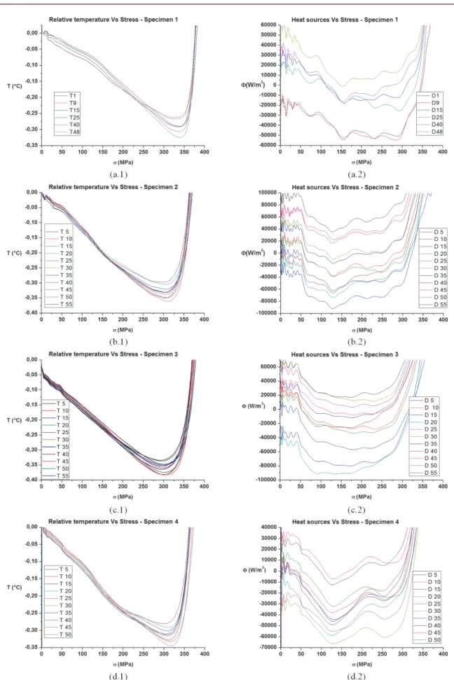
According to Eq. (7), trends of temperature and stress were plotted as a function of time (Fig. 6). As shown in some papers, for example in [18], the conventional fatigue limit could be estimated: the macro-stress value at which the linear trend ends is the conventional fatigue limit. However, evaluating the linearity temperature change may not be easy, as in the present case [21]. Indeed, as show in Figs. 6.a2, 6.b2, 6.c2 and 6.d2 the slope of the temperature curves is not easy to capture. In that case, the analysis of heat sources curves can help much (Fig. 6.a3, 6.b3, 6.c3 and 6.d3). Similarly to the temperature, it is possible to define the conventional fatigue limit as the macro average applied stress value (load/area) where dissipative energy trend has a changes. Figs. 6 and 7 clarify how the dissipative curves are able to define the end of the elastic phase (e.g. Fig. 6.a3).

For each specimen tested, macro average applied stress value corresponding to the change of dissipation trend was estimated. All values are reported in Tab. 3. The average of the fatigue limit was 134.0 MPa and standard deviation was 10.95 MPa.

Specimen 1 Specimen 2 Specimen 3 Specimen 4

0 [MPa] 150 128 132 126

(9)

210

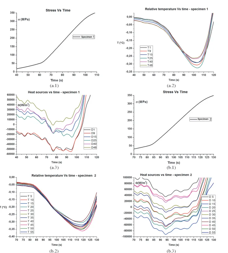
Figure 6:Tensile Stress vs. Time curve (1), Temperature vs Time curves (2) and Dissipative Energy vs Time curves (3) during tensile static tests for all specimens (a, b, c and d) are reported (continue).

(10)

211 Figure 6:Tensile Stress vs. Time curve (1), Temperature vs Time curves (2) and Dissipative Energy vs Time curves (3) during tensile static tests for all specimens (a, b, c and d) are reported.

(11)

212

Figure 7:Temperature (1) and heat sources (2) as a function of nominal stress during tensile static tests for all specimens (a, b, c and d) are reported.

(12)

213

Fatigue Tests

The specimens, investigated under fatigue loading, have the same geometry of those used for the static tests and are made from the same steel and servo-hydraulic load machine (INSTRON 8872) was used. Fatigue tests were carried out at R = 0.1 and f = 5 Hz, applying increasing loads by a stepwise succession (applied to the same specimen), starting from 33 MPa with steps of 33 MPa every 1.000 cycles. In order to apply the thermographic method, the specimens were coated with black paint and the surface temperature of the specimen was monitored during the whole fatigue test with an infrared camera

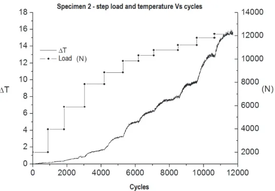
Fatigue tests were performed according to the classical thermographic method [4] to validate the results of the static tests. For each specimen, many steps were used to increase the load. Each load step is considered completed when the temperature detected by the IR sensor at the most stressed point (at a higher temperature) is stabilised. After temperature stabilisation, the test follows, immediately imposing a further step to a greater load and waiting again until stabilisation before proceeding to the next step [3] (Fig. 8).

Figure 8:Experimental data for specimen No. 2 during fatigue test.

All values are reported in Tab. 4. The average fatigue limit was 119.3 MPa standard deviation was 6.24 MPa. The conventional fatigue limit is similar to the value estimated by the tensile test. In fact, the deviations that exists between the two values is ~11%, the typical deviations of classical experimental test. This value is in according with the value presented in literature for similar machined AISI 304 steel: e.g. ~125 MPa [22].

Specimen 1 Specimen 2 Specimen 3 Specimen 4

0 [MPa] 115 123 113 126

Table 4:Estimated conventional fatigue limits by TM fatigue tests.

CONCLUSIONS

n this paper, a procedure to evaluate the energy released as heat for local micro-plasticisation was applied to evaluate the end of the elastic phase in static tensile tests. This procedure permits to estimate the fatigue limit using simple static tests when the temperature evolution is not easy to define [21]. Particularly, the authors used the Chrysochoos indications [14, 15, 19] to implement a qualitative method to evaluate the changing trend in the Dissipated Energy vs. Time curve on the specimen surface during static tensile tests. The results indicated that the changing trend in Dissipated

(13)

214

Energy vs. Time curve is more prominent than the changing slope in the Temperature vs. Time curve for the estimation of the stress at which the complete linear elastic phase ends.

The method was applied to AISI 304 steel. The fatigue limit determined by the static tensile test was compared with the value determined by fatigue tests for equivalent specimens loaded with a load ratio R= -1. The values of the average conventional fatigue limit for the two adopted methods (the static test and fatigue test) were relatively close (134.0 MPa versus 119.3 MPa), within normal fatigue test dispersions (~11%,) and in according with value presented in literature (~125 MPa).

REFERENCES

[1] Curti, G., La Rosa, G. Orlando, M., Risitano, A., Analisi Tramite Infrarosso Termico della Temperatura Limite in Prove di Fatica, XIV AIAS Italian National Conference, Catania, (1986).

[2] Luong, M.P., Fatigue limit evaluation of metals using an infrared thermographic technique, Mech. Mater., 28 (1988) 155–163.

[3] La Rosa, G., Risitano, A., Thermographic methodology for the rapid determination of the fatigue limit of materials and mechanical components, Int. J. Fatigue, 22 (2000) 65–73.

[4] Fargione, G., Geraci, A., La Rosa, G., Risitano, A., Rapid Determination of the Fatigue Curve by the Thermographic Method, Int. J. Fatigue, 24 (2002) 11–19.

[5] Curà, F., Curti, G., Sesana, R., A new iteration method for the thermographic determination of fatigue limit in steels, Int. J. Fatigue, 27 (2005) 453–459.

[6] Morabito, A.E., Chrysochoos, A., Dattoma, V., Galietti, U., Analysis of heat sources accompanying the fatigue of 2024 T3 aluminium alloys, Int. J. Fatigue, 29 (2007) 977–984.

[7] Meneghetti, G., Analysis of the fatigue strength of a stainless steel based on the energy dissipation, Int. J. Fatigue, 29 (2007) 81-94.

[8] Crupi, V., An Unifying Approach to assess the structural strength, Int. J. Fatigue, 30 (2008) 1150–1159.

[9] Amiri, M., Khonsari, M.M., Rapid determination of fatigue failure based on temperature evolution: Fully reversed bending load, Int. J. Fatigue, 32 (2009) 382–389.

[10] Fargione, G., Tringale, D., Guglielmino, E., Risitano, G., Fatigue characterization of mechanical components in service, Frat. Integ. Strutt., 26 (2013) 143-155.

[11] Crupi, V., Epasto, G., Guglielmino, E., Risitano, G., Investigation of very high cycle fatigue by thermographyc method, Frat. Integ. Strutt., 30 (2014) 569-577.

[12] Chrysochoos, A., Pham, H., Maisonneuve, O., Energy balance of thermoelastic martensite transformation under stress, Nucl. Eng. Des., 162 (1996) 1-12.

[13] Chrysochoos, A., Louche, H., Analyse thermographique des mèanismes de localization dans des aciers doux, C. R. Acad. Sci. Paris, 326 Série II b (1998) 345-352.

[14] Chrysochoos, A., Louche, H., An Infrared Image Processing to Analyse the Calorific Effects Accompanying Strain Localization, Int. J. Eng. Sci., 38 (2000) 1759-1788.

[15] Louche, H., Chrysochoos, A., Thermal and Dissipative Effects Accompanying Lüders Band Propagation, Mater. Sci. Eng. A –Struct., 307 (2001) 15–22.

[16] Risitano, A., La Rosa, G., Fargione, G., Clienti, C., Risitano, G., A First Approach to the Analysis of Fatigue Parameters by Thermal Variations in Static Tests on Plastics, Eng. Fract. Mech., 11 (2010) 2158–2167.

[17] Risitano, A., Clienti, C., Risitano, G., Determination of Fatigue Limit by Mono-Axial Tensile Specimens Using Thermal Analysis, Key Eng. Mat., 452-453 (2011) 361-364.

[18] Risitano, A., Risitano, G., Determining Fatigue Limits with Thermal Analysis of Static Traction Tests, Fatigue Fract. Eng. M., 36 (2013) 631-639.

[19] Chrysochoos, A., Infrared Thermography, a Potential Tool for Analysing the Material Behaviour, Mec. Ind., 3 (2002) 3–14.

[20] Mougin, G.A., The Thermomechanics of Plasticity and Fracture, Cambridge University Press, Cambrige, (1992). [21] Corigliano, P., Crupi, V., Epasto, G., Guglielmino, E., Risitano, G., Fatigue Assessment by Thermal Analysis during

Tensile Tests on Steel, Procedia Engineering, 109 (2015) 210-218. DOI: 10.1016/j.proeng.2015.06.215

[22] Di Schino, A., Kenny, J.M., Grain size dependence of the fatigue behaviour of a ultrafine-grained AISI 304 stainless steel, Materials Letters, 57 (2003) 3182–3185.

(14)

215

NOMENCLATURE