A coopetitive-dynamical game model for currency markets stabilization

AAPP | Atti della Accademia Peloritana dei Pericolanti

Classe di Scienze Fisiche, Matematiche e Naturali

A COOPETITIVE-DYNAMICAL GAME MODEL FOR CURRENCY MARKETS STABILIZATION

DAVIDCARFÌa∗ANDFRANCESCOMUSOLINOb

ABSTRACT. The aim of this paper is to propose a dynamical methodology to stabilize the currency markets and at same time to address, indirectly, the Credit Crunch phenomenon. We adopt Game Theory and, specifically, the new mathematical model of Coopetitive Game proposed in literature by D. Carfì with some its associated dynamical aspects. Our idea is to save the Euro (or other currencies) from speculative attacks, by introducing a currency transactions tax. Specifically, we focus on a real economic operator - our first player - and on an investment bank - our second player. The unique solution that allows both players to gain something, and therefore the only one collectively desirable, is represented by an agreement, between the two subjects, on the division of the maximum collective gain. Finally, we propose also a possible division of gains (even more advantageous than the previous one) in a coopetitive context, where the two above economic subjects use a loan by the European Central Bank (ECB), to obtain a greater gain.

1. Introduction

1.1. Speculators and financial markets: a possible solution. The recent financial crisis has shown that, in order to stabilize markets, it is not enough to prohibit or to restrict short-selling. In fact, big speculators can influence the financial market and take huge advantage from arbitrage opportunities, caused by themselves.

In this paper, by the introduction of a tax on currency transactions, we propose a method aiming to limit the speculations of medium and big financial operators and, consequently, a way to make more stable the Euro markets.

Moreover, our aim is attained without inhibiting the possibilities of profits. At this purpose, we will present and study a natural and quite general normal form game - as a possible standard model of fair interaction between two financial operators - which gives to both players mutual economic advantages. Finally, we shall propose an even more advantageous coopetitive model and one its possible compromise solution.

1.2. Literature review. In this paper, we shall refer to a wide variety of literature. First of all, we shall consider some papers on the complete study of differentiable games and related mathematical backgrounds, introduced and applied to economic theories since 2008 by Carfì (see Baglieri, Carfì, and Dagnino2010; Carfì2008a,b,2009a,b,c,d,e,2010a,b,2011; Carfì and Cvetko-Vah2011; Carfì, Magaudda, and Schilirò2010; Carfì and Ricciardello 2009,2010).

Specific applications of the previous methodologies, also strictly related to the present model, have been illustrated by Carfì and Musolino (2011a,b,2012a,b,2013a,b,c,2014, 2015a,b) and Musolino (2012). Other important applications of the complete examination methodology were introduced by Carfì and coauthors (Agreste, Carfì, and Ricciardello 2012; Arthanari, Carfì, and Musolino2015; Baglieri, Carfì, and Dagnino2012,2015; Carfì 2012; Carfì and Fici2012; Carfì, Gambarelli, and Uristani2013; Carfì and Lanzafame2014; Carfì et al.2012,2013; Carfì, Patanè, and Pellegrino2011; Carfì and Perrone2011a,b,c, 2012,2013; Carfì and Pintaudi2012; Carfì and Ricciardello2012,2013a,b; Carfì and Schilirò 2011a,b,c,2012a,b,c,d,2013, 2014; Carfì and Trunfio2011; Okura and Carfì 2014).

In this paper, moreover, we shall use sistematically some researches of economic liter-ature (Anonymous2012; Asch1952; Deutsch and Gerard1955; Ford, Kelsey, and Pang 2013; Hull2002; Mediobanca2012; Milgram1964; Onaldo2012; Palley1999; Scharfstein and Stein1990; Wei and Kim1999; Westerhoff and Dieci2006).

1.3. Euro-Dollar market. For nearly eight years from Jenuary 2001, Euro has had a upward trend versus the U.S. Dollar and in April 2008 Euro peaked out at 1.6 a U. S. Dollar. But, after this date, Euro has declined by 17%, until March 2012 as shown in Fig. 1 (see Anonymous2012).

FIGURE1. U.S. Dollar-Euro exchange rate.

1.4. First player in our model. As our first player we choose an exemplary Multinational Enterprise (MEME) with a huge turnover and often exposed to currency risk. But the ordinary activities of a multinational enterprise is not, usually, to act on the currency market paying attention to the fluctuations of the currency values. So, very often, multinationals spend pharaonic sums for the conclusion of derivative contracts for hedging against currency risk.

1.5. Second player in our model. As our second player we choose an exemplary Bank that acts constantly on the financial markets.

1.6. Credit crunch in the Euro-area and ECB. Our model could also address indirectly the problem of credit crunch. In fact, in the last years, despite the banking world has available a huge amount of money (on Dec. ’11 and on Feb. ’12 the ECB loaned money to banks at the rate of 1%, respectively 490 and 530 billion Euros), there is no available money in the real economy. This phenomenon has begun to show its first sign of life from the second half of ’08, and it reached its peak in Dec. ’11.

The credit crunch is a wide phenomenon: Europe shows a decrease of 1.6% in loans to households and businesses. In Italy, this phenomenon is particularly pronounced, because the decline in loans was even of 5.1% from 2008.

Where’s the money loaded by ECB?Badly, the money remained caged in the world of finance:

• with some of the money from ECB, banks bought government bonds, so the spread went down (Fig. 2) (see also Onaldo2012);

• another part of the money is used by the banks to rectify their assets in accordance with EBA requirements (European Banking Authority);

• the rest of the money was deposited at ECB, at the rate of 0.5% (lower than the rate at which they received it).

Moreover, from the second half of ’08, the deposits of European banks at ECB are quadrupled.

FIGURE2. The 10-years government bonds trend of main European States

1.7. Final tasks of our model. In view of this, our model takes a different dimension and different expectations:

a: Bank puts money in the real economy, by lending to ME;

b: ME, even if it does not use the money directly in the real economy, could adopt the gains for its business activities or for a possible increase of employment; c: the bank eliminates the risk of losing money because of the economic crisis and it

obtains a gain, by a “fair" agreement with ME (which gains something too); d: the credit crunch, by our model, could be gradually attenuated, and might,

eventu-ally, disappear;

e: finally, the above positive effects will appear magnified by the intervention of ECB, by adopting a coopetitive strategic interaction.

2. Financial preliminaries

Here, we recall the financial concepts that we shall use in the present article.

(1) Any (positive) real number is a (proper) purchasing strategy; a negative real number is a selling strategy

(2) The spot market is the market where it is possible to buy and sell at current prices. (3) Futures are contracts which imposes to the contractors the exchange, for a price agreed at the sign of contract, a specified quantity of the underlying commodity, at the expiry of the contract.

(4) In derivatives market there are three main categories of operators, depending on the purpose with which use the derivative contract: hedgers, speculators and arbitrageurs (Hull2002).

• Hedgers use forwards and futures to reduce the risks resulting from their exposures to market variables. Forward hedges eliminate the uncertainty on the price to pay for the purchase (or receivable for the sale) of the underlying asset, but not necessarily lead to a better result. The use of the derivative allows to neutralize the adverse trend of the market, offsetting losses/gains on the price of the underlying asset with the gains/losses obtained on the derivatives market.

• Speculators realize investment strategies, buying (or selling) futures and then sell (or buy) them at a price higher (or lower). Who decides to speculate assumes a risk about the favorable or unfavorable trend of the futures market. The futures market offers a financial leverage to speculators, which are able to take relatively large positions with a low initial outlay.

• Arbitrageurs take the offsetting positions of two or more contracts to lock in a risk-free profit, and take advantage of a price difference between two or more markets. The arbitrageurs exploit a temporary mismatch between the performance (intended to coincide when the contract expires) of the futures market and the underlying market.

(5) A hedging operation through futures consists in purchase of futures contracts, in order to reduce exposure to specific risks on market variables (in this case on the price). In practice, the loss potential that is obtained on the spot market (the market at current prices) was offset by the gain on futures contracts.

(6) A hedging operation is said perfect when it completely eliminates the risk of the case.

(7) The futures price is linked to the underlying spot price. We assume that: • the underlying commodity does not offer dividends;

• the underlying commodity hasn’t storage costs and has not convenience yield to take physical possession of the goods rather than futures contract;

• the general relationship linking the futures price F, with delivery time T , and spot price S0, with interest capitalization at the time T , is F = S0uT, where u= 1 + i is the capitalization factor of the futures and i the corresponding unit interest rate (by i we mean the risk-free interest rate charged by banks, the so-called LIBOR rate). If not, the arbitrageurs would act on the market until futures and spot prices return to levels indicated by the above relation.

3. The game and stabilizing proposal

3.1. The description of the game. The strategic game G, we propose for modeling our financial interaction, requires a construction on 3 times, say time 0, 1 and 2.

(1) At time 0:

• ME knows the quantity of his U.S. Dollar trade credits (to cash at future time 1), deriving from sales. At this time ME can choose to buy Euro futures

contracts, in order to hedge the currency risk on its no-Euro credits;

• Bank speculates on the currency spot markets (buying or short-selling Euros); (2) At time 1:

• ME closes its position on future markets, that opened at time 0, by cashing or paying the sum determined by its behavior in the futures market at time 0.; • on the other hand, Bank acts on the Euro futures market, by exactly the

opposite action of that performed on the spot market at time 0. At this time, Bank may so take advantage of the temporary misalignment of the Euro spot and futures prices (expressed in U.S. Dollars), created by itself and by the hedging strategy of ME at time 0.

(3) At the time 2: • ME does not act;

• Bank will cash or pay the sum determined by its behavior in the futures market at time 1.

Remark. In this game, we suppose that the no-Euro credits of ME are U.S. Dollar credits, but this game theory model is also valid for any currency different from Euro (not only U.S. Dollars, but also Yen for example). For this reason, ME should repeat the behaviors assumed in this model for any type of no-Euro credits that it has.

Hereinafter U.S. Dollars are called simply Dollars. 3.2. Strategies.

3.2.1. Multinational Enterprise. Our first player (ME) chooses to buy (at time 0) Euro futures contracts to hedge against an upwards change of Euro-Dollar exchange rate (between time 0 and 1). ME should cash (at time 1) a certain quantity of Dollar credits, which represent a quantity M1of Euros that it would cash at time 1, but with the Euro-Dollar exchange rate of time 0). Therefore, ME may choose a strategy x ∈ [0, 1], representing the percentage of the quantity of the total Euros M1that ME itself will purchase through Euro futures, depending on it wants:

(1) to not hedge, converting (in Euros) all the Dollar credits that it will cash, at time 1 (x = 0);

(2) to hedge partially, buying Euro futures for a part of its Dollar credits that it will cash at time 1 and converting in Euros the rest (0 < x < 1);

(3) to hedge totally, buying Euro futures (at time 0) for all its Dollar credits (x = 1). 3.2.2. Bank. On the other hand, our second player (Bank) is operating on the Euro spot market (at time 0) and on the futures market at time 1. Bank works in our game by:

(1) taking advantage of possible gain opportunities - given by misalignment between Euro spot prices and futures prices (both expressed in Dollars);

(2) accounting for the gain/loss obtained, because it has to close the position of short sales opened on the Euro spot market.

These actions determine the payoff of Bank. Bank can therefore choose a strategy y∈ [−1, 1], which represents the percentage of the quantity of Euros M2that it can buy (in algebraic sense) with its financial resources, depending on it intends:

(1) to purchase Euros on the spot market (y > 0) at time 0; (2) to short sell Euros on the spot market (y < 0) at time 0; (3) not to intervene on the Euro spot market (y = 0). In Fig. 3 we illustrate the bi-strategy space E × F of the game.

FIGURE3. The bi-strategy space of the game

3.3. The payoff function of ME. The payoff function of ME is the function which rep-resents the relative gain of ME, referred to time 1. It is given by the net gain obtained on not-hedged Dollar credits expressed in Euros x′M1(here we put x′:= 1 − x). The gain related with the not-hedged goods is given by the quantity of the not hedged Dollar credits expressed in Euros, that is

(1 − x)M1, multiplied by the difference

F0− S1(y),

between the Euro futures price at time 0 (the term F0) - which ME should pay, if it decides to hedge its Dollar credits - and the Euro spot price S1(y) at time 1, when ME actually buys Euros converting its Dollar credits that it did not hedge. So, the payoff function of ME is defined by

f1(x, y) = F0M1x′− S1(y)M1x′= (F0− S1(y))M1(1 − x), (1) for every bi-strategy (x, y) in E × F, where

• M1is the amount of Euros that ME should buy at time 1 converting its Dollar credits by the exchange rate at time 0;

• x′_{= 1 − x is the percentage of the Euros that ME buys on the spot market at time} 1, without any hedge (and therefore exposed to the fluctuations of Euro-Dollar exchange rate);

• F0is the Euro futures price (expressed in Dollars) at time 0. It represents the Euro price established at time 0 that ME has to pay at time 1 in order to buy Euros. By definition, the futures price after (T − 0) time units is given by F0= S0uT, where u= 1 + i is the (unit) capitalization factor with rate i (Hull2002). S0is, on the other hand, the Euro spot price at time 0. S0is constant because it is not influenced by strategies x and y.

• S1(y) is the Euro spot price (expressed in Dollars) at time 1, after that Bank has implemented its strategy y. It is given by

S1(y) = S0u+ nuy,

where n is the marginal coefficient representing the effect of the strategy y on the price S1(y). The price function S1depends on y because, if Bank intervenes in the Euro spot market by a strategy y not equal to 0, then the Euro price S1changes, since any demand change has an effect on the Euro-Dollar exchange rate (see Asch 1952; Deutsch and Gerard1955; Ford, Kelsey, and Pang2013; Milgram1964; Scharfstein and Stein1990, for the behavioural finance and “herd” behaviour). We are assuming the dependence n →→ ny, in S1, linear by assumption. The value S0 and the value ny should be capitalized, because they should be transferred from time 0 to time 1.

The payoff function of ME. Therefore, recalling the definitions of F0and S1, the payoff function f1of the ME (from now on, the factor nu will be indicated by ν) is given by:

f1(x, y) = −M1(1 − x)νy = −M1(1 − x)νy. (2) Remark. All the Euro prices are expressed in U.S. Dollars.

3.4. The payoff function of Bank. The payoff function of Bank at time 1, that is the algebraic gain function of Bank at time 1, is the multiplication of the quantity of Euros bought on the spot market, that is yM2, by the difference between the Euro futures price F1(x, y) (it is a price established at time 1 but cashed at time 2) transferred to time 1, that is F1(x, y)u−1, and the purchase price of Euros at time 0, say S0, capitalized at time 1 (in other words we are accounting for all balances at time 1).

3.4.1. Stabilizing strategy of normative authority. In order to avoid speculations on Euro spot and futures markets by Bank, which in this model is the only one able to determine the Euro spot price (and consequently also the Euro futures price), we propose that the normative authority imposes to Bank the payment of a tax on the sale of the Euro futures (we follow the lines of thought of Palley1999; Wei and Kim1999; Westerhoff and Dieci 2006). So Bank can’t take advantage of swings of Euro-Dollar exchange rate caused by itself. We assume that this tax is fairly equal to the incidence of the strategy of Bank on the

Euro spot price, so the price effectively cashed or paid for the Euro futures by Bank is F1(x, y)u−1− νy,

where νy is the tax paid by Bank, referred to time 1.

Remark. We note that if Bank wins, it acts on the Euro futures market at time 2 in order to cash the win, but also in case of loss it must necessarily act in the Euro futures market and account for its loss because at time 2 (in the Euro futures market) it should close the short-sale position opened on the Euro spot market.

The payoff function of Bank is defined by:

f2(x, y) = yM2(F1(x, y)u−1− νy − S0u), (3) where

• y is the percentage of Euros that Bank purchases or sells on the spot market; • M2is the maximum amount of Euros that Bank can buy or sell on the spot market,

according to its economic availability;

• S0is the price (expressed in Dollars) paid by Bank in order to buy Euros. S0is a constant because strategies x and y do not influence it.

• νy is the normative tax on the price of the Euro futures paid at time 1. We are assuming that the tax is equal to the incidence of the strategy y of Bank on the Euro price S1.

• F1(x, y) is the Euro futures price (expressed in Dollars), established at time 1, after ME has played its strategy x. The function price F1is given by

F1(x, y) = S1(y)u + mux,

where u = 1 + i is the factor of capitalization of interests. With m we intend the marginal coefficient that measures the influence of x on F1(x, y). The function F1 depends on x because, if ME buys Euro futures with a strategy x ̸= 0, the price F1 changes because an increase of Euro futures demand influences the Euro futures price. The value S1should be capitalized because it follows the fundamental relationship between futures and spot prices (see section 2). The value mx is also capitalized because the strategy x is played at time 0 but has effect on the Euro futures price at time 1.

• (1 + i)−1is the discount factor. F1(x, y) must be translated at time 1, because the money for the sale of Euro futures are cashed at time 2.

The payoff function of Bank. Recalling functions F1and f2, we have

f2(x, y) = yM2mx, (4)

for each (x, y) ∈ E × F.

Remark. All the Euro prices are expressed in U.S. Dollars.

The payoff function of the game is so given, for every (x, y) ∈ E × F, by:

4. Complete exam of the game

4.1. Payoff space. This game was already studied by Carfì and Musolino (2013c), and in Fig. 4 we have the payoff space f (E × F) of our game G.

FIGURE4. The payoff space of the game G

4.2. Nash equilibria. If the two players decide to adopt a selfish behavior, they choose their own strategy maximizing their partial gain. In this case, we should consider the classic Nash best reply correspondences.

The best reply correspondence of ME is the correspondence B1: F → E given by y→→ max_f1(·,y)E, where max_f1(·,y)E is the set of all strategies in E which maximize the section f1(·, y).

Symmetrically, the best reply correspondence B2: E → F of Bank is given by x →→ maxf2(x,·)F.

Choosing M1= 1, ν = 1/2, M2= 2 and m = 1/2, which are positive numbers (strictly greater than 0), and recalling that f1(x, y) = −M1ν y(1 − x), we have ∂1f1(x, y) = M1ν y, this derivative has the same sign of y, and so:

B1(y) =    {1} if y> 0 E if y= 0 {0} if y< 0 .

Recalling that f2(x, y) = M2mxy, we have ∂2f2(x, y) = M2mxand so: B2(x) = {1} if x > 0 and B2(x) = F if x = 0.

In Fig. 5 we have in red the inverse graph of B1, and in blue that one of B2. The set of Nash equilibria, that is the intersection of the two best reply graphs (graph of B2and the symmetric of B1), is {(1, 1)} ∪ [H, D].

FIGURE5. Nash equilibria

4.2.1. Analysis of Nash equilibria. The Nash equilibria can be considered quite good, because they are on the weak maximal Pareto boundary. The selfishness, in this case, seems to pay well. This purely mechanical examination, however, leaves us unsatisfied. ME has two Nash possible alternatives: not to hedge, playing 0, or to hedge totally, playing 1. Playing 0 it could both to win or lose, depending on the strategy played by Bank; opting instead for 1, ME guarantees to himself to leave the game without any loss and without any win.

Analysis of possible Nash strategies. If ME adopts a strategy x ̸= 0, Bank plays the strategy 1 winning something, or else if ME plays 0 Bank can play all its strategy set F, indiscriminately, without obtaining any win or loss.

These considerations lead us to believe that Bank will play 1, in order to try to win at least “something”, because if ME plays 0, its strategy y does not affect its win.

ME, which knows that Bank very likely chooses the strategy 1, will hedge playing the strategy 1. So, despite the Nash equilibria are infinite, it is likely the two players arrive in B= (1, 1), which is part of the proper maximal Pareto boundary.

Nash is a viable, feasible and satisfactory solution, at least for one of two players, presumably Bank.

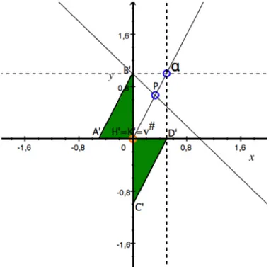
4.3. Cooperative solutions. The best way for the two players to get both a gain is to find a cooperative solution. One way would be to divide fairly the maximum collective profit W , determined by the maximum of the collective gain functional g, defined by g(X ,Y ) = X +Y , on the payoffs space of the game G, i.e the profit W = max_f(E×F)g. The maximum collective

profit W is attained at the point B′, which is the only bi-win belonging to the straight line g−1(1) (with equation g = 1) and to the payoff space f (E × F). So, ME and Bank play (1, 1), in order to arrive at the payoff B′. Then, they split the obtained bi-gain B′by means of a binding contract.

Financial point of view. ME buys futures to create artificially a misalignment between futures and spot prices; misalignment that is exploited by Bank, which get the maximum win W = 1. For a possible fair division of W = 1, we employ a transferable utility solution: finding on the transferable utility Pareto boundary of the payoff space a non-standard Kalai-Smorodinsky solution (non-standard because we do not consider the whole game, but only its maximal Pareto boundary). We find the supremum of maximal boundary,

sup ∂∗f(E × F),

which is the point α = (1/2, 1), and we join it with the infimum of maximal Pareto boundary, inf ∂∗f(E × F),

which is (0, 0). We note that the infimum of our maximal Pareto boundary is equal to v♯= (0, 0) (the conservative bi-gain of the game). The intersection point P, between the straight line of maximum collective win (i.e. (g = 1)) and the straight line joining the supremum of the maximal Pareto boundary with its infimum (i.e., the line Y = 2X ) is the desirable division of the maximum collective win W = 1 between the two players.

Figure 6 shows the situation.

The point P = (1/3, 2/3) suggests that ME should receive 1/3, by contract, from Bank, while at Bank remains the win 2/3.

5. Coopetitive approach

In order to consider our game as a remedy to the credit crunch problem, we pass from the game studied by Carfì and Musolino (2013c) to a game set in a coopetitive context. To this purpose, now we consider the new coopetitive approach introduced by Carfì. We have two players, ME and Bank, each of them has a strategy set in which to choose strategies; moreover, the two players can cooperatively choose a strategy z in a third set C. The two players choose their cooperative strategy z to maximize (in some sense we shall specify) the gain function f .

5.0.1. The shared strategy. Any strategy z ∈ [0, 1] is a shared strategy, which represents the percentage of the biggest amount of money M3(expressed in Euro) loanable to Bank by the ECB with a very low interest rate (hypothesis highly plausible given the recent anti-crisis measures adopted by the ECB), rate which, by convention we assume equal to 0. The two players want the loan so that ME can create an even higher misalignment between spot and futures price, misalignment which will be exploited by Bank. In this way, both players can get a greater win than that obtained without a shared strategy z.

The two players can then choose together a shared strategy z depending on they want: (1) to use not the money of the ECB (z = 0);

(2) to use a part of the money of the ECB, so that ME purchases futures (0 < z < 1); (3) to use totally the money of the ECB so that ME purchases futures (z = 1). 5.1. The payoff function of ME. In practice, to the previous payoff function f1of ME, that is the function defined by

f1(x, y) = −νM1(1 − x)y,

for every (x, y) in the bi-strategy space S, we must add the payoff-consequence v1(y, z) of the shared action z of the game, consisting in buying Euro futures contracts and selling them at time 1 (action decided by both players and performed by ME). In section 4, we have already chosen M1= 1 and ν = 1/2, and so we have

f1(x, y) = −(1/2)(1 − x)y,

for every (x, y) in the bi-strategy space S: this is the first component of the initial game we shall represent in the present paper.

5.1.1. Payoff consequence of the shared strategy. The payoff function addendum v1(y, z), of ME, is given by the quantity of Euro futures bought, that is the term zM3, where M3is the maximum possible loan (expressed in Euro futures contracts) by the ECB, multiplied by the difference

F1(x, y, z)u−1− F0,

between the Euro futures price at time 1 - when ME sells the futures - and the futures price at time 0 - when ME buys the Euro futures.

5.1.2. Intervention of the regulatory authority. Similarly to what happened to Bank in subsection 3.4.1, also ME has to pay a tax on the sale of the Euro futures contracts. We assume that this tax is equal to the impact of ME on the price of the Euro futures, in order to avoid speculative acts created by itself.

5.1.3. Construction of the payoff function. We have:

h1(x, y, z) = −νM1(1 − x)y + M3(F1(x, y, z)u−1− m(x + z) − F0)z (6) where

(1) zM3is the quantity of Euro futures purchased. We choose M3= 1, for sake of simplicity.

(2) m(x + z) is the normative tax paid by ME on the sale of futures, referred to the time 1. In keeping with the size of x, also z is a percentage.

(3) F1(x, y, z) is the Euro price of the futures market (established) at time 1, after ME has played its strategy x and the shared strategy z and after Bank has chosen to buy yM2on the spot market of Euros. The price F1(x, y, z) is given by

F1(x, y, z) = S1(y)u + mu(x + z), (7) where

S1(y) = (S0+ ny)u

is the Euro spot price (expressed in Euros) at time 1, and u = 1 + i is the factor of capitalization of interests. By m we denote the marginal coefficient that measures the impact of x and z on the price F1(x, y, z). The price F1(x, y, z) depends on x and z because, if ME buys futures with a strategy x ̸= 0 or z ̸= 0, the price F1 changes because an increase of Euro futures demand influences the Euro futures price. The value S1should be capitalized because it follows the fundamental relationship between futures and spot prices (see section 2). The value m(x + z) is also capitalized because the strategies x and z are played at time 0 but have effect on the Euro futures price at time 1.

(4) (1 + i)−1is the discount factor. F1(x, y, z) must be translated at time 1 because the money for the sale of futures are cashed at time 2.

(5) F0is the Euro futures price at time 0. It represents the price established at time 0 that has to be paid at time 1 in order to buy the good. It is given by F0= S0uT, where u = 1 + i is the capitalization factor with rate i. S0is, on the other hand, the spot price of the underlying asset at time 0. S0is a constant because it does not influence our strategies x, y and z.

5.1.4. The payoff function of ME. Recalling the above point (5), Eq.(6) and Eq.(7), we have (setting u := 1 + i, x′= 1 − x)

h1(x, y, z) = −νM1x′y+ zM3[((S0+ ny)u2+ m(x + z)u)u−1− m(x + z) − S0u], that is

5.2. The payoff function of Bank. In our initial non-coopetitive game, the payoff function of second player (already analyzed in the subsection 3.4) is

f2(x, y) = M2mxy,

for every (x, y) in the bi-strategy space S. We have already chosen M2= 2 and m = 1/2 (Carfì and Musolino2013c), so we have

f2(x, y) = xy,

for every (x, y) in the bi-strategy space S: this is the second component of the initial game we shall represent in the present paper.

The initial non-coopetitive payoff function of Bank at time 1 is given by the multiplication of the quantity of goods bought on the spot market, that is yM2, times the difference among: (1) the Euro futures price F1(x, y) (it is a price established at time 1 but cashed at time

2) transferred to time 1, that is

F1(x, y)u−1;

(2) the tax introduced by the normative authority on financial transactions in order to stabilize the financial markets;

(3) the Euro purchase price at time 0, say S0, capitalized at time 1 (in other words we are accounting for all balances at time 1).

But in our coopetitive game, instead of the Euro futures price F1(x, y), we have to consider the futures price F1(x, y, z) which takes into consideration the shared strategy z (in fact at time 0 ME buys the additional quantity zM3of Euro futures contracts than our initial non-coopetitive game, and the Euro futures price F1changes consequently).

The payoff function of Bank of our coopetitive game is defined by:

h2(x, y) = yM2(F1(x, y, z)u−1− νy − S0u), (9) where

(1) y is the percentage of goods that Bank purchases or sells on the spot market of the underlying;

(2) M2is the maximum amount of good that Bank can buy or sell on the spot market, according to its economic availability;

(3) S0is the price paid by Bank in order to buy Euros on spot market at time 0. S0is a constant because strategies x, y and z do not influence it.

(4) νy is the normative tax on the price of the Euro futures paid at time 1. We are assuming that the tax is equal to the incidence of the strategy y of Bank on the Euro spot price at time 1, that is

S1(y) = (S0+ ny)u.

(5) F1(x, y, z) is the price of the Euro futures market (established) at time 1, after ME has played its strategy x and the shared strategy z. The price F1(x, y, z) is given by

F1(x, y, z) = S1(y)u + mu(x + z), where

is the Euro spot price at time 1, and u = 1 + i is the factor of capitalization of interests. With m we intend the marginal coefficient that measures the impact of xand z on F1(x, y, z). F1(x, y, z) depends on x and z because, if ME buys Euro futures with a strategy x ̸= 0 or z ̸= 0, the price F1changes because an increase of Euro futures demand influences the Euro futures price. The value S1should be capitalized because it follows the fundamental relationship between futures and spot prices. The value m(x + z) is also capitalized because the strategies x and z are played at time 0 but have effect on the Euro futures price at time 1.

(6) (1 + i)−1is the discount factor. F1(x, y, z) must be translated at time 1, because the money for the sale of Euro futures are cashed at time 2.

5.2.1. The coopetitive payoff function of Bank. Recalling functions F1and f2, we have

h2(x, y, z) = yM2m(x + z), (10)

5.2.2. The coopetitive payoff function of the game. So, we have

h(x, y, z) = (−νM1(1 − x)y, M2mxy) + yz(M3ν , M2m), (11) for every strategy triple (x, y, z) of our coopetitive game. In this paper, we shall represent the following numerical case:

h(x, y, z) = (−(1/2)(1 − x)y, xy) + yz(1/2, 1).

In the following figures (Fig. 7, Fig. 8, and Fig. 9), we show the 3D representations of our game h in correspondence of the extreme valeues of the coopetitive parameter z (z = 0, z = 1).

FIGURE8. Game h(., 1).

5.3. The coopetitive translating vectors. We note immediately, that the new function it is the same payoff function f of the first game already studied (see Eq.(5)),

f(x, y) = (−νyM1(1 − x), yM2mx), translated by the vector function

v(y, z) := zy(M3ν , M2m).

Recalling that y ∈ [−1, 1] and z ∈ [0, 1], we see that the vector v(y, z) belongs to the 2-range [−1, 1](M3ν , M2m).

5.4. Coopetitive payoff space. Concerning the payoff space of our coopetitive game (h, >), we note a meaningful result. Before we state it, observe that, since any shared strategy z is positive:

(1) the part of the initial payoff space f (S≥) (where S≥is the part of S such that the second projection pr₂is greater than 0) is translated upwards, when we consider the transformation by the coopetitive extension h of f and the shared variable z is increasing;

(2) the part of the initial payoff space f (S≤) (where S≤is the part of S such that the second projection pr₂is less than 0) is translated downwards, when we consider the transformation by the coopetitive extension h of f and the shared variable z is increasing.

Proposition. Let S := [0, 1] × [−1, 1] and Q := S × [0, 1]. Then, the payoff space h(Q) is union of h(., 0)(S) and h(., 1)(S).

Proof.The strategy space S is the union of S≥:= [0, 1] × [0, 1] and S≤:= [0, 1] × [−1, 0]. We shall split the proof into two parts.

Part 1. We’ll show that the shared strategy that maximizes the wins when y ≥ 0 is always z = 1, that is, we’ll show that h(x, y, z) ≤ h(x, y, 1), for every y ≥ 0 and every x in E, i.e. (x, y) ∈ S≥. Recalling the definition of h, we have to show that

(−νyM1(1 − x), yM2mx) + yz(M3ν , M2m) ≤ (−νyM1(1 − x), yM2mx) + y(M3ν , M2m), that is

yz(M3ν , M2m) ≤ y(M3ν , M2m)

and therefore we have to prove that yz ≤ y, which is indeed verified for any y ≥ 0. We can show also that h(x, y, z) ≥ h(x, y, 0), for every y ≥ 0 and every x in E. Indeed, we have to show that

(−νyM1(1 − x), yM2mx) + yz(M3ν , M2m) ≥ (−νyM1(1 − x), yM2mx), that is

yz(ν, M2m) ≥ 0

and therefore yz ≥ 0, which is indeed verified for any y ≥ 0. Since, with x ∈ [0, 1] and y∈ [0, 1], we have

h(x, y, 0) ≤ h(x, y, z) ≤ h(x, y, 1),

we obtain that the payoff part h([0, 1]3) is included in the union of the images h(., 0)(S≥) and h(., 1)(S≥).

Part 2. We shall show that the shared strategy that maximizes the losses when y ≤ 0 is always z = 1, that is, we’ll show that h(x, y, z) ≥ h(x, y, 1), for every y ≤ 0 and every x in E, i.e. for every (x, y) ∈ S≤. Recalling the definition of h, we have to show that

(−νyM1(1 − x), yM2mx) + yz(M3ν , M2m) ≥ (−νyM1(1 − x), yM2mx) + y(M3ν , M2m), that is to say

yz(M3ν , M2m) ≥ y(M3ν , M2m)

and therefore we have to prove yz ≥ y, which is indeed verified for any y ≤ 0. We can show also that

h(x, y, z) ≤ h(x, y, 0), for every y ≤ 0 and every x in E. Indeed, we have to show that

(−νyM1(1 − x), yM2mx) + yz(M3ν , M2m) ≤ (−νyM1(1 − x), yM2mx), that is

yz(ν, M2m) ≤ 0,

that is equivalent to yz ≤ 0, which is indeed verified for any y ≤ 0. Since, when x ∈ [0, 1] and y ∈ [0, −1], we have

h(x, y, 1) ≤ h(x, y, z) ≤ h(x, y, 0),

we obtain that the payoff part h(S≤× [0, 1]) is included in the union of the images of h(., 1)(S≤) and h(., 0)(S≤). This completes the proof. ■

In Fig. 10, Fig. 11 and Fig. 12, we show the initial payoff space, the payoff space corresponding to the coopetitive strategy z = 1/2 and the final payoff space of the entire coopetitive game h seen as a dynamical path depending (or better parametrized) by the coopetitive strategy set C.

FIGURE11. The payoff space of the game h(., 1/2)

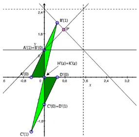
So, transforming our bi-strategic space S by h(., 0) (in dark green) and h(., 1) (in light green), in the Fig. 13 we have the whole of the payoff space of our coopetitive game (h, >). If ME Bank play the bi-strategy (1, 1) and the shared strategy 1, they arrive at the point B′(1), that is the maximum of the coopetitive game G, so ME wins 1/2 (amount greater than 1/3 obtained in the cooperative phase) while Bank wins even 2 (an amount much greater than 2/3, value obtained in the first cooperative phase).

FIGURE13. The payoff space of the coopetitive game h

5.5. Kalai-Smorodisky solution. Why a Kalai-Smorodinsky solution? The point B′(1) is the maximum payoff of the game (with respect to the usual component-wise order of the payoff plane). But ME could be not satisfied by the gain 1/2, value that is much more less than the win 2 of Bank. In addition, playing the shared strategy 1, ME increases only slightly the win obtained in the non-coopetitive game, on the contrary our Bank gains more than double.

For this reason, precisely to avoid that the possible dissatisfaction of ME can affect the game, Bank might be willing to cede part of its win by contract to the ME in order to balance the distribution of money, fairly.

Maximum collective gain. One way would be to distribute the maximum collective profitof the coopetitive game, that is the maximum value of the collective gain function

g: R2→ R : g(X,Y ) = X +Y, on the (compact) payoffs space of the game G, say

W = max h(Q)g.

The maximum collective profit is attained (evidently) at the maximum point point B′(1), which is the only bi-win belonging to the straight line g = 5/2 and to the payoff space. So ME and Bank play the coopetitive 3-strategy (1, 1, 1), in order to arrive at the payoff B′(1) and then split the wins obtained by contract. From a practical point of view:

ME buys futures to create artificially (also thanks to the money borrowed from the Eu-ropean Central Bank) a significant misalignment between Euro futures and spot prices, misalignment which is exploited by Bank getting the maximum win W= 5/2.

Fair division of the maximum collective gain. For a possible quantitative division of the maximum win W = 5/2, between Bank and ME, we propose a transferable utility Kalai-Smorodinsky method. The bargaining problem we face is the pair (Γ, B′(0)), where: (1) our decision constraint Γ is the transferable utility Pareto boundary of the

coopeti-tive game (straight line g = 5/2);

(2) we take, in our initial non-coopetitive game, the payoff with maximum possible collective profit, which is the point B′(0) = (0, 1), as threat point of our bargaining problem (the payoff B′(0) corresponds to the most likely Nash equilibrium of the initial non-coopetitive game (see Carfì and Musolino2013c).

Solution. For what concerns the solution: we join B′(0) with the supremum sup(Γ ∩ [B′(0), → [),

according to the classic Kalai-Smorodinsky method, supremum which is given by (5/2, 3/2). The coordinates of the intersection point P′, between the straight line of maximum collective gain (i.e. g = 2.5) and the segment joining B′and the considered supremum (the segment is part of the line (0, 1) + R(1, 1)) give us the desirable division of the maximum collective win W = 2.5, between the two players.

Figure 14 shows the procedure.

We obtain P′= (3/4, 7/4): ME receives 3/4 (more than double than the win obtained in the cooperative phase of the non-coopetitive game) by contract by Bank, while at Bank remains the win 7/4 (more than double than the win obtained in the cooperative phase of the non-coopetitive game).

6. Dynamical non-coopetitive interaction and generated fractal

After the initial non-coopetitive interaction, the two players decide to invest the obtained gains via the same method.

In this context the payoff functions are given, for every (x, y) ∈ E × F, by:

f1(x, y) = (−νy(1/3)M1(1 − x), y(1/3)M2mx) + (1/3, 2/3), (12) indeed the Kalai-Smorodinsky bi-gain of the initial game f0is P′:= (2/3)(νM1, mM₂) and the starting point is the Kalai-Smorodinsky w := P′= (1/3, 2/3) itself. We obtain the following Fig. 15.

FIGURE15. New payoff space f1(E × F).

Suppose to repeat the above strategic interaction, between the two operators, every year. We obtain the following recursive payoff functions:

fp(x, y) = (1/3)pf0(x, y) + (3/2)w(1 − (1/3)p) where, as we already know, f0is defined by:

f0(x, y) = (−(1/2)y(1 − x), xy), and

w:= (1/3, 2/3), for every time p in N.

We can represent this sequence of interactions by the following payoff evolution (see Fig. 16).

FIGURE16. Fractal-like payoff.

We also have implemented a software to represent the above payoff evolution, as shown in Fig. 17.

7. Conclusions

The games just studied suggests a possible regulatory model by which the phenomenon of the credit crunch (which in recent years determined the of crisis small and medium enterprises in Europe) should be greatly attenuated.

Moreover, the currency markets are stabilized through the introduction of a tax on financial transactions. In fact, in this way it could be possible to limit speculations.

Bank could:

• equally gain without taking advantage by speculative swings of currency prices; • and, specially, invest the money received by the ECB in the real economy lending

money to ME (which also gains something).

Non-coopetitive game. The unique sensible optimal solution is the cooperative one, otherwise the game appears like a sort of “your death, my life game”. This type of situation happens often in the economic competition and leaves no escapes if either player decides to work alone, without a mutual collaboration. In fact, all non-cooperative solutions lead to mediocre results for at least one of the two players.

We also study the dynamical evolution of a non-coopetitive interaction in time, assuming that the two operators reinvest the K-S gains every year in the same way. This evolution interaction leads us to a fractal object with an elusive point of convergence, which is, by the way, the supremum of the initial payoff space, circumstance very stimulating and of interest from an economic point of view.

Coopetitive game. Let us resume the results of the coopetitive approach.

(1) We can see that the game becomes much easier to solve in a satisfactory manner for both players.

(2) Moreover, the money received by the ECB are put into real economy by Bank: in fact, the bank (our second player) issues a loan for ME (our first player), which uses the money to buy Euros in order to hedge its Dollars credits.

(3) Both ME and Bank reduce their chances of losing with respect to the non-coopetitive game, and also they can easily reach to the maximum of the game: so ME wins 1/2 and Bank wins 2.

(4) If they take a transferable utility solution by the Kalai-Smorodisky method, ME increases the payout obtained in the non-coopetitive game (3/4 instead of 1/3), while Bank wins more of twice than before (7/4 instead of 2/3).

(5) We have moved from an initial competitive situation, that was not so profitable also acting in a cooperative way to a new coopetitive highly profitable situation both for ME and for Bank.

(6) We have also studied the dynamical evolution of a non-coopetitive interaction in time, assuming that the two operators reinvest the Kalai-Smorodinsky gains every year in the same way. This evolution interaction leads us to a fractal object with an elusive point of convergence, which is, by the way, the supremum of the initial payoff space, circumstance very stimulating and of great interest from an economic point of view.

References

Agreste, S., Carfì, D., and Ricciardello, A. (2012). “An algorithm for payoff space in C1parametric games”. Applied Sciences 14, 1–14.URL:http://www.mathem.pub.ro/apps/v14/A14-ag.pdf. Anonymous (2012). “Why the Euro Will Continue to Decline in Value Against the Dollar”. Economics

and Finance Fanatic.URL: http://www.economicsfanatic.com/2012/04/why-euro-will-continue-to-decline-in.html.

Arthanari, T., Carfì, D., and Musolino, F. (2015). “Game Theoretic Modeling of Horizontal Supply Chain Coopetition among Growers”. International Game Theory Review - Applied Optimization and Game-Theoretic Models. (in press).

Asch, S. E. (1952). Social Psycology. Englewood Cliffs, Prentice Hall.

Baglieri, D., Carfì, D., and Dagnino, G. (2010). “Profiting from Asymmetric R&D Alliances: Coopet-itive Games and Firm’s Strategies”. In: Proceedings of 4th Workshop on Coopetition Strategy “Coopetition and Innovation”, Montpellier, France, June 17-18, 2010. University of Montpellier

South of France and GSCM Montpellier Business School.

Baglieri, D., Carfì, D., and Dagnino, G. (2012). “Asymmetric R&D Alliances and Coopetitive Games”. In: Advances in Computational Intelligence, Part IV. 14th International Conference on Information Processing and Management of Uncertainty in Knowledge-Based Systems, IPMU 2012, Catania, Italy, July 9-13, 2012, Proceedings, Part IV. Ed. by S. Greco, B. Bouchon-Meunier, G. Coletti, M. Fedrizzi, B. Matarazzo, and R. Yager. Vol. 300. Communications in Computer and Information Science. Springer Berlin Heidelberg, pp. 607–621.DOI:10.1007/978-3-642-31724-8_64. Baglieri, D., Carfì, D., and Dagnino, G. (2015). “Asymmetric R&D Alliances: A Multi-Dimensional

Coopetitive Approach”. International Studies of Management and Organization. (in press). Carfì, D. (2008a). “Optimal boundaries for decisions”. Atti della Accademia Peloritana dei Pericolanti.

Classe di Scienze Fisiche, Matematiche e Naturali86(1), C1A0801002 [11 pages].DOI:10.1478/ C1A0801002.

Carfì, D. (2008b). “Superpositions in Prigogine’s approach to irreversibility for physical and finan-cial applications”. Atti della Accademia Peloritana dei Pericolanti. Classe di Scienze Fisiche, Matematiche e Naturali86(S1), C1S0801005 [13 pages].DOI:10.1478/C1S0801005.

Carfì, D. (2009a). “Complete study of linear infinite games”. In: Proceedings of the International Geometry Center. International Conference “Geometry in Odessa 2009”, 25-30 May 2009, Odessa, Ukraine. Vol. 2. 3, pp. 19–30.

Carfì, D. (2009b). “Decision-Form Games”. Communications to SIMAI Congress 3, 307, 1–12.DOI: 10.1685/CSC09307. Proceedings of the 9th Congress of SIMAI, the Italian Society of Industrial and Applied Mathematics, Roma (Italy), September 15-19, 2008.

Carfì, D. (2009c). “Differentiable game complete analysis for tourism firm decisions”. In: Proceedings of the 2009 International Conference on Tourism and Workshop on Sustainable tourism within High Risk areas of environmental crisis, Messina, Italy, April 22-25, 2009. University of Messina. SGB, pp. 1–10. Also available as MPRA paper 29193 athttp://mpra.ub.uni-muenchen.de/29193/. Carfì, D. (2009d). “Fibrations of financial events”. In: Proceedings of the International Geometry Center. International Conference “Geometry in Odessa 2009”, 25-30 May 2009, Odessa, Ukraine. Vol. 2. 3, pp. 7–18.

Carfì, D. (2009e). “Payoff space in C1Games”. Applied Sciences 11, 35–47.URL:http://www.mathem. pub.ro/apps/v11/A11-ca.pdf.

Carfì, D. (2010a). A model for coopetitive games. MPRA Paper 59633. University Library of Munich, Germany.URL:http://mpra.ub.uni-muenchen.de/59633/.

Carfì, D. (2010b). “The pointwise Hellmann-Feynman theorem”. Atti della Accademia Peloritana dei Pericolanti. Classe di Scienze Fisiche, Matematiche e Naturali88(1), C1A1001004 [14 pages].

Carfì, D. (2011). Financial Lie groups. MPRA Paper 31303. University Library of Munich, Germany.

URL:http://mpra.ub.uni-muenchen.de/31303/.

Carfì, D. (2012). “Coopetitive games and applications”. In: Advances and Applications in Game Theory - International Conference in honor of prof. Rao. Ed. by R. Mishra, S. Deman, M. Salunkhe, S. Rao, and J. Raveendran. Macmillan, pp. 128–147.

Carfì, D. and Cvetko-Vah, K. (2011). “Skew lattice structures on the financial events plane”. Applied Sciences13, 9–20.URL:http://www.mathem.pub.ro/apps/v13/A13-ca.pdf.

Carfì, D. and Fici, C. (2012). “The government-taxpayer game”. Theoretical and Practical Research in Economic Fields3(1(5)), 13–25.

Carfì, D., Gambarelli, G., and Uristani, A. (2013). “Balancing pairs of interfering elements”. Zeszyty Naukowe Uniwersytetu Szczeci`nskiego - Finanse, Rynki Finansowe, Ubezpieczenia760(59), 435– 442.

Carfì, D. and Lanzafame, F. (2014). “A Quantitative Model of Speculative Attack: Game Complete Analysis and Possible Normative Defenses”. In: Financial Markets: Recent Developments, Emerg-ing Practices and Future Prospects. Ed. by M. Bahmani-Oskooee and S. Bahmani. Nova Science. Chap. 9.

Carfì, D., Magaudda, M., and Schilirò, D. (2010). “Coopetitive game solutions for the eurozone economy”. In: Quaderni di Economia ed Analisi del Territorio. Quaderno n. 55/2010. Dipartimento DESMaS “V. Pareto” Università degli Studi di Messina. Il Gabbiano, pp. 1–21. Also available as MPRA paper 26541 athttp://mpra.ub.uni-muenchen.de/26541/.

Carfì, D. and Musolino, F. (2011a). “Fair Redistribution in Financial Markets: a Game Theory Complete Analysis”. Journal of Advanced Studies in Finance 2(2(4)), 74–100.

Carfì, D. and Musolino, F. (2011b). “Game complete analysis for financial markets stabilization”. In: Proceedings of the first international on-line conference on ‘Global Trends in Finance’. Ed. by R. Mirdala. Vol. 86. 1. ASERS Publishing House, pp. 14–42.URL:http://www.asers.eu/asers_ files/conferences/GTF/GTF_eProceedings_last.pdf.

Carfì, D. and Musolino, F. (2012a). “A Coopetitive Approach to Financial Markets Stabilization and Risk Management”. In: Advances in Computational Intelligence, Part IV. 14th International Conference on Information Processing and Management of Uncertainty in Knowledge-Based Systems, IPMU 2012, Catania, Italy, July 9-13, 2012, Proceedings, Part IV. Ed. by S. Greco, B. Bouchon-Meunier, G. Coletti, M. Fedrizzi, B. Matarazzo, and R. Yager. Vol. 300. Communications in Computer and Information Science. Springer Berlin Heidelberg, pp. 578–592.DOI: 10.1007/978-3-642-31724-8_62.

Carfì, D. and Musolino, F. (2012b). “Game theory and speculation on government bonds”. Economic Modelling29(6), 2417–2426.DOI:10.1016/j.econmod.2012.06.037.

Carfì, D. and Musolino, F. (2013a). “Credit Crunch in the Euro Area: A Coopetitive Multi-agent Solution”. In: Multicriteria and Multiagent Decision Making with Applications to Economics and Social Sciences. Ed. by A. G. S. Ventre, A. Maturo, ˘S. Ho˘skovà-Mayerovà, and J. Kacprzyk. Vol. 305. Studies in Fuzziness and Soft Computing. Springer Berlin Heidelberg, pp. 27–48.DOI: 10.1007/978-3-642-35635-3_3.

Carfì, D. and Musolino, F. (2013b). “Game theory application of Monti‘s proposal for European government bonds stabilization”. Applied Sciences 15, 43–70.URL:http://www.mathem.pub.ro/ apps/v15/A15-ca.pdf.

Carfì, D. and Musolino, F. (2013c). “Model of Possible Cooperation in Financial Markets in presence of tax on Speculative Transactions”. Atti della Accademia Peloritana dei Pericolanti. Classe di Scienze Fisiche, Matematiche e Naturali91(1), A3 [26 pages].DOI:10.1478/AAPP.911A3. Carfì, D. and Musolino, F. (2014). “Speculative and hedging interaction model in oil and U.S. dollar

markets with financial transaction taxes”. Economic Modelling 37, 306–319.DOI:10.1016/j. econmod.2013.11.003.

Carfì, D. and Musolino, F. (2015a). “Dynamical Stabilization of Currency Market with Fractal-like Trajectories”. Scientific Bulletin of the Politehnica University of Bucharest, Series A - Applied Mathematics and Physics. (in press).

Carfì, D. and Musolino, F. (2015b). “Tax Evasion: A Game Countermeasure”. Atti della Accademia Peloritana dei Pericolanti. Classe di Scienze Fisiche, Matematiche e Naturali. (to appear). Carfì, D., Musolino, F., Ricciardello, A., and Schilirò, D. (2012). “Preface: Introducing PISRS”. Atti

della Accademia Peloritana dei Pericolanti. Classe di Scienze Fisiche, Matematiche e Naturali 90(S1), E1 [4 pages].DOI:10.1478/AAPP.90S1E1.

Carfì, D., Musolino, F., Schilirò, D., and Strati, F. (2013). “Preface: Introducing PISRS (Part II)”. Atti della Accademia Peloritana dei Pericolanti. Classe di Scienze Fisiche, Matematiche e Naturali 91(S2), E1 [1 page].DOI:10.1478/AAPP.91S2E1.

Carfì, D., Patanè, G., and Pellegrino, S. (2011). “Coopetitive games and sustainability in Project Financing”. In: Moving from the crisis to sustainability. Emerging issues in the international context. Franco Angeli, pp. 175–182.

Carfì, D. and Perrone, E. (2011a). “Asymmetric Bertrand Duopoly: Game Complete Analysis by Algebra System Maxima”. In: Mathematical Models in Economics. Ed. by L. Ungureanu. ASERS Publishing House, pp. 44–66. Also available as MPRA paper 35417 athttp : / / mpra . ub. uni -muenchen.de/35417/.

Carfì, D. and Perrone, E. (2011b). “Game Complete Analysis of Bertrand Duopoly”. In: Mathematical Models in Economics. Ed. by L. Ungureanu. ASERS Publishing House, pp. 22–43.

Carfì, D. and Perrone, E. (2011c). “Game Complete Analysis of Bertrand Duopoly”. Theoretical and Practical Research in Economic Fields2 (1(3)), 5–22.

Carfì, D. and Perrone, E. (2012). Game complete analysis of symmetric Cournot duopoly. MPRA Paper 35930. University Library of Munich, Germany.URL:http://mpra.ub.uni-muenchen.de/35930/. Carfì, D. and Perrone, E. (2013). “Asymmetric Cournot Duopoly: A Game Complete Analysis”.

Journal of Reviews on Global Economics2, 194–202.DOI:10.6000/1929-7092.2013.02.16. Carfì, D. and Pintaudi, A. (2012). “Optimal Participation in Illegitimate Market Activities: Complete

Analysis of 2-Dimimensional Cases”. Journal of Advanced Research in Law and Economics 3(1(5)), 10–25.

Carfì, D. and Ricciardello, A. (2009). “Non-reactive strategies in decision-form games”. Atti della Accademia Peloritana dei Pericolanti. Classe di Scienze Fisiche, Matematiche e Naturali87(2), C1A0902002 [12 pages].DOI:10.1478/C1A0902002.

Carfì, D. and Ricciardello, A. (2010). “An algorithm for payoff space in C1-Games”. Atti della Accademia Peloritana dei Pericolanti. Classe di Scienze Fisiche, Matematiche e Naturali88(1), C1A1001003 [19 pages].DOI:10.1478/C1A1001003.

Carfì, D. and Ricciardello, A. (2012). “Topics in Game Theory”. Applied Sciences - Monographs (9).

URL:http://www.mathem.pub.ro/apps/mono/A-09-Car.pdf.

Carfì, D. and Ricciardello, A. (2013a). “An Algorithm for Dynamical Games with Fractal-Like Trajectories”. In: Fractal Geometry and Dynamical Systems in Pure and Applied Mathematics II: Fractals in Applied Mathematics. PISRS 2011 International Conference on Analysis, Fractal Geometry, Dynamical Systems and Economics, Messina, Italy, November 8-12, 2011 - AMS Special Session on Fractal Geometry in Pure and Applied Mathematics: in memory of Benoît Mandelbrot, Boston, Massachusetts, January 4-7, 2012 - AMS Special Session on Geometry and Analysis on Fractal Spaces, Honolulu, Hawaii, March 3-4, 2012. Ed. by D. Carfì, M. Lapidus, E. Pearse, and M. Van Frankenhuijsen. Vol. 601. Contemporary Mathematics. American Mathematical Society, pp. 95–112.DOI:10.1090/conm/601/11961.

Carfì, D. and Ricciardello, A. (2013b). “Computational representation of payoff scenarios in C1

Carfì, D. and Schilirò, D. (2011a). “Coopetitive games and global Green Economy”. In: Moving from the Crisis to Sustainability. Emerging Issues in the International Context. Franco Angeli, pp. 357–366.

Carfì, D. and Schilirò, D. (2011b). “Crisis in the Euro Area: Co-opetitive Game Solutions as New Policy Tools”. In: Mathematical Models in Economics. Ed. by L. Ungureanu. ASERS Publishing House, pp. 67–86.

Carfì, D. and Schilirò, D. (2011c). “Crisis in the Euro Area. Coopetitive Game Solutions as New Policy Tools”. Theoretical and Practical Research in Economic Fields 2(1(3)), 23–36.

Carfì, D. and Schilirò, D. (2012a). “A coopetitive model for the green economy”. Economic Modelling 29(4), 1215–1219.DOI:10.1016/j.econmod.2012.04.005.

Carfì, D. and Schilirò, D. (2012b). “A Framework of coopetitive games: Applications to the Greek crisis”. Atti della Accademia Peloritana dei Pericolanti. Classe di Scienze Fisiche, Matematiche e Naturali90(1), A1 [32 pages].DOI:10.1478/AAPP.901A1.

Carfì, D. and Schilirò, D. (2012c). “A Model of Coopetitive Game for the Environmental Sustainability of a Global Green Economy”. Journal of Environmental Management and Tourism 3(1(5)), 5–17. Carfì, D. and Schilirò, D. (2012d). “Global Green Economy and Environmental Sustainability: A Coopetitive Model”. In: Advances in Computational Intelligence. 14th International Conference on Information Processing and Management of Uncertainty in Knowledge-Based Systems, IPMU 2012, Catania, Italy, July 9-13, 2012, Proceedings, Part IV. Ed. by S. Greco, B. Bouchon-Meunier, G. Coletti, M. Fedrizzi, B. Matarazzo, and R. Yager. Vol. 300. Communications in Computer and Information Science. Springer Berlin Heidelberg, pp. 593–606.DOI: 10.1007/978-3-642-31724-8_63.

Carfì, D. and Schilirò, D. (2013). “A Model of Coopetitive Games and the Greek Crisis”. Contributions to Game Theory and Management6, 35–62.URL:http://www.gsom.spbu.ru/files/upload/gtm/ sbornik2012_27_05_2013.pdf. Collected papers presented on the Sixth International Conference Game Theory and Management, St. Petersburg, Russia, June 27-29, 2012.

Carfì, D. and Schilirò, D. (2014). “Coopetitive Game Solutions for the Greek Crisis”. In: Design a Pattern of Sustainable Growth. Innovation, Education, Energy and Environment. Ed. by D. Schilirò. ASERS Publishing House.

Carfì, D. and Trunfio, A. (2011). “A non-linear coopetitive game for global Green Economy”. In: Moving from the Crisis to Sustainability. Emerging Issues in the International Context. Franco Angeli, pp. 421–428.

Deutsch, M. and Gerard, H. (1955). “A Study of Normative and Informational Social Influences upon Individual Judgement”. Journal of Abnormal and Social Psychology (51(3)), 629–636.

Ford, J. L., Kelsey, D., and Pang, W. (2013). “Information and ambiguity: herd and contrarian behaviour in financial markets”. Theory and Decision 75(1), 1–15.DOI: 10.1007/S11238-012-9334-3.

Hull, J. C. (2002). Options, Futures and Other Derivatives. 5th edition. Prentice Hall.

Mediobanca (2012). Dati cumulativi di 2032 società italiane.URL:http://www.mediobanca.it/it/ stampa-comunicazione/news/mediobanca-pubblica-la-nuova-edizione-dei-dati-cumulativi-di-2032-societ-italiane.html.

Milgram, S. (1964). Obedience to Authority. Harper and Row.

Musolino, F. (2012). “Game theory for speculative derivatives: a possible stabilizing regulatory model”. Atti della Accademia Peloritana dei Pericolanti. Classe di Scienze Fisiche, Matematiche e Naturali 90(S1), C1 [19 pages].DOI:10.1478/AAPP.90S1C1.

Okura, M. and Carfì, D. (2014). “Coopetition and Game Theory”. Journal of Applied Economic Sciences9(3(29)), 457–468.URL:http://cesmaa.eu/journals/jaes/files/JAES_2014_Fall.pdf#page= 123.

Onaldo, M. (2012). “Rendimenti titoli di stato decennali a confronto”. lavoce.info.URL:http://www. lavoce.info/articoli/pagina1002823.html.

Palley, T. I. (1999). “Speculation and Tobin taxes: Why sand in the wheels can increase economic efficiency”. Journal of Economics 69(2), 113–126.DOI:10.1007/BF01232416.

Scharfstein, D. S. and Stein, J. C. (1990). “Herd Behavior and Investment”. The American Economic Review80(3), 465–479.URL:http://www.jstor.org/stable/2006678.

Wei, S.-J. and Kim, J. (1999). “The Big Players in the Foreign Exchange Market: Do They Trade on Information or Noise?” CID Working Paper No. 5.URL:http://www.hks.harvard.edu/content/ download/69265/1249870/version/1/file/005.pdf.

Westerhoff, F. and Dieci, R. (2006). “The effectiveness of Keynes-Tobin transaction taxes when heterogeneous agents can trade in different markets: A behavioral finance approach”. Journal of Economic Dynamics and Control30(2), 293–322.DOI:10.1016/j.jedc.2004.12.004.

a _{Department of Mathematics,}

Office: 271, Surge Math Building,

University of California, Riverside, CA 92521, USA

b _{Piazza Carso 11, 98121 Messina, Italy}

∗ _{To whom correspondence should be addresses | Email: david.carfi@ucr.edu}

Paper presented at the Permanent International Session of Research Seminars held at the DESMaS Department “Vilfredo Pareto” (Università degli Studi di Messina) under the patronage of the Accademia Peloritana dei Pericolanti

Communicated 16 September 2011; published online 27 February 2015

This article is an open access article licensed under aCreative Commons Attribution 3.0 Unported License