Gas-phase formation of Complex Organic Models molecules in interstellar medium: computational investigations

Scuola Normale Superiore di Pisa

GAS-PHASE FORMATION OF

COMPLEX ORGANIC MOLECULES IN

INTERSTELLAR MEDIUM:

COMPUTATIONAL INVESTIGATIONS

by Fanny Vazart

under the supervision of

Prof. Vincenzo Barone & Dr. Dimitrios Skouteris

A thesis presented for the degree of

Doctor of Philosophy

in Chemistry

2

Abstract

In the field of astro- and prebiotic chemistry, the building blocks of life, which are molecules composed of more than 6 atoms, are called Complex Organic Molecules (COMs). Their appearances on the early inorganic Earth is therefore one of the major issues faced by researchers interested in the origin of life. In this thesis, split into three parts, the main purpose is to show how different COMs are formed in interstellar medium (ISM), using computational chemistry.

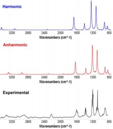
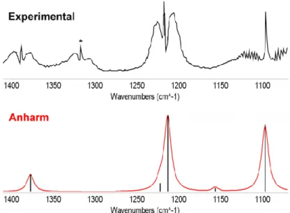
The first part focuses mainly on preliminary studies aiming at evaluating the appropriate level of theory to use to perform studies of formation reactions. First, a comprehensive benchmark of C≡N stretching vibrations computed at harmonic and anharmonic levels is reported with the goal of proposing and validating a reliable computational strategy to get accurate results for this puzzling vibrational mode, involved in biological molcules, without any ad hoc scaling factor. Anharmonic calculations employing second-order vibrational perturbation theory provide very good results when performed using the B2PLYP double-hybrid functional, in conjunction with an extended basis set and supplemented by semiempirical dispersion contributions. For larger systems, B2PLYP harmonic frequencies, together with B3LYP anharmonic corrections, offer a very good compromise between accuracy and computational cost without the need of any empirical scaling factor. As a second step, transition metal complexes are considered. Even though they have not been of primary importance in ISM so far, it is always useful to investigate a various range of compounds. Here, a quantum mechanical investigation on the luminescence properties of several mono- and dinuclear platinum(II) complexes and on an iridium(III) (d6 metal) complex is exhibited. The electronic structures and geometric parameters are briefly analyzed together with the absorption bands of all complexes. In all cases agreement with experiment is remarkable. Emission (phosphorescence) spectra from the first triplet states have also been investigated by comparing different computational approaches and taking into account also vibronic effects. Once again, agreement with experiment is good, especially using unrestricted electronic computations coupled to vibronic contributions. Together with the intrinsic interest of the results, the robustness and generality of the approach open the

3 opportunity for computationally oriented chemists to provide accurate results for the screening of large targets which could be of interest in molecular materials design.

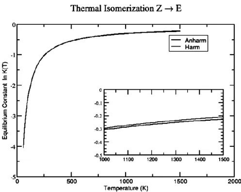
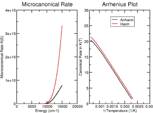
In the second part, new insights into the formation of several interstellar species of great relevance in prebiotic chemistry are provided by electronic structure and kinetic calculations. Cyanomethanimine isomers, formamide, glycolaldehyde and acetic acid are considered. (i) Concerning the first one, a full thermodynamic and vibrational investigation of C-cyanomethanimine isomers rooted into the Density Functional Theory (DFT) and the second-order vibrational perturbation theory (VPT2) is reported first. It is shown that an anharmonic treatment affects dramatically the vibrational behavior of the molecules, especially thanks to the inclusion of interaction terms between the various modes. Furthermore, the equilibrium constant between the isomers, as well as the rate constant, have been obtained at both harmonic and anharmonic levels showing, as expected, slight but non-negligible differences. Then, in order to solve the formation issue, the reaction CN + CH2=NH has been envisaged. This reaction is a facile formation route of Z,E-C-cyanomethanimine, even under the extreme conditions of density and temperature typical of cold interstellar clouds. E-C-cyanomethanimine has been recently identified in Sgr B2(N) in the Green Bank Telescope (GBT) PRIMOS survey and no efficient formation routes had been envisaged so far. The rate coefficients for the reaction channel show that the E-C-cyanomethanimine should be formed with a slightly lower yield than Z-C-E-C-cyanomethanimine. As the detection of E-isomer is favored due to its larger dipole moment, the missing detection of the Z-isomer can be due to the sensitivity limit of the GBT PRIMOS survey and the detection of the Z-isomer should be attempted with more sensitive instrumentation. The CN + CH2=NH reaction can also play a role in the chemistry of the upper atmosphere of Titan where the cyanomethanimine products can contribute to the buildup of the observed nitrogenrich organic aerosols that cover the moon. (ii) Concerning formamide, several pathways of the OH + CH2=NH and NH2 + H2CO reaction channels have been investigated. The results show that both reaction channels are essentially barrierless (in the sense that all relevant transition states lie below or only marginally above the reactants) and once tunneling is taken into proper account indicate that the reaction can occur under the low temperature conditions of interstellar environments. However, the OH + CH2=NH reaction tends to lead preferentially

4 to other products of prebiotic interest. Molecular deuteration has proven to be, in other cases, an efficient way to validate a synthesis route for molecules. For formamide, new published observations show that its three deuterated forms have all the same deuteration ratio. Following the work on the gas-phase formamide formation via the reaction NH2 + H2CO, new calculations of the rate cofficients for the production of monodeuterated formamide through the same reaction are presented, starting from monodeuterated NH2 or H2CO. The results of this new computations show that, at the 100 K temperature of the spot of interest, the rate of deuteration of the three forms is the same, within 20%. On the contrary, the reaction between non-deuterated species proceeds three times faster than that with deuterated ones. These results confirm that a gas-phase route for the formation of formamide is perfectly in agreement with the available observations. In order to further corroborate the results, new interferometric observations of formamide towards a recently shocked region near a young solar-type protostar is also reported. The new images of the molecular line emission show the spatial segregation of formamide with respect to other organic species. These observations, coupled with a chemical modelling analysis, provide new evidence that this potentially crucial brick of life can be efficiently formed in gas-phase around Sun-like protostars. (iii) Concerning glycolaldehyde and acetic acid, the precursors O(3_{P) and} hydroxyethyl radicals were considered (⦁CH₂CH₂OH for glycolaldehyde and CH_3⦁CHOH for acetic acid). Two reaction paths were obtained and the resulting rate constants show not only that they are viable in ISM, but also that when included in an astrochemical model, the obtained abundances for glycolaldehyde also match well the observed ones. In the case of acetic acid, the predicted abundances are too high compared to the observed ones.

To finish, the third part brings several miscellaneous studies together. The first one consists in a quick investigation on the glutamine rotamers, including the interconversion paths from one to the another. As far as it is concerned, the second one focuses on esterification in gas-phase. By mixing primary and secondary alcohols with carboxylic acids just before the supersonic expansion within pulsed Fourier transform microwave experiments, only the rotational spectrum of the ester was observed. However, when formic acid was mixed with tertiary alcohols, adducts were formed and their rotational spectra could be easily measured. Quantum mechanical calculations were therefore performed to

5 interpret the experimental evidence and the results are exhibited here. Finally, in the last study, the 1:1 complexes of ammonia with pyridine (i) and of tert-butyl alcohol with difluoromethane (ii) have been characterized by using state-of-the-art quantum-chemical computations combined with pulsed-jet Fourier-Transform microwave spectroscopy. (i) The computed potential energy landscape pointed out the formation of a stable σ-type complex, which has been confirmed experimentally: the analysis of the rotational spectrum showed the presence of only one 1:1 pyridine – ammonia adduct. The rotational spectrum provided the proof that the two molecules form a σ-type complex and that they are held together by both a N-H···N and a CH···N bond. This work represents the first application of an accurate and yet efficient computational scheme, designed for the investigation of small biomolecules, to a molecular cluster. Among the results obtained, the dissociation energy (BSSE and ZPE corrected) has been estimated to be 10.9 kJ·mol-1_{. (ii) The computed potential energy} landscape pointed out the formation of three stable isomers. However, the very low interconversion barriers explain why only one isomer, showing one O-H∙∙∙F and two C-H∙∙∙O weak hydrogen bonds, has been experimentally characterized.

6

Acknowledgements

I would like to thank all the people who contributed in some way to the work described in this thesis. First and foremost, I thank my academic advisor, Professor Vincenzo Barone, for accepting me into his group. During my tenure, he contributed to a rewarding PhD experience by giving me intellectual freedom in my work together with support and advice, supporting my attendance at various conferences and demanding a high quality of work in all my endeavors. Additionally, I would like to thank my committee members for their interest in my work.

Every result described in this thesis was accomplished with the help and support of fellow labmates and collaborators. Dr. Camille Latouche and I worked together on several different projects, particularly treating transition metal complexes, and without his efforts and pieces of advice, my job would have undoubtedly been more difficult. I greatly benefited from his keen scientific insight and his ability to introduce me to practical work. I was also fortunate to have the chance to work with Dr. Dimitrios Skouteris, who was the first person to suggest I work on astrochemistry. He was an extremely reliable source of practical scientific knowledge and I am grateful for his collaboration, particularly regarding the kinetics calculations described in this thesis. He also gave me the opportunity to meet Professors Nadia Balucani and Cecilia Ceccarelli whose knowledge in astronomy and astrochemistry were essential, and whose warm personalities were refreshing. They allowed me to attend a highly profitable and fascinating astrochemistry summer school and I am grateful for it. Last but not least, I would like to thank Professor Cristina Puzzarini for her help and collaboration in performing high-level computations and experiments related to the projects exhibited in this thesis.

Additionally, I would like to thank the various members of the DREAMS lab chemistry department with whom I had the opportunity to work and have not already mentioned: Dr. Nicola Tasinato, Dr. Serena Manti, Dr. Danilo Calderini, Dr. Julien Bloino and Nicola Fusè. They provided a friendly and cooperative atmosphere at work and also useful feedback and insightful comments on my work. I also had the opportunity to help a fellow PhD student, Dr. Ilaria Domenichelli, with some computations related to her project. I would be ingrate if I did not thank Monica Sanna, who deserves credit for providing much needed assistance with

7 administrative tasks and keeping our work running smoothly. Additionally, the Avogadro staff provided immediate support for any computer problems we encountered.

On another hand, I would like to acknowledge the Scuola Normale Superiore. My PhD experience benefitted greatly from the high-level courses I took and the high-quality seminars that the department organized.

Finally, I would like to acknowledge friends and family who supported me during my time here. First of all, I would like to thank David for his constant love and support, even when I had no time for him. I am also forever indebted to my parents for giving me the opportunities and experiences that have made me who I am. They selflessly encouraged me to explore new directions in life and this journey would not have been possible if not for them.

8

Contents

List of acronyms...p.12 Introduction...p.13

Kinetics and transition state theory...p.14 Theoretical details...p.16

PART I. Preliminary Studies

Computational details...p.30 Chapter 1. Accurate Infrared (IR) Spectra for Molecules Containing the C≡N Moiety by Anharmonic Computations with the Double Hybrid B2PLYP Density Functional...p.32

1.1. Specific computational details...p.33 1.2. Preliminary study...p.34 1.3. Full anharmonic treatment...p.35 1.4. Scaling factor and hybrid approach...p.37 1.5. Reduced dimensionality approach...p.39 1.6. IR spectral shape...p.39 1.7. Partial conclusion...p.41

Chapter 2. Transition Metal Complexes...p.42 2.1. Vibronic coupling investigation to compute phosphorescence spectra of Pt(II).p.42

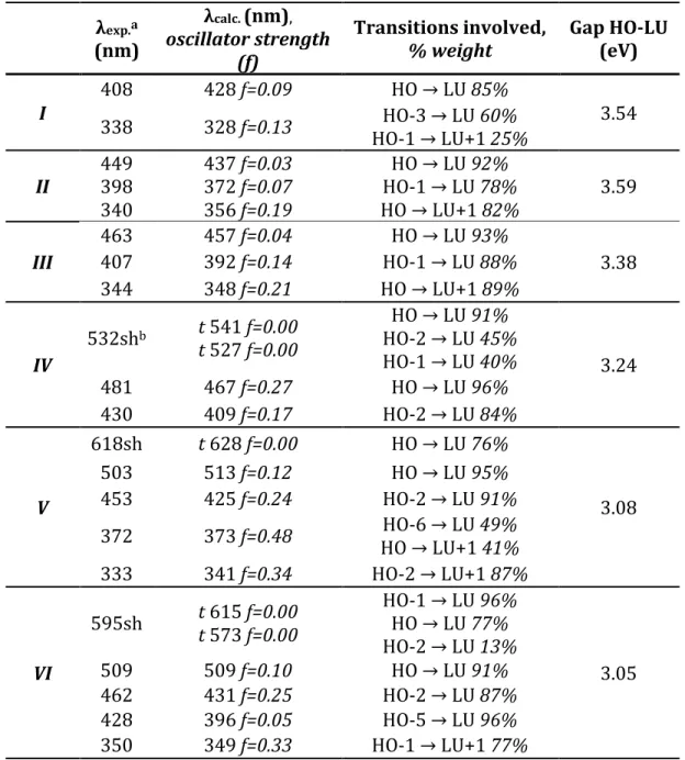
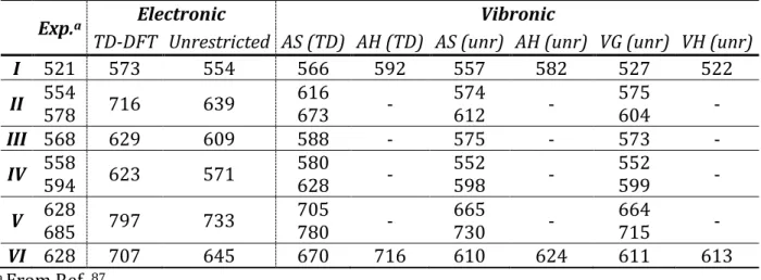
2.1.1. Specific computational details...p.43 2.1.2. Structural investigation...p.44 2.1.3. Absorption...p.45 2.1.4. Phosphorescence...p.47 2.1.5. Partial conclusion...p.52

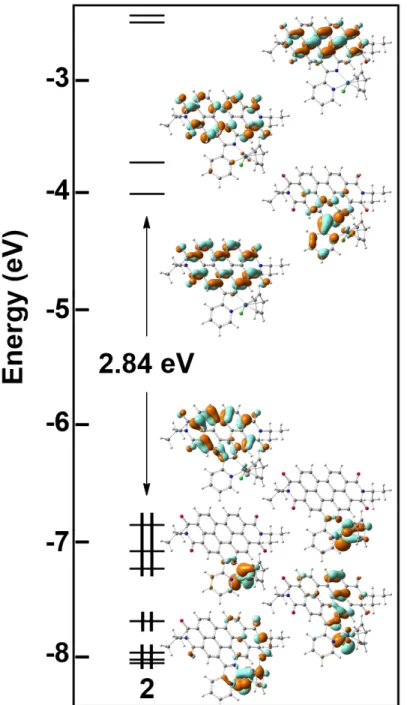
2.2. Validation of a computational protocol to simulate near IR phosphorescence spectra for an Ir(III) metal complex...p.53

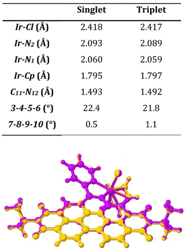
2.2.1. Specific computational details...p.54 2.2.2. Structural investigations...p.54 2.2.3. Electronic structure and vertical excitations...p.55 2.2.4. Excited states...p.57

9

2.2.5. Phosphorescence...p.58 2.2.6. Partial conclusion...p.59

PART II. Gas-phase Formation Routes for Complex Organic Molecules in

the Interstellar Medium

Computational details...p.60 Chapter 1. Cyanomethanimine isomers...p.61 1.1. Re-assessment of the thermodynamic, kinetic, and spectroscopic features of cyanomethanimine derivatives: a full anharmonic perturbative treatment...p.61

1.1.1. Specific computational details...p.62 1.1.2. Infrared investigations...p.65 1.1.3. Thermodynamics and kinetics...p.68 1.1.4. Partial conclusion...p.73

1.2. Cyanomethanimine isomers in cold interstellar clouds: insights from electronic structure and kinetic calculations...p.74

1.2.1. Specific computational details...p.76 1.2.2. Electronic structure calculations...p.78 1.2.3. Kinetics calculations...p.84 1.2.4. Partial conclusion...p.85

Chapter 2. The peculiar case of formamide...p.87 2.1. State-of-the-art thermochemical and kinetic computations for formamide formation in cold interstellar clouds...p.87

2.1.1. Specific computational details...p.88 2.1.2. Validation of structural and vibrational results...p.92 2.1.3. Choice of methodology...p.93 2.1.4. Mechanistic study...p.95 2.1.5. Kinetics study...p.106 2.1.6. Partial conclusion...p.110

2.2. Quantum chemical computations of formamide deuteration...p.111

10

2.2.2. Electronic structure and kinetics calculations...p.113 2.2.3. Comparison with astronomical observations...p.117 2.2.4. Partial conclusion...p.118

2.3. New observations as a support for gas-phase formation...p.119

2.3.1. Details of the observations...p.121 2.3.2. Astrochemical model: assumptions and results...p.123 2.3.3. Partial conclusion...p.126

Chapter 3. Astrochemical study of the formation of glycolaldehyde and acetic acid starting from ethanol...p.127

3.1. Specific computational details...p.129 3.2. Vibrational study of glycolaldehyde and acetic acid...p.129 3.3. Hydroxyethyl radicals...p.130 3.4. Electronic calculations...p.131 3.5. Kinetics study...p.137 3.6. Astrochemical modelling...p.138 3.7. Partial conclusion...p.140

PART III. Miscellaneous Investigations

Computational details...p.141 Chapter 1. Rotamers of glutamine...p.141

1.1. Specific computational details...p.142 1.2. Electronic structures...p.142 1.3. Interconversion paths...p.143 1.4. Partial conclusion...p.145

Chapter 2. Borderline between reactivity and pre-reactivity of binary mixtures of gaseous carboxylic acids and alcohols...p.146

2.1. Rotational spectra...p.147 2.2. Calculation details and results...p.149 2.3. Partial conclusion...p.152

11

Chapter 3. Interactions in organic complexes...p.153 3.1. Non-covalent interactions and internal dynamics in pyridine-ammonia: a combined quantum-chemical and microwave spectroscopy study...p.153

3.1.1. Computational details and results...p.154 3.1.2. Rotational spectrum...p.158 3.1.3. Dissociation energy...p.163 3.1.4. Partial conclusion...p.164

3.2. On the competition between weak O-H∙∙∙F and C-H∙∙∙F hydrogen bonds, in cooperation with C-H∙∙∙O contacts, in the difluoromethane – tert-butyl alcohol cluster...p.166

3.2.1. Computational details...p.167 3.2.2. Experimental methods and Rotational spectrum...p.170 3.2.3. Results...p.171 3.2.4. Partial conclusion...p.175

General Conclusions...p.176 References...p.178 Publication list...p.204

12

List of acronyms

COM Complex Organic Molecule

DFT Density Functional Theory

FA Formic Acid

ISM InterStellar Medium

PES Potential Energy Surface

PCM Polarizable Continuum Model

TD-DFT Time-Dependent Density Functional Theory

13

Introduction

How did life appear on an originally inorganic Earth? This is the main question which is faced by prebiotic chemists and astrochemists. As a rocky planet, Earth is mostly composed of rocks and metals and at its early stages, no organic compound could be found at its surface. However, between 3.8 and 4.1 billion years ago, life arose. In order for it to appear, the presence of water was mandatory. This explains why its origin on Earth has been widely investigated.1–4 _{Two main scenarios emerged from these studies: an extraterrestrial origin} hypothesis and an out-gassing scenario. The first one would consist in an arrival of water on Earth carried by comets or asteroids while the second implies that water was already present inside Earth during its formation and was released by volcanic activity. In the field of prebiotic chemistry and astrochemistry, the simplest organic building blocks for life, such as amino or nucleic acids and their possible precursors, are called Complex Organic Molecules (COMs) and usually contain up to around 10 atoms. Considering that many of these species have been detected in the interstellar medium (ISM), the most widespread hypothesis to explain how they were brought to Earth involves a transportation of these compounds on comets or asteroids,5–8_{like in the first scenario for the origin of water.The Rosetta spacecraft} was recently able to detect some COMs in the dust surrounding its target comet (67p), which strengthens the argument that the building blocks of life itself may have come from icy space rocks.9 _{As an example of these COMs, one could cite formamide, the simplest amide, which} can be considered a precursor in the abiotic amino acid synthesis and perhaps also that of nucleic acid bases.10–12 _{It can be therefore considered as a central compound that could} connect both metabolism –conversion of energy, ruled by proteins– and genetics –passage of information, ruled by DNA and RNA–. Glycolaldehyde and glycine are also of major importance as the first detected interstellar sugar molecule and amino acid, respectively. Indeed, as glycolaldehyde has been detected in ISM,13 _{glycine has been found in comets and} asteroids.14

The question of their formation is thus a burning issue. As a matter of fact, two main theories are now discussed to explain how chemical reactions can occur at very low densities –pressure– and temperature environments: dust grain and gas phase chemistry. The first one relies on surface reaction mechanisms and can allow to lower some reaction barriers –which

14 could have kept the reaction from happening at very low temperatures– and to ease the encounter between reactants –which can be difficult at very low pressures–. However, this theory faces some major issues, such as the adsorption/desorption mechanisms. Indeed, if we take a look at the formation of methanol for example, it is commonly believed that it occurs on the surface of dust grains.15,16_{Yet, this molecule was detected also in gas phase in} several cold and dark zones where no thermal desorption or photodissociation can follow.17,18 _{This problem led to doubt this surface formation mechanism. In order to avoid} those problems, one can consider the second theory: gas-phase reaction routes. In that case, there is not any desorption to consider but the proposed reaction mechanisms cannot involve any barrier and the only available energy is the one issuing from the reactants. Furthermore, no three body collision can be envisaged. This work will focus exclusively on gas-phase reactions.

The formation of COMs in ISM is a very complicated topic that requires three different types of expertise: observation, experiments and theoretical calculations. Astronomers, experimental and theoretical chemists should therefore work together in order to match the different locations where some compounds can be detected with the possible formation mechanisms. Another obstacle that can arise is the difficulty of reproducing experimentally the harsh conditions of the interstellar medium; accordingly, theoretical calculations are mandatory. It is then possible, once the reaction channels issuing from reactants are determined, to calculate as well the reaction rates for the formation of the products depending on the temperature. With these reaction rates, some astrochemical models are set up in order to obtain calculated abundances of the products, which are then feasibly compared with measured abundances in zones that can exhibit different temperatures.

Kinetics and transition state theory

Chemical kinetics is the study of rates of chemical processes. These reaction rates for a reactant or a product can explain how quickly a reaction takes place. They strongly depend on several factors, including temperature, pressure and concentration.

When considering the basic reaction:

15 The reaction rate can be defined as:

𝑟 = −

1

𝑎

𝑑[𝐴]

𝑑𝑡

= −

1

𝑏

𝑑[𝐵]

𝑑𝑡

=

1

𝑐

𝑑[𝐶]

𝑑𝑡

=

1

𝑑

𝑑[𝐷]

𝑑𝑡

where [X] stands for the concentration of X.

It is also possible to consider the rate equation, a mathematical expression that links the rate of a reaction to the concentrations of the reactants, of the form:

𝑟 = 𝑘(𝑇)[𝐴]

[𝐵]

here, n and m are the reaction orders, which can be different from the stoichiometric coefficients and depend on the reaction mechanism. k(T), as far as it is concerned, is the reaction rate coefficient, or rate constant. It is not really a constant because it depends on the temperature, often described by the Arrhenius equation:

𝑘(𝑇) = 𝐴𝑒

where A is a pre-exponential factor, R is the gas constant and Ea the activation energy of the

reaction.

In order to understand the physical meaning of Ea, one should consider the transition

state theory. This theory is based on three basic ideas:

(i) Rates of reaction can be studied by examining activated complexes near the saddle point of a potential energy surface, the details of how these complexes are formed not being important. The saddle point is called the transition state (TS).

(ii) The activated complex is in quasi-equilibrium with the reactant molecules.

(iii) The activated complex can convert into products, and kinetic theory can be used

to calculate the rate of this conversion.

In the particular case exhibited in Figure 1a, this single-step reaction is exothermic since the energy of the products is lower than the energy of the reactants. The endothermic reaction (products higher in energy than reactants) could have been considered as well. In both cases, the TS is always higher in energy than both reactants and products. One can also consider multi-step reactions, such as shown in Figure 1b. Here, all TSs are more energetic than both minima (reactants, reaction intermediates, products) they link.

(1)

(2)

16

a b

Figure 1. Basic reaction coordinates diagrams.

Theoretical details

Most of the calculations presented here are based on the Density Functional Theory (DFT).

The Schrödinger equation

In quantum chemistry, the ultimate goal is to solve the time-independent non-relativistic Schrödinger equation:

𝐻

̂𝛹

(𝑥

⃗⃗⃗ , 𝑥

⃗⃗⃗⃗ , … , 𝑥

⃗⃗⃗⃗ , 𝑅

⃗⃗⃗⃗ , 𝑅

⃗⃗⃗⃗ , … , 𝑅

⃗⃗⃗⃗⃗ ) = 𝐸

𝛹

(𝑥

⃗⃗⃗ , 𝑥

⃗⃗⃗⃗ , … , 𝑥

⃗⃗⃗⃗ , 𝑅

⃗⃗⃗⃗ , 𝑅

⃗⃗⃗⃗ , … , 𝑅

⃗⃗⃗⃗⃗ )

Ψ being the wave function and 𝐻̂ the Hamiltonian for a system that consists in M nuclei and

N electrons. Starting from here, atomic units are used.

𝐻

̂ = −

1

2

∑ ∇

−

1

2

∑

1

𝑀

∇

− ∑ ∑

𝑍

𝑟

+ ∑ ∑

1

𝑟

+ ∑ ∑

𝑍

𝑍

𝑅

here, the first two terms describe the kinetic energy of the electrons and nuclei while the three following terms represent the attractive electrostatic interaction between the nuclei and the electrons, the repulsive potential due to the electron-electron and nucleus-nucleus interactions.

In order to simplify Eq. 2, one can use the Born-Oppenheimer approximation that considers the electrons moving in the field of fixed nuclei. It is based on the fact that the masses of electrons are much lower than the masses of nuclei, which leads the latter to move much slower than the former. Thanks to this approximation, the nuclear kinetic energy is

Reaction coordinates Ener gy _{A + B} C + D Transition state Ea Reaction coordinates Ener gy _{A + B} C + D TS1 TS2 intermediate (1) (2)

17 zero and the potential energy of nuclei is merely a constant, which reduces the electronic Hamiltonian to:

𝐻

̂

= −

1

2

∑ ∇

− ∑ ∑

𝑍

𝑟

+ ∑ ∑

1

𝑟

= 𝑇̂ + 𝑉̂

+ 𝑉̂

The solution of the Schrödinger equation using 𝐻̂_{𝑒𝑙𝑒𝑐} is the electronic wave function Ψelec and

the electronic energy Eelec. The total energy Etot is then the sum of Eelec and Enuc, the constant

nuclear repulsion term.

𝐻

̂

𝛹

= 𝐸

𝛹

𝐸

= 𝐸

+ 𝐸

𝐸

= ∑

∑

The variational principle for the ground state

When a system is in the state Ψ, the expectation value of the energy is given by:

𝐸[𝛹] =

𝛹

𝐻

̂

_𝛹

⟨

𝛹

𝛹

⟨𝛹|𝐻

̂|𝛹⟩ = ∫ 𝛹

∗

_𝐻

_{̂𝛹𝑑𝑥}

The variational principle states that the energy computed from a guessed Ψ is an upper bound to the true ground-state energy E0. Full minimization of the functional E[Ψ] with

respect to all allowed N-electron wave functions will give the true ground state Ψ0 and energy

E[Ψ0] = E0, that is:

𝐸

= 𝑚𝑖𝑛

𝐸[Ψ] = 𝑚𝑖𝑛

⟨Ψ|𝑇̂ + 𝑉̂

+ 𝑉̂

|Ψ⟩

For a system of N electrons and given nuclear potential Vext, the variational principle

defines a procedure to determine the ground-state wave function Ψ0, the ground-state energy

E0[N,Vext], and other properties of interest. It needs to be noted that Ψ0 must be antisymmetric

with respect to electrons. In other words, the ground state energy is a functional of the number of electrons N and the nuclear potential Vext:

𝐸

= 𝐸[𝑁, 𝑉

]

18

The Hartree-Fock approximation

Supposing that Ψ0 is approximated as an antisymmetrized product of N orthonormal

spin orbitals 𝜓_𝑖(𝑥 ), each a product of a spatial orbital 𝛷𝑘(𝑟 ) and a spin function σ(s) = α(s) or β(s), the following Slater determinant is obtained:

Ψ

≈ Ψ

=

1

√𝑁!

||

…

…

⋮

⋮

⋱

…

||

The Hartree-Fock approximation is the method whereby the orthogonal orbitals ψi

are searched to minimize the energy for this determinantal form of Ψ0:

𝐸

= 𝑚𝑖𝑛

𝐸[Ψ

]

The expected value of energy EHF using the Hamiltonian operator is given by:

𝐸

= ⟨𝛹

|𝐻

̂|𝛹

⟩ = ∑ 𝐻

+

1

2

∑ (𝐽

+ 𝐾

)

𝐻

= ∫

(

) [−

1

2

∇

_{+ 𝑉}

(𝑥 )]

(𝑥 )𝑑𝑥

which defines the contribution due to the kinetic energy and the electron-nucleus attraction.

𝐽

= ∫ ∫ 𝜓

(𝑥

⃗⃗⃗ )𝜓

(𝑥

⃗⃗⃗ )

1

𝑟

𝜓

∗

_(𝑥

⃗⃗⃗⃗ )𝜓

(𝑥

⃗⃗⃗⃗ )𝑑𝑥

⃗⃗⃗ 𝑑𝑥

⃗⃗⃗⃗

are the Coulomb integrals and

𝐾

= ∫ ∫ 𝜓

(𝑥

⃗⃗⃗ )𝜓

(𝑥

⃗⃗⃗ )

1

𝑟

𝜓

(𝑥

⃗⃗⃗⃗ )𝜓

(𝑥

⃗⃗⃗⃗ )𝑑𝑥

⃗⃗⃗ 𝑑𝑥

⃗⃗⃗⃗

are the exchange integrals.

𝐽

≥ 𝐾

≥ 0

𝐽

= 𝐾

The minimization of the energy functional of Eq. 11, together with the normalization conditions ∫ 𝜓𝑖∗(𝑥 )𝜓𝑗(𝑥 ) 𝑑𝑥 = 𝛿𝑖𝑗 lead to the Hartree-Fock differential equations:

(9) (10) (11) (12) (13) (14)

19

𝑓̂𝜓

= 𝜖

𝜓

, i=1, 2, …, N

The Fock operator 𝑓̂ is an effective one-electron operator defined as:

𝑓̂ = −

1

2

∇

_{− ∑}

𝑍

𝑟

+ 𝑉̂

(𝑖)

The first two terms represent the kinetic energy and the potential energy due to the electron-nucleus attraction. 𝑉̂_𝐻𝐹(𝑖), as far as it is concerned, is the Hartree-Fock potential operator, the average repulsive potential experienced by the ith _{electron due to the remaining}

N-1 electrons, and is given by:

𝑉̂

(𝑥

⃗⃗⃗ ) = ∑(𝐽̂

(𝑥

⃗⃗⃗ ) − 𝐾

̂

(𝑥

⃗⃗⃗ ))

𝑁

𝑗

with the Coulomb operator 𝐽̂ that represents the potential an electron at position 𝑥 1experiences due to the average charge distribution of another electron in spin orbital ψj, defined as:

𝐽̂

(𝑥

⃗⃗⃗ ) = ∫|𝜓

(𝑥

⃗⃗⃗⃗ )|²

1

𝑟

𝑑𝑥

⃗⃗⃗⃗

and 𝐾̂ that is the exchange contribution to the HF potential and is defined through its effect when operating on a spin orbital:

𝐾

̂

(𝑥

⃗⃗⃗ )𝜓

(𝑥

⃗⃗⃗ ) = ∫ 𝜓

(𝑥

⃗⃗⃗⃗ )

1

𝑟

𝜓

(𝑥

⃗⃗⃗⃗ )𝑑𝑥

𝜓

(𝑥

⃗⃗⃗ )

The HF potential is non-local and depends on the spin orbital. Therefore, the HF equations must be solved self-consistently. Moreover, the Koopman's theorem provides a physical interpretation of the orbital energies: it states that the orbital energy εi is an approximation of minus the ionization energy associated with the removal of an electron from the orbital ψi, i.e. 𝜖_𝑖 ≈ 𝐸_𝑁− 𝐸_𝑁−1𝑖 = −𝐼𝐸(𝑖).

The electron density

The electron density 𝜌(𝑟 ) is a central property in DFT and is defined as the integral over the spin coordinates of all electrons and over all but one spatial variables. It determines the probability of finding an electron (among the N) within the volume element 𝑑𝑟 .

(15)

(16)

(17)

(18)

20

𝜌(𝑟 ) = 𝑁 ∫ … ∫|𝛹(𝑥

, 𝑥

, … , 𝑥

)|

𝑑𝑠

𝑑𝑥

⃗⃗⃗⃗ … 𝑑𝑥

⃗⃗⃗⃗

𝜌(𝑟 ) is a non-negative function of only the three spatial variables (as opposite to Ψ, that depends on 4N variables) that vanishes at infinity and integrates to the total number of electrons:

𝑙𝑖𝑚

𝜌(𝑟 ) = 0

∫ 𝜌(𝑟 )𝑑𝑟 = 𝑁

At any position of an atom, the gradient of 𝜌(𝑟 ) has a discontinuity and a cusp results:

𝑙𝑖𝑚

[∇

+ 2𝑍

]𝜌̅(𝑟 ) = 0

where Z is the nuclear charge and 𝜌̅(𝑟 ) the spherical average of 𝜌(𝑟 ).

The asymptotic exponential decay for large distance from all nuclei leads to this approximation:

𝜌(𝑟 )~exp⁡[−2√2𝐼|𝑟 |

The Thomas-Fermi model

This model can be considered the first density functional theory. It is based on the uniform electron gas and uses the following functional for the kinetic energy:

𝑇

[𝜌(𝑟 )] =

3

10

(3𝜋

2

₎

_{∫ 𝜌}

_{(𝑟 )𝑑𝑟}

The approximate energy of an atom is then obtained using the classical expression for the nuclear-nuclear potential and the electron-electron potential:

𝐸

[𝜌(𝑟 )] =

3

10

(3𝜋

₎

_{∫ 𝜌}

_{(𝑟 )𝑑𝑟 − 𝑍 ∫}

𝜌(𝑟 )

𝑟

𝑑𝑟 +

1

2

∫ ∫

𝜌(𝑟

)𝜌(𝑟

)

𝑟

𝑑𝑟

𝑑𝑟

This energy is completely given in terms of electron density.

In order to determine the correct density to be included in Eq. 25, a variational principle is employed. The ground state of the system is assumed to be connected to the 𝜌(𝑟 ) for which the energy is minimized under the constraint of ∫ 𝜌(𝑟 )𝑑𝑟 = 𝑁. However, this variational principle is not necessarily justified.

(20) (21) (22) (23) (24) (25)

21

The first Hohenberg-Kohn theorem

This theorem demonstrates that the electron density uniquely determines the Hamiltonian operator and thus all the properties of the system. It states that the external potential 𝑉_𝑒𝑥𝑡(𝑟 ) is (to within an additive constant) a unique functional of 𝜌(𝑟 ); since 𝑉_𝑒𝑥𝑡(𝑟 ) fixes 𝐻̂, the full many particle ground state is then a unique functional of 𝜌(𝑟 ).

Proof: if we assume that there were two external potentials 𝑉𝑒𝑥𝑡(𝑟 ) and 𝑉′𝑒𝑥𝑡(𝑟 ) differing by more than a constant, each giving the same 𝜌(𝑟 ) for its ground state, we would have two Hamiltonians 𝐻̂ and 𝐻̂′ whose ground-state densities were the same although the normalized wave functions Ψ and Ψ’ would be different. Taking Ψ’ as a trial wave function for the 𝐻̂ problem, we get:

𝐸

< ⟨𝛹’|𝐻

̂|𝛹’⟩ = ⟨𝛹’|𝐻′

̂|𝛹’⟩ + ⟨𝛹’|𝐻̂ − 𝐻′

̂|𝛹’⟩

= 𝐸′

+ ∫ 𝜌(𝑟 )[𝑉

(𝑟 ) − 𝑉

𝑒𝑥𝑡

(𝑟 )]𝑑𝑟

where 𝐸₀ and 𝐸′₀ are the ground-state energies for 𝐻̂ and 𝐻̂′, respectively. Similarly, taking

Ψ as a trial wave function for the 𝐻′̂ problem, we get:

𝐸′

< ⟨𝛹|𝐻′

̂|𝛹⟩ = ⟨𝛹|𝐻̂|𝛹⟩ + ⟨𝛹|𝐻′

̂ − 𝐻̂|𝛹⟩

= 𝐸

+ ∫ 𝜌(𝑟 )[𝑉

(𝑟 ) − 𝑉

𝑒𝑥𝑡

(𝑟 )]𝑑𝑟

Adding Eq. 26 and 27, we get 𝐸₀+ 𝐸′₀ < 𝐸′₀+ 𝐸₀, which is a contradiction. Therefore, there cannot be two different 𝑉𝑒𝑥𝑡(𝑟 ) that give the same 𝜌(𝑟 ) for their ground states.

Thus, 𝜌(𝑟 ) determines N and 𝑉_𝑒𝑥𝑡(𝑟 ) and hence all the properties of the system, for example the kinetic energy 𝑇[𝜌], the potential energy 𝑉[𝜌] and the total energy 𝐸[𝜌]. Now, the total energy can be written as:

𝐸[𝜌] = 𝐸

[𝜌] + 𝑇[𝜌] + 𝐸

[𝜌] = ∫ 𝜌(𝑟)𝑉

(𝑟)𝑑𝑟 + 𝐹

[𝜌]

𝐹

[𝜌] = 𝑇[𝜌] + 𝐸

This functional 𝐹_𝐹𝐾[𝜌] is the holy grail of density functional theory. If it were known, the Schrödinger equation could be solved exactly. And, since it is a universal functional completely independent of the system at hand, it applies equally well to the hydrogen atom (26)

(27)

(28) (29)

22 as to gigantic molecules. 𝐹_𝐹𝐾[𝜌] contains the functional for the kinetic energy 𝑇[𝜌] and that for the electron-electron interaction, 𝐸𝑒𝑒[𝜌]. The explicit form of both these functional is completely unknown. However, from the latter it is possible to extract at least the classical part 𝐽[𝜌]:

𝐸

[𝜌] =

1

2

∫ ∫

𝜌(𝑟

)𝜌(𝑟

)

𝑟

𝑑𝑟

𝑑𝑟

+ 𝐸

= 𝐽[𝜌] + 𝐸

[𝜌]

𝐸_𝑛𝑐𝑙 is the non-classical contribution to the electron-electron interaction: self-interaction correction, exchange and Coulomb correlation.

The explicit forms of the functionals 𝑇[𝜌] and 𝐸_𝑛𝑐𝑙[𝜌] is the major challenge of DFT.

The second Hohenberg-Kohn theorem

The second H-K theorem states that 𝐹_𝐹𝐾[𝜌], the functional that delivers the ground state energy of the system, delivers the lowest energy if and only if the input density is the true ground state density. This is also the variational principle:

𝐸

≤ 𝐸[𝜌̃] = 𝑇[𝜌̃] + 𝐸

[𝜌̃] + 𝐸

[𝜌̃]

In other words, for any trial density 𝜌̃(𝑟 ), which satisfies the necessary boundary conditions such as 𝜌̃(𝑟 ) ≥ 0, ∫ 𝜌̃(𝑟 )𝑑𝑟 = 𝑁, and which is associated with some external potential 𝑉̃_𝑒𝑥𝑡, the energy obtained from the functional of Eq. 28 represents an upper bound to the true ground state energy E0.

Proof: it makes use of the variational principle established for wave functions. We

recall that any trial density 𝜌̃ defines its own Hamiltonian 𝐻̂ and hence its own wave function 𝛹̃. This wave function can now be taken as the trial wave function for the Hamiltonian generated from the true external potential 𝑉_𝑒𝑥𝑡. Thus,

⟨𝛹

̃|𝐻̂|𝛹

̃⟩ = 𝑇[𝜌̃] + 𝐸

[𝜌̃] + ∫ 𝜌̃(𝑟 )𝑉

𝑑𝑟 = 𝐸[𝜌̃] ≥ 𝐸

[𝜌̃] = ⟨𝛹

̃

|𝐻

̂|𝛹

̃

⟩

The Kohn-Sham equations

The ground state energy of a system can be written as:

𝐸

= 𝑚𝑖𝑛

(𝐹[𝜌] + ∫ 𝜌(𝑟 )𝑉

𝑑𝑟 )

(31)

(32)

(33) (30)

23 where the universal functional 𝐹[𝜌] contains the contributions of the kinetic energy, the classical Coulomb interaction and the non-classical portion:

𝐹[𝜌] = 𝑇[𝜌] + 𝐽[𝜌] + 𝐸

[𝜌]

Here, only 𝐽[𝜌] is known. The main problem is to find the expressions for 𝑇[𝜌] and 𝐸_𝑛𝑐𝑙[𝜌].

The Thomas-Fermi model described above provides an example of density functional theory. However, its performance is really low due to the poor approximation of the kinetic energy. To solve this problem, Kohn and Sham proposed an alternative approach.

They suggested to calculate the exact kinetic energy of a non-interacting reference system with the same density as the real, interacting one:

𝑇

= −

2

∑ ⟨𝜓

|∇²|𝜓

⟩

𝑖

𝜌

(𝑟 ) = ∑ ∑ |𝜓

(𝑟 , 𝑠)| = 𝜌(𝑟 )

where the ψi are the orbitals of the non-interacting system. TS is not equal to the true kinetic

energy of the system but Kohn and Sham accounted for that by introducing the following separation of the functional 𝐹[𝜌] :

𝐹[𝜌] = 𝑇

[𝜌] + 𝐽[𝜌] + 𝐸

[𝜌]

where EXC, the so-called exchange-correlation energy is defined, thanks to Eq. 36, as:

𝐸

[𝜌] = (𝑇[𝜌] − 𝑇

[𝜌]) + (𝐸

[𝜌] − 𝐽[𝜌])

This EXC is the functional that contains everything that is unknown.

Now, the question is: how can we uniquely determine the orbitals in our non-interacting reference system? In other words, how can we define a potential VS such that it

provides us with a Slater determinant which is characterized by the same density as our real system? In order to solve this problem, the expression for the energy of the interacting system in terms of the separation described in Eq. 36 is written:

𝐸[𝜌] = 𝑇

[𝜌] + 𝐽[𝜌] + 𝐸

[𝜌] + 𝐸

[𝜌]

24

𝐸[𝜌] = 𝑇

[𝜌] +

1

2

∫ ∫

𝜌(𝑟

)𝜌(𝑟

)

𝑟

𝑑𝑟

𝑑𝑟

+ 𝐸

[𝜌] + ∫ 𝑉

𝜌(𝑟 )𝑑𝑟 =

−

1

2

∑⟨𝜓

|∇

_|𝜓

⟩

+

1

2

∑ ∑ ∫ ∫|𝜓

(𝑟

)|

1

𝑟

|𝜓

(𝑟

)|²𝑑𝑟

𝑑𝑟

+ 𝐸

[𝜌]

− ∑ ∫ ∑

𝑍

𝑟

|𝜓

(𝑟

)|²𝑑𝑟

The only term for which no explicit form can be given is EXC. It is possible to apply the

variational principle and look for the conditions that the orbitals {ψi} must fulfill in order to

minimize this energy expression under the usual constraint ⟨𝜓_𝑖|𝜓_𝑗⟩ = 𝛿_𝑖𝑗. The resulting equations are the Kohn-Sham equations:

(−

1

2

∇

_{+ [∫}

𝜌(𝑟

)

𝑟

+ 𝑉

(𝑟

) − ∑

𝑍

𝑟

]) 𝜓

= (−

1

2

∇

_{+ 𝑉}

(𝑟

)) 𝜓

= 𝜖

𝜓

𝑉

(𝑟

) = ∫

𝜌(𝑟

)

𝑟

𝑑𝑟

+ 𝑉

(𝑟

) − ∑

𝑍

𝑟

Once the various contributions in Eq. 40 and 41 are known, a grip is obtained on the potential VS which is needed to insert into the one-particle equations, which then determine

the orbitals and hence the ground state density and the ground state energy employing Eq. 39. It is noted that VS depends on the density, and therefore the Kohn-Sham equations have

to be solved iteratively. Moreover, the exchange-correlation potential, VXC is defined as the

functional derivative of EXC with respect to ρ, i.e. 𝑉_𝑋𝐶= 𝛿𝐸_𝑋𝐶/𝛿𝜌.

It is important to realize that if the exact forms of EXC and VXC were known, the

Kohn-Sham strategy would lead to the exact energy.

Strictly speaking, the Kohn-Sham orbitals have no physical significance, except for the highest occupied orbital, εmax, which equals the negative of the exact ionization energy.

(39)

(40) (41)

25

The local density approximation (LDA)

The LDA is the basis of all approximate exchange-correlation functionals. This model is based on the idea of a uniform electron gas. This is a system in which electrons move on a positive background charge distribution such that the total ensemble is neutral.

The central idea behind LDA is the assumption that we can write EXC in the form:

𝐸

[𝜌] = ∫ 𝜌(𝑟⃑)𝜖

(𝜌(𝑟 ))𝑑𝑟

Here, 𝜖_𝑋𝐶(𝜌(𝑟 )) is the exchange-correlation energy per particle of a uniform electron gas of density 𝜌(𝑟 ). This energy per particle is weighted with the probability 𝜌(𝑟 ) that there is an electron at this position. The quantity 𝜖_𝑋𝐶(𝜌(𝑟 )) can be further split into exchange and correlation contributions,

𝜖

(𝜌(𝑟 )) = 𝜖

(𝜌(𝑟 )) + 𝜖

(𝜌(𝑟 ))

The exchange part, 𝜖_𝑋,which represents the exchange energy of an electron in a uniform electron gas of a particular density, was originally derived by Bloch and Dirac:

𝜖

= −

3

4

(

3𝜌(𝑟 )

𝜋

)

No such explicit expression is known for the correlation part, 𝜖_𝐶. However, highly accurate numerical quantum Monte-Carlo simulations of the homogeneous electron gas are available.19

The accuracy of the LDA for the exchange energy is typically within 10%, while the normally much smaller correlation energy is generally overestimated by up to a factor 2. The two errors typically cancel partially. Moreover, experience has shown that the LDA gives ionization energies of atoms, dissociation energies of molecules and cohesive energies with a fair accuracy of typically 10-20%. However, the LDA gives bond lengths of molecules and solids typically with an astonishing accuracy of ∼2%. This moderate accuracy that LDA delivers is certainly insufficient for most applications in chemistry.

(42)

(43)

26

The generalized gradient approximation (GGA)

The first logical step to go beyond LDA is the use of not only the information about the density 𝜌(𝑟 ) at a particular point 𝑟 , but to supplement the density with information about the gradient of the charge density, ∇𝜌(𝑟 ) in order to account for the non-homogeneity of the true electron density. Thus, the exchange-correlation energy can be written in the following form termed generalized gradient approximation (GGA):

𝐸

[𝜌

, 𝜌

] = ∫ 𝑓(𝜌

, 𝜌

, ∇𝜌

, ∇𝜌

)𝑑𝑟

In another approach A. Becke introduced a successful hybrid functional:20

𝐸

= 𝛼𝐸

+ (1 − 𝛼)𝐸

where 𝐸_𝑋𝐾𝑆 _{is the exchange calculated with the exact KS wave function, 𝐸}

𝑋𝐶𝐺𝐺𝐴 is an appropriate GGA, and α a fitting parameter.

GGA and hybrid approximations has reduced the LDA errors of atomization energies of standard set of small molecules by a factor 3-5. This improved accuracy has made DFT a significant component of quantum chemistry. On the other hand, all the present functionals are inadequate for situations where the density is not a slowly varying function. However, this does not keep DFT with appropriate approximations from successfully dealing with such problems.

The LCAO ansatz in the Kohn-Sham equations

The central ingredient of the Kohn-Sham approach to density functional theory are the one-electron KS equations:

(−

1

2

∇

_{+ [∑ ∫}

|𝜓

(𝑟

)|²

𝑟

𝑑𝑟

+ 𝑉

(𝑟

) − ∑

𝑍

𝑟

]) 𝜓

= 𝜖

𝜓

The term in square brackets defines the Kohn-Sham one-electron operator and Eq. 47 can be written more compactly as:

𝑓̂

𝜓

= 𝜖

𝜓

(45)

(46)

(47)

27 Most of the applications in chemistry of the Kohn-Sham density functional theory make use of the LCAO expansion of the Kohn-Sham orbitals. In this approach, a set of L predefined basis functions {ημ} are introduced and the K-S orbitals are linearly expanded as:

𝜓

= ∑ 𝑐

𝜂

𝐿

𝜇=1

When inserting Eq. 43 into Eq. 42 a new equation in very close analogy to the Hartree-Fock case is obtained:

𝑓̂

(𝑟

) ∑ 𝑐

𝜂

(𝑟

) = 𝜖

∑ 𝑐

𝜂

(𝑟

)

𝐿

𝜈=1 𝐿

𝜈=1

If this equation is multiplied with an arbitrary basis function 𝜂_𝜇∗ _{and integrated over} space, L equations are obtained

∑ 𝑐

∫ 𝜂

(𝑟

)𝑓̂

_(𝑟

)𝜂

(𝑟

)𝑑𝑟

= 𝜖

∑ 𝑐

∫ 𝜂

(𝑟

)𝜂

(𝑟

)𝑑𝑟

1 ≤ 𝑖 ≤ 𝐿

The integrals on both sides of this equation define a matrix:

𝐹

= ∫ 𝜂

(𝑟

) 𝑓̂

(𝑟

)𝜂

(𝑟

)𝑑𝑟

𝑆

= ∫ 𝜂

(𝑟

) 𝜂

(𝑟

)𝑑𝑟

which are the elements of the Kohn-Sham matrix and the overlap matrix, respectively. Both matrices are L x L dimensional. Eq. 51 can be re-written compactly as a matrix equation

𝐹̂

𝐶̂ = 𝑆̂𝐶̂𝜖̂

Hence, through the LCAO expansion, the non-linear optimization problem has been translated into a linear one, which can be expressed in the language of standard algebra. By expanding 𝑓̂𝐾𝑆 _{into its components, the individual elements of the KS matrix become:}

𝐹

= ∫ 𝜂

(𝑟

) (−

1

2

∇

_{− ∑}

𝑍

𝑟

+ ∫

𝜌(𝑟

)

𝑟

𝑑𝑟

+ 𝑉

(𝑟

)

) 𝜂

(𝑟

)𝑑𝑟

The first two terms describe the kinetic energy and the electron-nuclear interaction, and they are usually combined in one-electron integrals:

(49) (50) (51) (52) (53) (54)

28

ℎ

= ∫ 𝜂

(𝑟

) (−

1

2

∇

_{− ∑}

𝑍

𝑟

) 𝜂

(𝑟

)𝑑𝑟

For the third term, the electron density ρ is required and takes the following form in the LCAO scheme:

𝜌(𝑟 ) = ∑|𝜓

(𝑟 )|²

= ∑ ∑ ∑ 𝑐

𝑐

𝜂

(𝑟 )𝜂

(𝑟 )

The expansion coefficients are usually collected in the so-called density matrix 𝑃̂ with elements:

𝑃

= ∑ 𝑐

𝑐

𝑁

𝑖

Thus, the Coulomb contribution in Eq. 54 can be expressed as:

𝐽

= ∑ ∑ 𝑃

∫ ∫ 𝜂

(𝑟

)𝜂

(𝑟

)

1

𝑟

𝜂

_(𝑟

)𝜂

(𝑟

)𝑑𝑟

𝑑𝑟

Up to this point, exactly the same formulae also apply in the Hartree-Fock case. The difference is only in the exchange-correlation part. In the Kohn-Sham scheme this is represented by the integral:

𝑉

= ∫ 𝜂

(𝑟

)𝑉

(𝑟

)𝜂

(𝑟

)𝑑𝑟

whereas the Hartree-Fock exchange integral is given by:

𝐾

= ∑ ∑ 𝑃

∫ ∫ 𝜂

(𝑥

)𝜂

(𝑥

)

1

𝑟

𝜂

(𝑥

)𝜂

(𝑥

)𝑑𝑥

𝑑𝑥

The calculation of the L²/2 one-electron integrals contained in hμν can be fairly easily

computed. The computational bottle-neck is the calcalution of the ∼L4 _{two-electron integrals}

in the Coulomb term.

(55) (56) (57) (58) (59) (60)

29

Basis sets

Slater-type-orbitals (STO): they seem to be the natural choice for basis functions. They

are exponential functions that mimic the exact eigen functions of the hydrogen atom. A typical STO is expressed as:

𝜂

= 𝑁𝑟

𝑒

𝑌

(𝜃, 𝛷)

Here, n corresponds to the principal quantum number, the orbital exponent is termed

β and Ylm are the usual spherical harmonics. Unfortunately, many-center integrals are very

difficult to compute with STO basis, and they do not play a major role in quantum chemistry.

Gaussian-type-orbitals (GTO): they are the usual choice in quantum chemistry. They have the

following general form:

𝜂

= 𝑁𝑥

𝑦

𝑧

𝑒

N is a normalization factor which ensures that ⟨𝜂_𝜇|𝜂_𝜇⟩ = 1, α represents the orbital exponent. L = l + m + n is used to classify the GTO as s-functions (L = 0), p-functions (L = 1), etc.

Contracted Gaussian functions (CGF): basis sets in which several primitive Gaussian

functions are combined in a fixed linear combination. They are rarely used and are of the form:

𝜂

= ∑ 𝑑

𝜂

30

PART I. Preliminary Studies

Before starting actual studies on some COMs formations, it is important to define which level of theory to use. To do so, some models were compared on both organic and transition metal containing compounds.

Computational details

All calculations have been performed with a development version of the Gaussian suite of programs, using DFT methods.21 _{Different levels of theory have been employed in} this part: (i) In order to study organic compounds, the global hybrid B3LYP22,23 _{and the} double-hybrid B2PLYP24,25 _{density functionals have been used, in conjunction with the} m-aug-cc-pVTZ triple-ξ basis set,26,27_{where d functions on the hydrogens have been removed.} Semiempirical dispersion contributions were also included in DFT computations by means of the D3 model of Grimme.28,29 _{(ii) For the study of larger transition metal containing} systems, the B3PW91 functional has been chosen20,30,31 _{in conjunction with the so-called} LANL2DZ basis set, which includes a pseudopotential for describing inner electrons of large atoms, with polarization functions on C (d; 0.587), N (d; 0.736), O (d; 0.961), Ru (f; 1.235), Cl (d; 0.648) Pt (f; 0.8018) and Ir (f; 0.938).32,33 _{The choice of this couple (functional/basis set)} is based on previous results pointing out the robustness of this computational model.34,35

Full geometry optimizations have been performed for all the compounds and the optimized structures have been checked to be true minima on the PES by diagonalizing their Hessians.

For the organic species, after optimizations, cubic and semidiagonal quartic force constants have been next computed by finite differences of analytical Hessians and used to obtain anharmonic frequencies with the GVPT2 model taking into proper account possible resonances for frequencies36 _{together with IR intensities with the DVPT2 model including} both mechanical and electrical anharmonicities.37

At this level, the vibrational energy of asymmetric top molecules can be written

𝐸

= 𝐸

+ ∑

𝜔

𝑛

+ ∑

𝛸

(

𝑛

+

𝑛

+ 𝑛

𝑛

)

31 where E0 is the zero-point corrected energy, h is the Planck constant, and ni and ωi are the vibrational quantum numbers and harmonic wavenumbers, respectively; Χij is the anharmonic coupling between modes i,j, which is an explicit function of cubic and semidiagonal quartic force constants.36–38

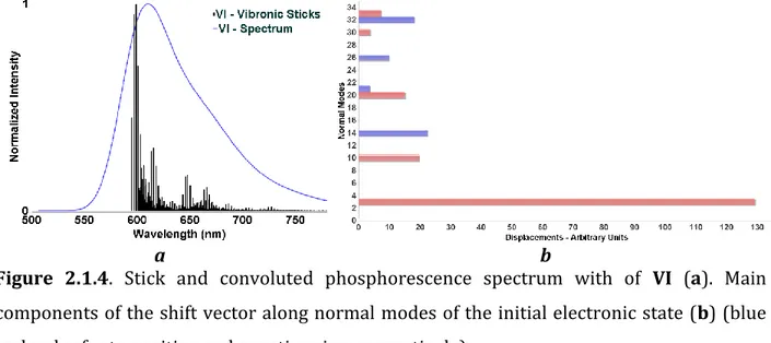
In the case of transition metal complexes, excitation energies from the electronic ground state and equilibrium geometries for excited states were evaluated by means of TD-DFT and unrestricted TD-DFT. One-photon emission (OPE) spectra were also simulated within the Born−Oppenheimer and harmonic approximations by a time independent approach, which effectively takes into account the transitions from the ground vibrational state of the initial electronic state to all the vibrational states of the final electronic state.39 _{Both vertical} (same geometries for both electronic states) and adiabatic (optimized geometry for each electronic state) models were considered together with inclusion (vertical Hessian, VH, or adiabatic Hessian, AH) or not (vertical gradient, VG, or adiabatic shift, AS) of frequency changes and mode mixing between the two electronic states. In all cases, the Franck−Condon approximation was enforced, namely that the transition moment is only marginally affected by (small) geometry modifications. Further details can be found in ref 39_{. For some specific} cases, the lowest normal modes were removed from the vibronic treatment in view of their marginal role in the spectrum and poor description at the harmonic level. Composition and plot of frontier orbitals were determined respectively thanks to the Gaussview and Chemissian packages.40,41

Solvent effects have been modelled using the Polarizable Continuum Model (PCM),42– 44 _{and all the spectra have been generated and managed by the VMS-draw graphical user} interface.45

32

Chapter 1. Accurate Infrared (IR) Spectra for Molecules Containing

the C≡N Moiety by Anharmonic Computations with the Double

Hybrid B2PLYP Density Functional.

Over the past few years, the C=N and C≡N moieties have been deeply investigated,46– 49_{in connection with their intrinsic role as intermediates in reactions involving purines and} proteins.50 _{From another point of view, the simplest form of this compound, HCN, plays a} remarkable role in the interstellar space as a widespread small molecule51–53 _{of relevance for} prebiotic chemistry.54_{Furthermore, cyanocarbons (i.e., organic compounds bearing enough} cyano functional groups to significantly alter their chemical properties) are considered a classical example of discovery-driven research,55 _{tetracyanoethylene (TCNE) and its} derivatives playing a prominent role in the field of magnetic materials.56,57 _{Finally, the} vibration of the cyano group in organic and biological molecules has been studied as an infrared (IR) probe of the local environment in biological systems.58,59_{Several studies have} shown that the CN stretching is highly localized and its frequency is very sensitive to environmental changes.60 _{Therefore, a molecular level understanding of the tuning of} frequency shift, peak width, and intensity change by stereoelectronic and environmental effects is of increasing importance. For this purpose, quantum chemical computations are playing an increasing role toward disentanglement of intrinsic and environmental effects in determining specific spectroscopic signatures.61,62 _{Methods based on density functional} theory (DFT) have been instrumental, especially for infrared and Raman spectra of medium- and large sized molecules, because of their reliability, coupled with favorable scaling with the number of electrons.38,63 _{Several benchmarks have shown that harmonic computations} performed by global hybrid functionals (e.g., B3LYP),22,23_{in conjunction with medium-sized} basis sets and scaled by a reduced number of empirical factors, lead to remarkable agreement with experimental frequencies and intensities of fundamental bands.64,65 _{More recently,} second-order vibrational perturbation theory (VPT2) generalized to include a variational treatment of leading resonances (GVPT2)36,66,67 _{has been shown to deliver accurate} frequencies and intensities for fundamentals, overtones, and combination bands without the need of any scaling factor.37,68,69 _{Unfortunately, global hybrid functionals provide}