PoS(VERTEX 2010)009
Silicon Strip Detectors of the ALICE experiment
Mario Sitta∗
Università del Piemonte Orientale E-mail:[email protected]
Panos Christakoglou1,2
1NIKHEF, Science Park 105, 1098 XG Amsterdam, The Netherlands
2Utrecht University, Faculty of Science, Budapestlaan 6, 3584 CD Utrech, The Netherlands
E-mail:[email protected]
for the ALICE Collaboration
The calibration and performance of the Silicon Drift and Silicon Strip Detectors of the ALICE experiment is presented. In particular the monitoring of the noise, bad channels and drift velocity, the monitoring and quality assurance, along with the charge calibration with cosmic muons and pp collisions are shown.
19th International Workshop on Vertex Detectors - VERTEX 2010 June 06 - 11, 2010
Loch Lomond, Scotland, UK
PoS(VERTEX 2010)009
1. Introduction
ALICE (A Large Ion Collider Experiment) is a general-purpose, heavy-ion detector at the CERN LHC which focuses on QCD, the strong interaction sector of the Standard Model [1]. Its overall dimensions are 16x16x26 m3with a total weight of approximately 10000 t. ALICE consists of a central barrel part, which measures hadrons, electrons, and photons, and a forward muon spectrometer. The central part covers the pseudo-rapidity range of|η| < 0.9 and is embedded in a
large solenoid magnet.
The Inner Tracking System-ITS [2], is the innermost detector of ALICE. The main tasks of the ITS are to localize the primary vertex with a resolution better than 100µm, to reconstruct the secondary vertices from the decays of hyperons and D and B mesons, to track and identify particles with momentum below 200 MeV/c, to improve the momentum and angle resolution for particles reconstructed by the Time-Projection Chamber (TPC) and to reconstruct particles traversing dead regions of the TPC.
The ITS consists of six cylindrical layers of silicon detectors: the Silicon Pixel Detectors (SPD), the Silicon Drift Detectors (SDD) and the Silicon Strip Detectors (SSD). The commission-ing and performance of the two latter systems are the topic of this article.
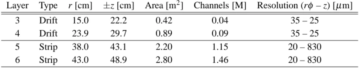
Table 1: Dimensions of the SDD and the SSD.
Layer Type r [cm] ±z [cm] Area [m2] Channels [M] Resolution (rφ – z) [µm]
3 Drift 15.0 22.2 0.42 0.04 35 – 25
4 Drift 23.9 29.7 0.89 0.09 35 – 25
5 Strip 38.0 43.1 2.20 1.15 20 – 830
6 Strip 43.0 48.9 2.80 1.46 20 – 830
The main parameters for both the SDD and the SSD are listed in Table 1. The number, position and segmentation of the layers are optimized for efficient track finding and high impact parameter resolution: in such a way the ITS as a whole allows the precise reconstruction of the trajectories of particles emerging directly from the interaction point. Moreover the four outer layers have analogue readout and therefore can be used for particle identification via dE/dx measurement in the
non-relativistic (1/β2) region. The analogue readout has a dynamic range large enough to provide the
dE/dx measurement for low-momentum, highly ionising particles, down to the lowest momentum
at which tracks can still be reconstructed. The outer layers of the ITS (SSD) are also crucial for the matching of tracks from the TPC to the ITS.
1.1 The Silicon Drift Detectors
The SDD modules are mounted on linear structures called ladders: layer 3 (< r >= 14.9
cm) consists of 14 ladders having 6 modules each, while layer 4 (< r >= 23.8 cm) counts 22
ladders with 8 modules mounted on each one, for a total of 260 modules. Ladders and modules are assembled in such a way to ensure full angular coverage.
One SDD module consists of a drift detector and its front-end electronics. The sensitive area of a detector is split into two drift regions, where electrons move in opposite directions, by a central cathode kept to a nominal voltage of -1800 V. A second bias supply of -40 V keeps the biasing of
PoS(VERTEX 2010)009
the collecting region independent of the drift voltage. Each drift region is equipped with 256 anodes to collect the charges, and three rows of 33 MOS charge injectors used to monitor the drift velocity [3]. The SDD front-end electronics is based on three types of ASICs, two of them assembled on an hybrid circuit which is directly bonded to the sensor, and one located at each end of the ladder, which performs compression and bidimensional two-threshold zero suppression. The sampling rate can be set via software at 20 or 40 MHz.
A cooling system with 52 underpressure demineralized-water circuits is used to take away the power dissipated by the front-end electronics (∼ 6 mW per each PASCAL–AMBRA pair) and to
maintain a temperature stability of< 0.1 K [4]. A dedicated interlock system constantly monitors
pressure and flow to guarantee leak-safety and assure an adequate heat removal. 1.2 The Silicon Strip Detectors
The Silicon Strip Detectors provide a two dimensional measurement of the track position. The system is optimized for low mass in order to minimise multiple scattering. The thickness of the SSD, including support and services, corresponds to 2.2% of a radiation length. Both outer layers
use double sided Silicon Strip Detectors mounted on carbon-fiber support structures, with a strip pitch of 95µm and a stereo angle of 35 mrad. The detection modules consist of one sensor each, connected to two hybrids with six HAL25 chips each [6]. All interconnections between the sensor and the electronics in the detection module are made using aluminum on polyimide cables. The cooling system is optimized in line with the zero heat balance required for all ALICE detectors. The modules are cooled by water running through two thin (40 mm wall thickness) phynox tubes along each ladder. The detector consists of 72 ladders, each one having 22 (34 ladders on layer 5) to 25 (38 ladders on layer 6) modules, resulting into 1698 modules. Each module has 768 P- and 768 N-side strips, making in total more than 2.6 million channels [2, 9].
2. SDD Commissioning results
During the cosmic rays and pp runs 16 out of 260 SDD modules were out of the data ac-quisition, and 4 more modules had one hybrid disconnected, for a total of 92.5% of modules in acquisition. The fraction of good channels in active modules was ≈ 99%. The main source of
excluded channels is one half-ladders switched off due to electrical problems; few other modules are excluded from the acquisition due to either HV or DAQ problems.
The measurement of the anode baseline and of the noise (both raw and corrected for common mode) is provided by pedestal runs, which are special runs performed every ≈ 24 hrs without
zero suppression and without anode-by-anode baseline equalization [5]. Moreover they can tag the noisy anodes, that are then masked during physics runs. The noise is≈ 2.4 ADC units, while the
signal peak is typically≈ 100 ADC counts over the baseline near the anodes, corresponding to a
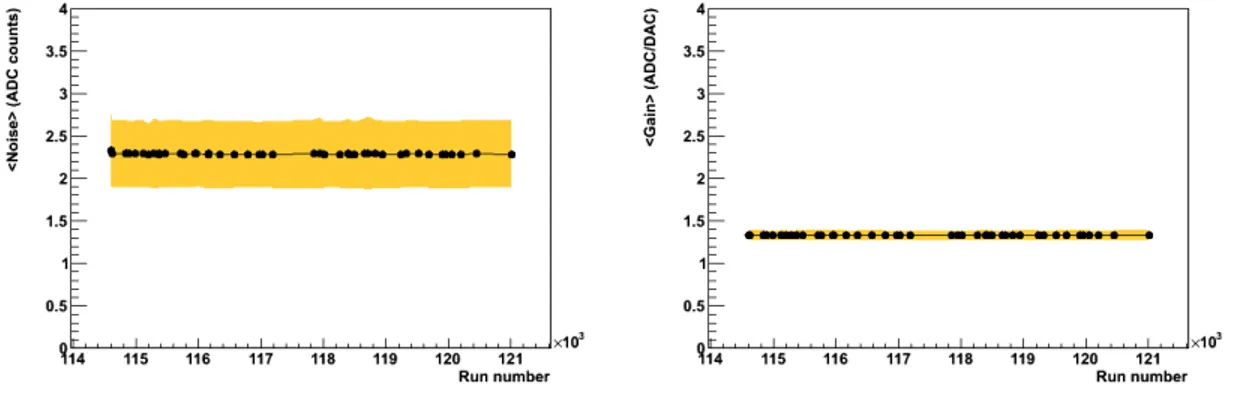
S/N ratio of about 50, and decreases with increasing drift distance. The values of baselines and noise and the fraction of noisy channels (around 0.5%) are all proven to be very stable during the entire data taking period. In Figure 1-left the average value of the noise is shown as a function of the run number for a period of three months.
Pulser runs are special runs without zero suppression and without baseline equalization per-formed every≈ 24 hrs. For each anode a test pulse is sent to the input of the front-end electronics.
PoS(VERTEX 2010)009
Figure 1: The average noise (left) and the average gain (right) for all SDD channels as a function of the run
number from the end of March to the end of May 2010; the yellow band is the RMS of the distribution.
The analysis of a pulser run provides a measurement of the preamplifier gain, and can tag the dead anodes. The gain value and the fraction of dead channels (around 1%) both proved to be very stable during the whole data taking period. In Figure 1 (right) the average gain is shown as a function of the run number for the same time interval as in Figure 1 (left).
2.1 Drift speed
The accurate knowledge of the drift velocity is a crucial element for the precise calibration of a drift detector; to reach a 35 µm resolution a precision of the order of 0.1% is required. For this reason the drift velocity must be very frequently measured and monitored.
Injector runs are special runs with zero suppression and with baseline equalization performed at each LHC fill during the ramp-up phase and used to measure the drift velocity. In these runs the MOS injectors are activated in order to inject charges in known positions. The drift velocity is then extracted from a fit of the measured drift time vs. known drift distance.
The drift speeds, along with the other aforementioned calibration quantities, are stored in the Offline Condition DataBase (OCDB) for the SDD. The reconstruction code can then retrieve this information during the offline reconstruction by automatically selecting the most recent set of calibration data according to the run being analyzed.
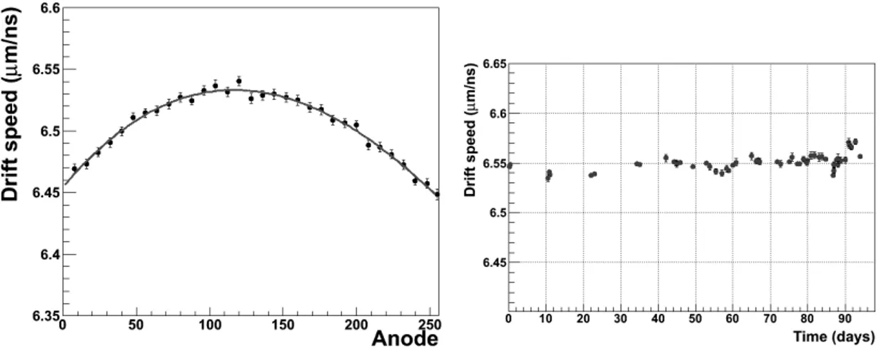
The drift velocity depends on the local temperature as T−2.4, implying that every detector has its own mean drift velocity. Layer 3 has a drift velocity systematically lower than layer 4 because being inner it has slightly higher temperature. Moreover, since heat sources (the voltage dividers) are located at the sensor’s edges, there is also an anode-by-anode dependence of the drift velocity (Figure 2-left). The mean drift velocity is proven to be very stable during the whole data taking period (Figure 2-right). In addition special 1 hour runs were collected in which the average drift velocity was measured every minute; the fluctuations were below 0.15% for most of the modules. 2.2 Time zero
Another parameter calibrated during the commissioning is the time-zero, that is the time offset that has to be subtracted (half-module by half-module) from all measured drift times to obtain the actual particle time. Two strategies have been developed based on simulated data. The first method consists of determining the minimum drift time from the time distribution of all measured
PoS(VERTEX 2010)009
Figure 2: Left panel: Measured SDD drift speed as a function of the anode number for a half sensor; the
shape reflects the location of heat sources near the edges. Right panel: SDD drift speed of one anode during three months of data taking.
clusters. The second method consists of measuring track-to-point residuals and extracting it from the distribution of the residuals in the two detector sides. Differences between the two halves of a ladder are partly due to different cable lengths.
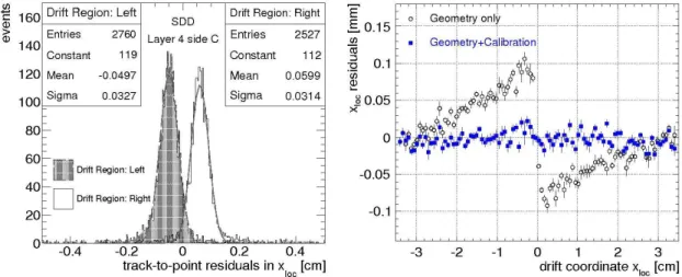
In Figure 3-left an example of the results from the track cluster residuals from cosmic data is shown. Muon tracks in SPD and SSD are fitted using at least five points, and the residuals between the track crossing point taken as reference and the cluster coordinate in SDD are computed. The time offset is extracted by exploiting the opposite sign of the residuals in the two detector sides: an uncalibrated time offset would lead to an over/underestimation of the drift path, and therefore to residuals of opposite signs in the two sides [7]. The time-zero correction has been optimized with the Millepede code, which is used for the geometrical alignment (see [8]) (the other parameters being the degrees of freedom for the rotation and translations of modules, ladders and layers, and the drift speed of those modules with bad MOS injectors, left as a free parameter). The result of this procedure is shown in the right panel of Figure 3: the open points represent the residuals without the time zero calibration, whereas the blue points give the residuals after this correction, both as a function of the drift coordinate.
2.3 Charge calibration
The data sample of muons collected during the 2008 run with cosmic rays (cosmic run in the following) allowed to extract for a subsample of modules the conversion factor from ADC counts to the energy deposited in keV and the dependence of the collected charge on drift time.
Due to the zero suppression applied to the counts in the time bin cells, the diffusion effect can give rise to a dependence of the reconstructed cluster charge on the drift distance: the longer the drift time, the larger the charge diffusion and consequently the larger the fraction of charge in the electron-cloud tails which is more easily cut by the zero-suppression algorithm. This effect is shown in the left panel of Figure 4 where the energy deposit of SDD clusters in two intervals of measured drift time is displayed for a sample of atmospheric muons collected without magnetic field during the 2008 data taking. This effect is accounted for during event reconstruction by
PoS(VERTEX 2010)009
Figure 3: Left panel: Distribution of residuals from tracked cosmic muons for the two sides of the detectors.
Right panel: Residuals as a function of drift coordinate obtained with Millepede with (blue) and without (open points) the time zero calibration.
Energy loss in SDD (A.U.)
0 50 100 150 200 250 Events (A.U.) 0 0.02 0.04 0.06 0.08 0.1 0.12 < 1 µs drift t s µ > 4.5 drift t MPV MPV
Figure 4: Left panel: Distribution of energy deposit (in arbitrary units) for clusters reconstructed in the SDD
detector for two intervals of drift time. Fits with a convolution of a Landau and a Gaussian are superimposed. Right panel: Charge distribution for each of the SSD modules.
applying to the reconstructed cluster charge a linear correction, extracted from detailed simulations of the detector response and checked with the cosmic and first pp data. The shape of the energy deposit distribution is well reproduced by a Landau function convoluted with a Gaussian; the peak of the distribution is located at a lower value of energy for particles with large drift times.
Figure 4-left shows the charge distribution collected from each SDD module: for more than 85% of the modules the dE/dx distributions have the MPV within 5% from the expected value.
Special corrections are needed only for 15 modules with lower charge collection efficiency, all of them connected to known hardware problems or non-standard applied voltage.
PoS(VERTEX 2010)009
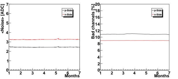
<Noise> [ADC] 0 1 2 3 4 5 6 7 p-Side n-Side Months 1 2 3 4 5 6 7 Bad channels [%] 0 2 4 6 8 10 12 14 16 18 20 p-Side n-Side Months 1 2 3 4 5 6 7Figure 5: The time evolution of the average noise (left plot) and the percentage of bad channels (right plot)
for both sides of the SSD.
3. SSD Commissioning results
During the 2009/2010 runs 1557 out of 1698 SSD modules, i.e.≈ 92%, were active. The main
source of excluded channels are 6 half-ladders that are switched off due to electrical problems. The resulting signal over noise ratio was S/N > 40. The noise values for each channel as well as the
number of dead or noisy channels are provided by the Detector Algorithm (DA) which runs online. The extracted objects are transferred to the Offline Conditions Data Base (OCDB) and then used during the reconstruction. The average noise as a function of time for both the P- and N-side strips is shown on the left plot of Figure 5. The values, stable over a period of several months, are≈ 2.4
and≈ 3.5 ADC units for the P- and N- side, respectively. The time evolution of the percentage of
bad channels is also shown in Figure 5-right. The values for both sides are mainly dominated by the six switched off half-ladders (electrical connection problems) and the corresponding masked channels. The latter group is masked either by the DA or manually, with the reason being the high noise they exhibit.
3.1 Geometrical alignment
The geometrical alignment of both systems starts from the measurements taken during the assembling phase by surveying the positions of the modules on the ladders and the measurement of the positions of the ladder end points on the support cone.
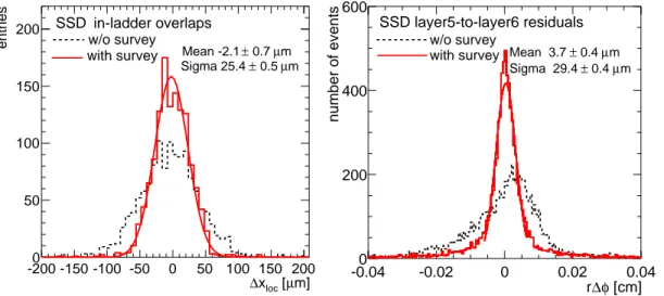
The SSD modules are mounted with a small overlap for both the longitudinal (z, modules on the same ladder) and transverse directions (rφ, adjacent ladders). These overlaps allow us to verify the relative position of neighbouring modules using double points produced by the same particle on the two modules. Figure 6-left shows the∆xloc, defined as the distance in the local x direction
on the module plane between the position of one point on the first module and the projection of the point of the second module on the plane of the first, with and without the survey corrections, for both SSD layers. The clear improvement is evident, resulting in a spread ofσ ≈ 25.4µm. Taking also into account that this value is the result of the combined spread of the two points, one obtains
PoS(VERTEX 2010)009
m] µ [ loc x ∆ -200 -150 -100 -50 0 50 100 150 200 entries 0 50 100 150 200 SSD in-ladder overlaps w/o surveywith survey Mean -2.1 ± 0.7 µm
m µ 0.5 ± Sigma 25.4 [cm] φ ∆ r -0.04 -0.02 0 0.02 0.04 number of events 0 200 400 600 m µ 0.4 ± Sigma 29.4 m µ 0.4 ± Mean 3.7 w/o survey with survey SSD layer5-to-layer6 residuals
Figure 6: Left: The distribution of∆xloc, the distance between two points in the module overlap regions
along z on the same ladder. Right: The distribution of the rφresiduals between straight-line tracks defined from two points on layer 6 and the corresponding points on layer 5.
a value of≈ 18µm for the position resolution for a single point. This value is compatible with the expected intrinsic spatial resolution of about 20µm (see Table 1). This indicates that the residual misalignment after applying the survey is negligible with respect to the intrinsic spatial resolution [7].
Figure 6-right shows the distribution of the rφ residuals between tracks through layer 6 and points on layer 5. This was performed by using the two points of the outer SSD layer to define a straight track (cosmic runs with no magnetic field) and calculate the corresponding residuals with respect to the points on layer 5. The spread of the distribution after applying the correction coming from the survey data isσ ≈ 29.4µm. This value contains a contribution from the uncertainty in the track trajectory due to the uncertainties in the points on the outer layer. Assuming the same resolution on the outer and inner layers and taking into account the geometry of the detector, the effective single point resolution spread is 21µm, compatible with the value obtained with the pre-vious method. The same exercise was repeated for the z coordinate, with the result being consistent with the effective single point intrinsic resolution of 800µm. This again indicates that the residual misalignment in z is much smaller than the intrinsic SSD resolution [7].
3.2 Time alignment
Each HAL25 SSD chip, connecting 128 input channels, consists of a pre-amplifier, a shaper and a capacitor to store the voltage signal proportional to the collected charge on a strip of the sensor. The shaping time is remotely adjustable via JTAG protocol between 1.4 and 2.1µs and the analogue signals are stored in a sample-hold circuit, controlled by an external HOLD signal. This HOLD signal is derived from the L0 trigger signal, adequately delayed to match the shaping time of the HAL25. The delay between the arrival of the physics event and the HOLD signal activation, called L0 delay, depends on several different delay sources: the HAL25 shaping time; the length of the cables driving the signals from the trigger detectors to the Central Trigger Processor (CTP),
PoS(VERTEX 2010)009
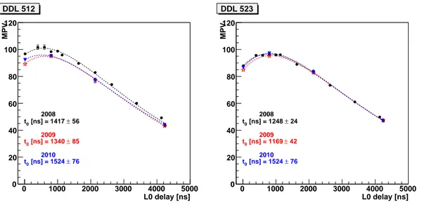
L0 delay [ns] 0 1000 2000 3000 4000 5000 MPV 0 20 40 60 80 100 120 2008 56 ± [ns] = 1417 0 t 2009 85 ± [ns] = 1340 0 t 2010 76 ± [ns] = 1524 0 t DDL 512 L0 delay [ns] 0 1000 2000 3000 4000 5000 MPV 0 20 40 60 80 100 120 2008 24 ± [ns] = 1248 0 t 2009 42 ± [ns] = 1169 0 t 2010 76 ± [ns] = 1524 0 t DDL 523Figure 7: The MPV extracted from the Landau fits for the 2008, 2009 and 2010 runs as a function of the
selected L0 delay in ns (see text for details).
from the CTP to the sub-detector interface (Local Trigger Unit–LTU), to the Front-End ReadOut Modules (FEROM) and finally to the endcaps; the internal delay of the CTP logic and the front-end electronics. Due to the fact that most of these quantities are unknown, the total L0 delay has to be measured directly.
For this study, we relied on cosmic triggers without the presence of the magnetic field. The relevant runs were taken in 2008 and 2009 (in 2009 after the mini-frame upgrade); the measure was repeated also in 2010. The read-out partition included all the ITS sub-detectors. The trigger was provided by the SPD FastOR [10]. For each run, the programmable delay time was changed accordingly. The offline analysis was performed for all the reconstructed clusters grouped by
De-tector Data Link–DDL. The results of the L0 delay scan were fitted for each DDL with a function
of the type of the one in Eq. 3.1:
f(t) = A0
t− t0
τ e−( t−t0
τ ) (3.1)
where A0is the amplitude of the signal, t0is the L0 arrival time andτis the shaping time.
Figure 7 shows the Most Probable Value–MPV extracted from the Landau fit for each run, as a function of the selected L0 delay in ns, for two DDLs: DDL–512 (A–side) and DDL–523 (C–side). The black points correspond to the 2008 measurements, whereas the red and blue ones to the 2009 and 2010 ones, respectively. The dashed curves are the fits with the fitting function shown in Eq. 3.1. The agreement between the data points of all the periods for the C–side DDL is clearly seen. On the other hand, this is not the case for the A–side, where the 2009 and 2010 points (consistent between them) are slightly but systematically below the 2008 ones. This decrease is quantified to be of the order of≈ 6.5% and it is mainly attributed to the mini-frame modifications that took place
PoS(VERTEX 2010)009
SSD module number
0 200 400 600 800 1000 1200 1400 1600
Charge [arb. units]
0 50 100 150 200 250 300 1 10 2 10 = 7 TeV s pp @
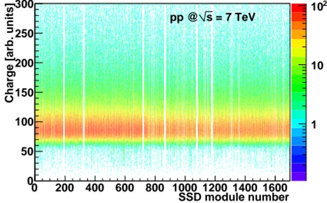
Figure 8: The charge distribution for each of the SSD modules.
3.3 Gain calibration
The gain calibration of the SSD has two components: relative calibration of the P and N sides and conversion factor of ADC values to energy loss. The first pass of the calibration constants was already determined in the laboratory, using cosmics on a spare ladder with a data-acquisition system setup which matches the one used in the experiment. These constants were refined first during the cosmic runs with the pixel trigger [9], and then determined with better precision during the first LHC runs in 2009/2010. This allowed the extraction of the gain factor for each side of each SSD module.
In addition, detailed studies were performed to check the calibration constants at the chip level. Preliminary results show that the calibration at the chip level improves the stability of the P- and N-side gains by 10%.
Figure 8-right shows the charge distribution collected from each SSD module. The switched off half-ladders along with the masked modules are clearly seen. The MPV values are fairly con-stant for all the modules included in the readout and demonstrate a remarkable stability with time.
4. Performance
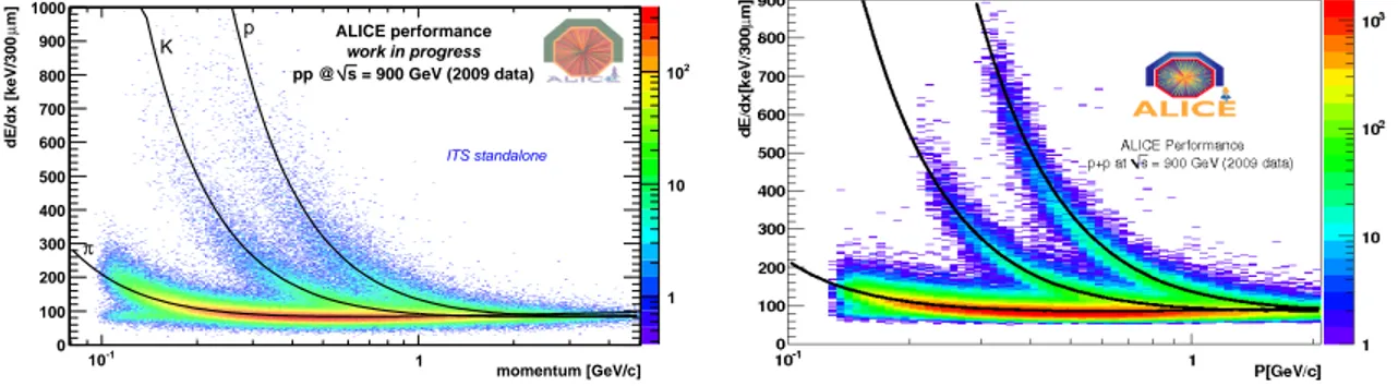
The truncated mean of the four dE/dx samples obtained for each track, reconstructed with
the ITS standalone tracking, from SDD and SSD detectors is shown in the left panel of Figure 9 as a function of particle momentum. The superimposed theoretical energy loss for protons, kaons and pions is also plotted, showing a remarkable agreement. In the right panel of this Figure the same quantity is shown for all tracks reconstructed by the TPC and the ITS working together. The standalone ITS tracking allows particle identification to be extended to lower momentum values but with a smaller separation betweenπ, K and p due to a worse momentum resolution. The latter is of the order of 13% which is close to the design value [1].
5. Summary
During the 2009-2010 cosmic ray and pp runs more than 90% of the SDD and SSD channels were included in the acquisition. The collected data were used to commission both systems and start the procedure for the geometrical alignment, for each detector separately and for the ITS as
PoS(VERTEX 2010)009
momentum [GeV/c] -1 10 1 m] µ dE/dx [keV/300 0 100 200 300 400 500 600 700 800 900 1000 1 10 2 10 ALICE performance work in progress = 900 GeV (2009 data) s pp @ p K π ITS standaloneFigure 9: Truncated mean of the energy deposition as a function of particle momentum obtained from SDD
and SSD detectors for all tracks reconstructed by the ITS standalone (left) and ITS+TPC tracking (right) (ALICE performance, work in progress).
a whole. Frequent calibration runs were taken to properly monitor noise, pedestals, bad channels, gains and the SDD drift velocity. All monitored parameters are proven to be very stable over the entire period. The ALICE Silicon Drift and Silicon Strip Detectors turned out to be well understood and fully under control, and they are ready for the ongoing pp data taking and the forthcoming PbPb collisions. They already gave an important contribution to the tracking and particle identification in different analyses of the 900 GeV pp data, and will contribute also to the future analyses of the pp and lead-lead data.
References
[1] K. Aamodt et al. [ALICE Collaboration], J. Phys. G30, (2004) 1517; K. Aamodt et al. [ALICE Collaboration], J. Phys. G32, (2006) 1295. [2] K. Aamodt et al. [ALICE Collaboration], JINST 3, (2008) S08002.
[3] A. Rashevsky et al., Charge injectors of ALICE Silicon Drift Detector, Nucl. Instrum. Meth. A572 (2007) 125.
[4] S. Coli et al., The cooling system of the Silicon Drift Layers of the ALICE Inner Tracking System, ALICE Internal Note ALICE–INT–2008–008
[5] B.Alessandro et al., Operation and calibration of the Silicon Drift Detectors of the ALICE experiment during the 2008 cosmic ray data taking period, JINST 5 (2010) P04004
[6] C. Hu-Guo et al., “The HAL25 front-end chip for the ALICE silicon strip detectors”, Proceedings of the 7th Workshop on Electronics for LHC Experiments, Stockholm, Sweden (2001),
http://cdsweb.cern.ch/record/528581;
C. Colledani, C. Hu and J.D. Berst, HAL25 V3 user manual v0:1, LEPSI-IN2P3-CNRS/ULP, Strasbourg France.
[7] K. Aamodt et al. [ALICE Collaboration], JINST 5 (2010) P03003
[8] A. Rossi, Alice Alignment Tracking and Physics Performance Results, this Proceedings [9] P. Christakoglou et al. [ALICE Collaboration], PoS (EPS-HEP 2009) 124.