Spin Coherence Time studies for the storage ring EDM search

(1)

Universit`

a degli Studi di Ferrara

DOTTORATO DI RICERCA IN FISICA, XXV ciclo Coordinatore Prof. Vincenzo Guidi

Spin Coherence Time studies

for the storage ring

EDM search

Dottoranda: Guidoboni Greta

Relatore: Dott. Lenisa Paolo

(2)

(3)

Introduction

The present work has been developed within the framework of the project to measure the Electric Dipole Moment (EDM) of charged particles in a storage ring. The measurements presented here were made at the COSY (COoler SYnchrotron) ring located at the Forschungszentrum-J¨ulich GmbH (Germany).

The measurement of a non-zero EDM aligned with the spin of fundamen-tal particles would contribute to solving one of the puzzles of contemporary physics, the so-called baryon asymmetry, that asks why matter dominates over anti-matter in our universe. According to the Big Bang Theory, at the origin of the universe an equal amount of matter and anti-matter was present. This symmetry must have been broken by mechanisms violating charge symmetry C and the combined charge-parity symmetry CP under conditions far from thermal equilibrium (see Sakharov’s criteria). Despite the fact that the Standard Model contains all these elements, it is not able to explain the size of the current baryon asymmetry, especially because the amount of CP violation (essentially coming from the weak sector) is too small. This CP violation is scaled to match the observed cross sections in the decay of K-meson and B-meson. What is needed is a window that would allow us to observe new forms of CP violation. One way to proceed

(6)

is to measure the time-reversal violation determined by the size of an EDM aligned with the spin of a particle, nucleon, or atomic system.

The EDM is a charge displacement that lies along the particle’s spin axis. Under a parity transformation P which inverts the spacial coordinates, the spin direction remains unchaged while the EDM flips. Under a time reversal operation T which inverts the time coordinate, the EDM stays the same and the spin direction is inverted. The failure of either transformation to reproduce the original system indicates that the presence of an EDM along the particle’s axis represents a violation of both parity and time-reversal symmetries. Assuming the conservation of the combined symmetries CP T , a violation of T represents a violation of CP . Thus time reversal violation experiments represent a way to look for CP violation aside from comparing particle and anti-particle reaction rates.

The theoretical predictions based on multi-loop Standard Model me-chanisms (e.g. neutron | ⃗dn| ∼ 10−34 e·cm) are several orders of magnitude

below the current EDM experimental limits (| ⃗dn| ∼ 10−26e·cm). In contrast,

models beyond the Standard Model forsee EDMs well within the planned experimental precision. The measurement of a non-vanishing EDM at the sensitivity of present or planned experiments would clearly prove the exi-stence of new CP violating meachanisms beyond the Standard Model.

Noting that the first CP non-invariance was observed in K-meson decay in 1964, the question of the symmetry properties of fundamental forces or particles was put forward by Purcell and Ramsey in 1951. They searched unsuccessfully for a parity-violating up-down asymmetry in the scattering of neutrons from nuclei. Even if they were not explicity looking for an EDM, their work is usually recalled as the first EDM experiment. After

(7)

Introduction V that, the EDM search intensified and the level of experimental precision has improved steadily ever since, now including heavy atoms and molecules as well as neutrons. For a neutral system, the usual method for detecting the EDM ⃗d is to apply an electric field ⃗E and look for the energy shift

⃗

d · ⃗E. Unfortunately, this method cannot be used for charged particles which would be accelerated by the electric field and then lost.

The development of storage ring technology and polarized beams made possible the recent proposal to measure the EDM of charged particles. The proposed solution is the use of a storage ring where the polarized charged particle beam can be kept circulating while interacting with the radial elec-tric field always present in the particle frame. Starting with a longitudinally polarized beam (particle spins aligned along the velocity), the EDM signal would be detected as a polarization precession starting from the horizontal plane and rotating toward the vertical direction.

There are two fundamental conditions to fulfill in order to realize this experiment. One is freezing the polarization precession frequency in the horizontal plane to the revolution frequency of the beam in the ring, so that the beam will be always longitudinally polarized. The second condition is to guarantee a long horizontal polarization lifetime which defines the observation time available to measure the EDM signal.

A deep comprehension of beam and spin dynamics in a storage ring is needed to study the feasibility of the proposed EDM experiment for charged particles. In particular, the understanding of spin dynamics is a crucial point in order to provide a long horizontal polarization lifetime. The sta-ble spin axis in a storage ring is along the vertical axis, orthogonal to the ring plane. Thus, as soon as a spin moves out from the stable direction,

(8)

it will start precessing around it with a frequency proportional to the rel-ativistic factor γ of its motion and the local magnetic field. The number of spin precessions per turn around a storage ring is called the spin tune. Since particles have slightly different velocities, the spins will precess with different frequencies, spreading around in the horizontal plane and making the horizontal polarization shrink and vanish. The horizontal polarization lifetime represents the obervation time available to detect the EDM signal and is called the spin coherence time. The goal for the deuteron EDM ex-periment is to achieve an EDM sensitivity of 10−29 e·cm, which requires a spin coherence time of at least 1000 s along with the ability to measure microradians of polarization rotation.

The aim of this work is the analysis of the mechanisms which control the spin coherence time in a storage ring as a part of the feasibility studies for the deuteron EDM experiment. For this reason a series of dedicated studies has been started at the COSY ring in J¨ulich. The COSY ring provides beams of polarized protons and deuterons in a momentum range from 300 MeV/c to 3.7 GeV/c. Beam polarimetry tools are also available, such as the LEP (Low Energy Polarimeter) to measure the polarization of the states injected and the EDDA scintillator detectors used as a mock EDM polarimeter.

A first set of measurements was devoted to study the spin coherence time in presence of a radio-frequency (rf) solenoid induced spin resonance. Since the width of this resonance depends on the spin tune spread and thus on the particle momentum distribution, it represents a good starting point to estimate the size of the spin tune spread before moving to a direct measurement of the spin coherence time. A vertically polarized deuteron beam was injected in COSY and accelerated to a momentum of 0.97 GeV/c.

(9)

Introduction VII A continuous polarization measurement was provided by slowly extracting the beam into a thick carbon target and detecting the elastically scattered deuterons in the EDDA polarimeter. The use of electron-cooled and un-cooled beams permitted observation of the effect of momentum spread and beam size on the polarization while running the rf-solenoid either at fixed or variable frequency. In order to analyze the data, I developed a “no lattice” model together with Dr. E. J. Stephenson, based on two matrices to decribe the spin precession about the vertical axis and the spin rotation due to the solenoid effect.

The second experiment was devoted to the measurement of the horizon-tal polarization lifetime as a function of time. It required the development of a dedicated data acquisition system aimed at detecting the precession of the horizontal polarization as a function of time. Data were analyzed using a set of template curves which allowed the study the contribution of beam emittance (transverse beam size) to the spin coherence time. Then, it was succesfully verifed the possibility to correct emittance effects on the spin tune spread using sextupole magnets, obtaining a longer spin coherence time.

The thesis is divided in six chapaters:

• Chapter 1 yields a theoretical overview of the EDM as probe of new physics including the experimental results achieved up to now. The new method for the measurement of a charged particle EDM in a storage ring closes the chapter.

• Chapter 2 provides the basic elements of beam dynamics in a storage ring which are necessary to understand the analysis and the

(10)

measure-ments presented in the thesis.

• Chapter 3 describes the COSY storage ring where the experiments have been conducted. It contains the definition of polarization for a spin-1 particle such as the deuteron and the methods to measure it. • Chapter 4 illustrates the first set of measurements which focus on the

effects of synchrotron oscillations on the vertical polarization and the “no lattice model” used for the analysis.

• Chapter 5 shows the direct measurement of horizontal polarization as a function time including the emittance effects and the sextupole corrections to the depolarization with time.

• Chapter 6 contains a summary describing what has been achieved and the prospects for future developments.

(11)

Chapter 1 The Electric Dipole Moment as

a probe of CP violation

1.1 Baryon asymmetry

In cosmology, an important fact still lacking explanation is the existence of the large amount of matter which forms the galaxies, the stars and the interstellar medium. There is essentially no antimatter in a universe that started with no particle content right after inflation. This chapter will explore how this problem of baryogenesis is linked to the possible existence of an electric dipole moment (EDM) aligned along the spin axis of particles. All explanations of baryogenesis in the early universe necessarily require a significant amount of CP violation, the combination of charge conjugation and parity symmetries, that is a characteristic of an EDM.

The matter content of the universe usually is quantified by the ratio of the number density of baryons nb to the number density of photons nγ, also

called the asymmetry parameter, which is:

η = nb/nγ = (6.08 ± 0.14) × 10−10 (1.1)

as the derived from the CMB saltellite data and from primordial nucleosyn-thesis data [1]. At the present temperature T = 2.728 ± 0.004 K of the universe, the photon number density is nγ = 405 cm−3. There is strong

evidence that the universe consists entirely of matter, as opposed to anti-matter, and the few antiprotons np¯/np ∼ 10−4 seen in cosmic rays can be

explained by secondary pair production processes.

The predicted number of baryons and antibaryons is minuscule, nb/nγ =

(12)

n¯_b/nγ ∼ 10−18, which for baryons is more than 8 orders of magnitude below

the observed value (see Eq. 1.1). The process responsible for this unexpect-edly large baryon asymmetry of the universe, generated from an initially symmetric configuration, is called baryogenesis.

The general criteria which allow for the dynamical generation of a baryon asymmetry from an initial baryo-symmetric configuration were formulated by Sakharov in 1967 [2] and they include:

1. Violation of baryon number B . The baryon number is defined as B = nb− n¯_b. There must be elementary processes that violate baryon

number such that baryogenesis can proceed from an initial B = 0 to a universe with B > 0.

2. Violation of C and CP symmetries. It is demonstrated that if the charge conjugation symmetry C and the combined symmetry CP were exact, then the reactions that generate an excess of baryons would occur at the same rate as the conjugate reactions that generate an excess of antibaryons. Thus, the baryon asymmetry would retain its initial value η = 0.

3. Departure from thermal equilibrium. Baryon asymmetry gen-erating processes must take place far from thermal equilibrium. If this was not the case, particle production reactions and their inverses would have the same rate and there would be no net increase in the number of particles.

Remarkably, over the years it was realized that the Standard Model (SM ) does contain all three ingredients. Despite that, the predicted baryon asymmetry falls orders of magnitude short of the baryon asymmetry that is observed experimentally. In particular, the SM contributions to CP violation are too small to explain baryogenesis.

1.2 CP violation in the SM and beyond

In the standard model, treating neutrinos as massless, there are two sources of CP violation: one is the phase δ in the quark mixing matrix and the other is the θQCD coefficient.

The discovery and exploration of CP violation in the neutral B meson system [3] is, along with the existing data from CP violation observed with

(13)

1.2 CP violation in the SM and beyond 3 K-mesons [4], in accord with the minimal model of CP violation known as the Kobayashi-Maskawa (KM) mechanism. This introduces the 3 × 3 unitary matrix V for three quark families (called the CKM mixing matrix) which defines the strength of flavor changing weak decays. Indeed, |Vij|2 is

the probability that a quark of i flavor decays into a quark of j flavor. V involves three mixing angles and one CP violating phase δ. The smallness of CP violation is not because δ is small. This phase can be large, but the observed effects are strongly suppressed by small mixing angles. While the CKM matrix allows for CP violation in the quark-W boson coupling, it does not explain all of the observed CP asymmetry needed for baryogenesis. That is, the level of observed asymmetry between matter and antimatter in the universe is not explained by the Standard Model.

In quantum chromodynamics (QCD), CP violation comes from the so-called θ term, an additional gauge kinetic term of the Lagrangian. If its coefficient θQCD is nonzero, the violation of both P and T (or CP assuming

the CP T theorem) symmetries occurs. Moreover, if θQCD were O(1), one

would predict a neutron EDM of sufficient size to ensure that the first EDM experiment of Purcell and Ramsey [5] would have detected it. In fact θQCD

is now known to be tuned to zero, or at least to cancel, to better than one part in 1010. This tuning is the well known strong CP problem of the Standard Model. In other words the strong interactions preserve CP to high degree of precision. It is not known wether θQCD is small due to

an accidental cancellation or to some dynamical mechanisms. The most popular explanation is the existence of a new symmetry of QCD, called Peccei-Quinn symmetry [6], such that θQCD becomes a dynamical variable.

The spontaneous breaking of the symmetry leads to a very light boson called the axion.

The standard model is not a complete theory [7] because it does not ex-plain the particle-antiparticle asymmetry in the universe nor solve the hier-archy problem - why the masses of the known particles are so much smaller than the fundamental Plank mass (1019 GeV/c) or the grand-unification mass (1016 _{GeV/c). And it does not incorporate gravity. One of the most}

plausible extensions of the standard model is SuperSymmetry (SUSY), a symmetry between bosons and fermions. It adds new sources of CP viola-tion but it doubles the number of particles. Each particle of the standard model has a more massive superpartner, so for example the photon’s super-partner is the photino and the electron’s is the selectron. Spin-zero bosons like the selectron can engage in CP violating interactions with electrons and quarks. Since the new interactions introduced by SUSY can provide a measurable electric dipole moment of fundamental particles, the EDM can

(14)

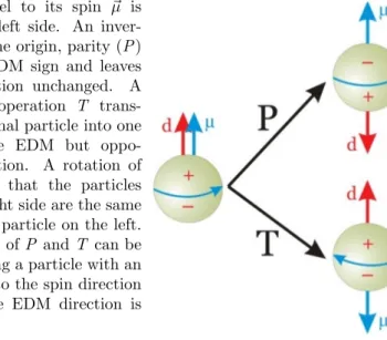
Figure 1.1: A particle with an EDM ⃗d parallel to its spin ⃗µ is shown on the left side. An inver-sion through the origin, parity (P ) reverses the EDM sign and leaves

the spin direction unchanged. A

time reversal operation T trans-forms the original particle into one with the same EDM but oppo-site spin direction. A rotation of 180◦ illustates that the particles depicted on right side are the same and unlike the particle on the left. Thus, violation of P and T can be seen as changing a particle with an EDM parallel to the spin direction into one whose EDM direction is antiparallel.

be a probe of new physics, as is explained in the following section.

1.3 The EDM as probe of new physics

As mentioned in the previous sections, time reversal and CP violation are closely related, in the sense that any CP T invariant interaction that violates one must violate the other. Nevertheless, CP and T are different symmetries with different physical consequences, so possible T violating observables open a new window on standard model tests and new physics searches. In particular, the effects of true CP violation are essentially lim-ited to flavor changing processes such as K and B decays, while T odd observables such as electric dipole moment are also relevant for flavor diag-onal channels.

The EDM of a fundamental particle is a charge displacement within the particle volume. It necessarily lies along its spin axis, because all compo-nents perpendicular to that average to zero. The alignment of spin and the EDM leads to violation of time reversal T, that inverts the time coordinate t → −t, and parity P, that inverts the spatial coordinates ⃗r → −⃗r. As shown in Fig. 1.1, reversing time would reverse the spin direction but leave the EDM direction unchanged. So the existence of an EDM would be a vi-olation of T. A parity operation would leave particle’s spin unchanged but reverse the EDM sign, violating the P symmetry. Assuming the validity of the CPT theorem, violation of T implies a violaton of CP symmetry.

(15)

1.3 The EDM as probe of new physics 5 The idea to use the electric dipole moments of particles as a high-precision probe of symmetry properties of the strong interactions is due to Purcell and Ramsey in 1951. Remarkably, it precedes not only the dis-covery of CP violation in K mesons but also the disdis-covery of parity violation in weak interactions. It was only 25 years later that the establishment of QCD as the theory of strong interactions led to the possibility of P and CP violation by the θ term. Although EDMs are not the only observables sensitive to non-CKM sources of CP violation, the remarkable degree of precision to which they can currently be measured endows them with a privileged status.

1.3.1 Theoretical predictions

The predicted EDM effects due to CKM mixing in the standard model are extremely small. The quark EDMs are only generated at the three-loop level and are expected to be [10]:

dCKM_q ≃ 10−34e cm (1.2) while the electron EDM only receives contributions from four-loop diagrams (at least for massless neutrinos) and should be:

dCKM_e ≤ 10−38e cm. (1.3) The contributions to the neutron and proton EDM from the θQCD term in

the QCD lagrangian is [11]: |dθ n| = |d θ p| ≃ 4.5 × 10 −15 θQCD (1.4)

while the deuteron EDM is expected to be zero. In fact, the upper limit on dn (see Sec. 1.3.2) now sets the upper limit on θQCD at ≤ 10−11.

Another scenario comes from SUSY where there are two contributions to CP violation: one from the quark-EDM (dup and ddown) and the other

from the chromo-EDM (dc

up and dcdown) where the EDM is generated in a

loop containing a supersymmetric particle. Defining ∆ = ddown− dup/4, ∆+= dcup+ dcdown, ∆

−

= dc_up− dc down,

neutron, proton and deuteron EDMs [12] are given by:

dn = 1.4∆ + 0.83∆+− 0.27∆− (1.5)

dp = 1.4∆ + 0.83∆++ 0.27∆− (1.6)

(16)

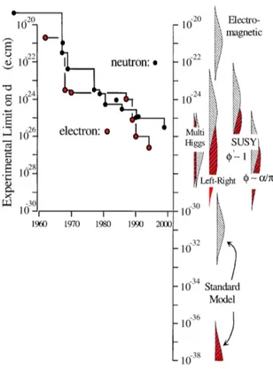
Figure 1.2: The experimental limits reached for neutron (black) and electron (red) EDMs are shown on the left side. On the right side there are the theoretical predictions of the standard model (the smallest values) and beyond, such as Multi Higgs, Left-Right, and SUSY

mod-els. Although no EDM has been

measured yet, a discovery of a non-zero EDM between the current ex-perimental bounds and the stan-dard model calculations would be a signal of new physics [8].

If a non-zero deuteron EDM is measured, it would have a special sensitivity to the chromo-EDM due to the large coefficient of ∆− in Eq. 1.7.

Because the SM contributions are expected to be small, EDMs are an excellent place to search for the effects of new physics. In Fig. 1.2 a com-parison between experimental limits and the wide scenarios of theoretical expectations from the SM and beyond are shown.

No EDM of a fundamental particle has been measured yet. But if a non-zero EDM value is found between the actual experimental limits and standard model predictons it will be a clear signal of new physics and thus it will point to a new CP violation source.

1.3.2 Experiments

After the first experiment in 1951, the EDM search intensified and the level of experimental precision has improved steadily ever since. Indeed, following significant progress throughout the past decade, the EDMs of the neutron and several heavy atoms and molecules have been found to vanish to remarkably high precision.

(17)

1.3 The EDM as probe of new physics 7 In these measurements, the basic idea for detecting an EDM is to apply an electric field and look for the energy shift − ⃗d · ⃗E. In most of the EDM experiments there is an external magnetic field ⃗B parallel to ⃗E. Considering a particle of spin 1/2, the energy difference between magnetic and electric fields parallel or antiparallel is given by:

hν = 2µB ± 2dE, (1.8) where h is Plank’s constant, ν is the spin precession frequency, µ is the magnetic dipole moment and the ambiguous sign is determined by whether d and µ are parallel or antiparallel to each other. The tiny EDM effect is extracted by switching the polarity on the plates generating the electric field, thus reversing the sign of ⃗E relative to ⃗B. Subtracting the measured frequencies cancels out the magnetic term and the EDM is given by:

d = h∆ν

4E (1.9)

Some results in the last decade are:

• |de| ≤ 1.6 × 10−27e · cm, the electron EDM limit derived from205T l, a

paramagnetic atom [13].

• |dn|exp ≤ 2.9 × 10−26e · cm, the neutron EDM limit measured on ultra

cold neutrons [14].

• |datom|exp ≤ 3.1 × 10−29e · cm, the atomic EDM limit measured on 199

Hg, a diamagnetic atoms from which an upper limit on the proton EDM has been derived (|dp| ≤ 7.9 × 10−25e · cm) [15].

The atomic EDMs are complementary to those of the electron and neu-tron because they receive contributions not only from the EDMs of their constituents but also from CP violating eN or πN interactions (where N stands for a nucleon). Future experiments may improve the sensitivity sig-nificantly, by as much as four orders of magntude for de.

There are also prospects for new or greatly improved sensitivities to other EDMs, such as the muon, proton and deuteron. In these cases, the basic idea described for neutral systems does not work, since charged particles would be lost in an electric field. A new technique has to be developed and a plausible solution is a storage ring. For example, a proton or deuteron beam can be kept circulating in a storage ring with the polarization aligned along the momentum. The EDM signal would then arise from the interaction

(18)

of the spin particles with a radial electric field (see Sec. 1.4). A proposal for the proton EDM experiment has been submitted with a sensitivity of 10−29e cm. To roughly estimate the scale of new physics probed by p/d EDM experiments, the EDM can be expressed on dimensional grounds as:

di ≈

mi

Λ2e sin φ (1.10)

where mi is the quark or lepton mass, sin φ is the result of CP violating

phases, and Λ is the new physics mass or energy scale. For mq ∼ 10 MeV

and sin φ of order 1/2, one finds

|dp| ∼ |dd| ∼ 10−24

 1TeV Λ

2

e cm (1.11)

Thus, for a dp or dd ∼ 10−29e cm the sensitivity probe would be Λ ∼ 300

TeV, a scale which is well beyond the center of mass energy of the LHC. Considering SUSY with superpartner masses MSU SY ≤ 1 TeV, if a dp or

dD ∼ 10−29e cm were not observed, sin φ would be very small, ≤ 10−5.

No EDM has been found, but the current experiments set important constraints on the theoretical models. It is critical to carry out EDM ex-periments on different particles in order to understand where the source of CP violation originates.

1.4 EDM search in storage rings

As mentioned in the previous section, the new proposal to measure the EDM of a charged particle is based on the employment of a storage ring, a type of accelerator in which a particle beam can be kept circulating for a long period, up to hours.

Detection methods rest mainly on observing the precession of the polari-zation in an external electric field. Beginning with a longitudinally polarized beam in the storage ring, the EDM can be detected as a rotation of the pola-rization from the longitudinal to the vertical direction due to the interaction with the inward radial electric field that is always present in the particle frame (see Fig. 1.3(a)). This field, which bends the particle trajectories into a closed orbit, is present whether the ring is magnetic or electrostatic (as has been proposed for the proton case). However, it is first necessary to arrange the ring fields so that the precession of the spin relative to the velocity in the ring plane is suppressed. That precession (without the EDM

(19)

1.4 EDM search in storage rings 9 component) is given by the Thomas-BMT equation [16] :

⃗ ωG= ⃗ωS− ⃗ωC = − q m  G ⃗B −  G − m p 2 ⃗ β × ⃗E c  (1.12)

where it is assumed that ⃗β · ⃗B = ⃗β · ⃗E = 0, and ⃗ωS is the spin precession in

the horizontal plane, ⃗ωC is the particle angular frequency and G = (g − 2)/2

is the particle anomalous magnetic moment (also denoted by a for leptonic anomalous moments). The spin precession can be frozen against the particle velocity with different methods, depending on the sign of the anomalous magnetic moment.

(a) (b)

Figure 1.3: The sketch in 1.3(a) shows the EDM signal of a charged particle in a storage ring. The purple arrow repesents the particle spin aligned along the velocity ⃗v. Due to the EDM interaction with the inward electric field present in the particle frame, ⃗E, the spin starts precessing in the vertical plane (orthogonal to the ring plane). The figure 1.3(b) shows in red the additional outward electric field needed for the deuteron EDM experiment to suppress the horizontal spin precession relative to the velocity.

For protons with G = 1.79, it is possible to make ⃗ω = 0 when ⃗B = 0 (purely electrostatic bending elements) and p = √m

G = 0.701 GeV/c. This

special value of the momentum is called the magic momentum.

For deuterons with G = −0.14, no such solution exists and the bending elements of the ring become a combination of vertical magnetic and outward radial electric fields such that the electric field is related to the magnetic field through

E = GBcβγ

2

1 − Gβ2_γ2. (1.13)

In both cases, ring and experiment performance are enhanced by choosing as large an electric field as is practical.

At EDM sensitivity levels approaching 10−29 e·cm, the EDM signal would be a precession on the order of 10−5 rad for a beam storage time

(20)

of 20 min. It is crucial that during these 20 minutes that the beam pola-rization remains large for the EDM effect to accumulate to a measurable level. Normally, momentum spread among the beam particles leads to dif-ferences in the precession rates given in Eq. (1.12) and the particle spins will decohere by spreading in the horizontal plane. Thus, the aim of the next chapter is to analyze the contributions from the beam dynamics which can cause a horizontal polarization loss, preventing the EDM signal from being measurable. In particular, all the feasibility studies presented in this thesis are related to the deuteron EDM experiment. The conclusions, however, are general and apply to the proton case and any other storage ring EDM experiments.

(21)

Chapter 2 Elements of accelerator physics

The proposed method to measure the EDM of a charged particle requires the use of a storage ring. In this chapter, the main features of the beam dynamics in a storage ring will be described, including their effects on the beam polarization, as is shown in the measurements presented in the last two chapters. The topics illustrated here have been taken from Ref. [17].

2.1 Transverse beam dynamics

A particle beam can be kept circulating in a storage ring using dipole magnets, which bend the particle trajectory into a closed orbit. A sta-ble transverse motion is guarateed by quadrupole magnets. In particular, quadrupoles provide linear restoring forces and it is often possible to treat the two transverse (vertical and radial directions) degrees of freedom as uncoupled.

2.1.1 Strong focusing

Strong focusing is a method based on alternating gradient field focusing, which makes use of quadrupole magnets. Since it is not possible to provide a restoring force in both transverse directions simultaneously (from ⃗∇× ⃗B = 0), it is necessary to alternate magnets focusing in the vertical and horizontal directions.

Quadrupoles can be constructed from iron shaped with a hyperbolic 11

(22)

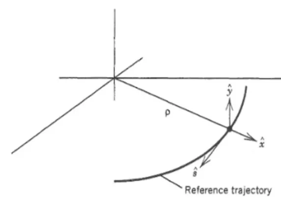
Figure 2.1: The new coordinate system for development of the transverse equations of motion.

profile. The resulting magnetic field is: ⃗

B = B′(y ˆx + xˆy), (2.1) where the field gradient B′ = ∂By/∂x = ∂Bx/∂y is evaluated at the center

of the quadrupole and ˆx, ˆy and ˆz (shown as ˆs in Fig. 2.1) are the unit vectors in the horizontal, vertical and longitudinal directions. For a charged particle passing through the center of a quadrupole, the magnetic field is zero. At a displacement (x,y) from the center, the Lorentz force on a particle with charge e and velocity v becomes:

⃗

F = evB′z × (y ˆˆ x + xˆy) = evB′y ˆy − evB′xˆx. (2.2) Thus, a focusing quadrupole in the horizontal direction (ˆx) is also a defo-cusing quadrupole in the vertical direction (ˆy) and vice versa.

2.1.2 Equation of motion

The description of transverse particle motion begins with a closed orbit, defined as the particle trajectory that closes on itself after one turn, and small amplitude oscillations around the closed orbit, called betatron oscil-lations. The closed orbit is defined by bending magnets (dipoles) which provide a path for a complete revolution of the particle beam. Since the bending angle of a dipole depends on the particle momentum (Bρ = pe), the resulting closed orbits will also depend on the particle momentum. Be-tatron motion around the closed orbit is determined by the arrangement of quadrupoles.

To properly write the equation of motion, a dedicated coordinate system is needed as is sketched in Fig. 2.1. Locally, the design trajectory (reference

(23)

2.1 Transverse beam dynamics 13 orbit) has a radius ρ and the path length along this curve is s. At any point along the reference orbit, three unit vectors can be defined: ˆs, ˆx, ˆy. The position of a particle is then expressed as a vector ⃗R in the form:

⃗

R = rˆx + y ˆy, where r ≡ ρ + x. (2.3) Let’s consider a generic particle with the correct momentum required for the experiment. This is called reference or synchronous particle. The coordinates defining its position and motion in the horizontal and vertical plane are respectively (x, x′) and (y, y′), where x′ = dx/ds and y′ = dy/ds represent the divergences from the reference orbit. In general, the equations of motion will be non-linear. But assuming only linear fields in x and y (such as dipoles and quadrupoles) and keeping only the lowest order terms in x and y, the linearized betatron equation of motion is given by the Hill’s equation: d2_x ds2 +  1 ρ2 + 1 Bρ ∂By(s) ∂x  x = 0 (2.4) d2y ds2 − 1 Bρ ∂By(s) ∂x y = 0. (2.5) Let (z, z′) represent either horizontal and vertical phase space coordinates. The equations above are both of form z′′ + Kz(s)z = 0, and differs form

a simple harmonic oscillator only in the “spring constant” Kz, which is a

function of position s. The general solution can be expressed in the form: z =Aβz(s) cos[ψz(s) + ψz(0)] (2.6)

where A and ψz(0) are constants to be determined from the initial conditions

and βz(s) is the betatron amplitude function. This is a pseudo-harmonic

os-cillation with varying amplitude βz(s)1/2 and the local betatron wavelength

is λ = 2πβz(s).

The phase advance is given by: ψz(0 → s) ≡ ∆ψ =  s 0 1 βz(s) ds, (2.7)

and thus, for a circulare machine, the number of oscillations per turn is Qz ≡ 1 2π  ₁ βz(s) ds, (2.8)

which is called betatron tune of the accelerator. If Qz were an integer

(24)

Figure 2.2: A resonance diagram for the Diamond light source. The lines shown are the resonances and the black dot shows a suitable place where the machine could be operated. Image courtesy J.A. Clarke et al, STFC Daresbury Laboratory.

the particle will be in exactly the same place each time it passes through the magnet, so this error will get amplified. These field errors cause the particle to take the wrong path and will eventually cause it to be lost. If the particle has an integer plus a half tune it will see this same error every second turn and integer plus a third will see the error every third turn and so on. Tunes in different planes can also combine to cause errors in the par-ticle path. The places where these tunes and combinations of tunes occur are called resonances. They are referred to as first, second, third order etc. referring to integer, half integer, third integer fractional tunes etc. The low-est order resonances are the most problematic. Most particle accelerators do not have to worry about tunes beyond about fourth or fifth order since the oscillations are usually damped on a sufficiently short time scale that they are not a problem. A simple example is shown in Fig. 2.2 where the lines represent the resonances and a good working place is indicated by a black dot.

It is useful to define other two new variables1: α ≡ −1 2 dβ(s) ds (2.9) γ ≡ 1 + α 2 β (2.10)

that together with β(s) compose the Courant-Snyder or Twiss parameters.

(25)

2.1 Transverse beam dynamics 15

Figure 2.3: The Courant-Snyder invariant ellipse defined by α, β, γ. The area enclosed by the ellipse is equal to ϵ. The maximum amplitude of the betatron motion is



ϵβ π and

the maximum angle isϵγ_π.

Using the new notation, it is possible to rewrite the Hill’s equation as: A = γz2+ 2αzz′+ βz′2 (2.11) where πA is the area of the Courant-Snyder invariant ellipse (see Fig. 2.3). The trajectory of particle motion with initial condition (z0, z0′) follows the

ellipse described by the Eq. (2.11). The phase space area πA enclosed by (z, z′) is constant at all places along the orbit while the shape of the ellipse evolves as the particle moves. After one turn, the ellipse returns to its orignal shape while the particle has propagated on the ellipse by a certain phase angle. The phase space area associated with the largest ellipse that the accelerator will accept is called the admittance. The phase space area occupied by the beam is called the emittance, ϵ = πA, and commonly measured in π · mm · mrad. The maximum displacement z and angle z′ at one point s along the orbit are given by:

z =  ϵβ(s) π and z ′ =  ϵγ(s) π . (2.12)

It is often convinient to speak of emittance for a particle distribution in terms of rms transverse beam size. Assuming a Gaussian particle distri-bution in both transverse degrees of freedom and an equilibrium situation where the distribution is indistinguishable from turn to turn, the emittance

(26)

is given by:

ϵ = −2πσ

2 z

β(s) ln(1 − F ) (2.13) at a point s where the amplitude function is β(s) and σz is the rms beam

size. F represents the beam fraction included in the phase space area ϵ. Measuring the transverse beam width σz (for example with an Ionization

Profile Monitor, IPM) the emittance can be calculated as: ϵ = σ

2 z

β(s) (2.14)

2.1.3 Momentum dispersion

We have just examined the motion of particles having the same mo-mentum as the ideal particle but differing in transverse position. What happens to a particle that differs in momentum by an amount ∆p = p − p0?

As already mentioned before, the bending angle of a dipole depends on the particle momentum. Thus, the resulting closed orbits are displaced from the reference orbit by an amount defined by the momentum dispersion function D(p, s). The displacement from the ideal trajectory of a particle due to the momentum spread is then given by:

x = D(p, s)∆p p0

+ xβ (2.15)

where the first term represents the new closed orbit of the off-momentum particle and the second the betatron oscillation about that closed orbit.

In addition, higher momentum particles are bent less effectively in the focusing elements. That is, there is an effect analogous to chromatic aberra-tion in convenaberra-tional optics. The dependence of focusing on momentum will cause betatron oscillation tune dependence on momentum. The parameter quantifying this relationship is called chromaticity and it is defined as:

δν = ξ(p)∆p p0

, (2.16)

where δν is the change in tune, ξ(p) is the chromaticity and ∆p/p the frac-tional momentum deviation from the synchronous particle. The source of chromaticity discussed here is the dependece of focusing strength on mo-mentum for ideal accelerator fields. This is called natural chromaticity. There are additional sources coming, for example, from field imperfections

(27)

2.1 Transverse beam dynamics 17 but they will not be treated here. It is important to worry about chro-maticity because if the beam has a large momentum spread, then a large chromaticity may place some portion of the beam on resonance where it will be lost.

In order to correct the chromaticity effect, what is needed is a mag-net that presents a gradient depending on the particle momentum. A dis-tribution of sextupole magnets is normally used for this purpose. In the horizontal plane, the sextupole field is of the form

B = kx2, (2.17)

and so the field gradient on a displaced equilibrium orbit is B′ = 2kx = 2kD∆p

p0

. (2.18)

Unfortunately, the sextupoles inevitably introduce non-linear aberrations which need a more complicated description than the linear dynamics briefly shown in this chapter.

Let’s emphasize here the role of betatron oscillations on the particle path length. This is a crucial contribution to the horizontal polarization lifetime, as will be explained in the next chapter.

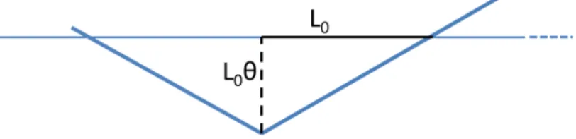
In general, a particle undergoing betatron oscillations travels a longer path compared to the ideal particle. Let’s consider the simplest example in one dimension. Fig. 2.4 shows the reference orbit (horizontal straight line) and the trajectory of a particle undergoing a betatron oscillation by drawing a triangle built on the design orbit. The length of the segment along the hypotenuse is L = L0

√

1 + θ2_{, where θ is the angle deviation}

from the central ray. If the angle is small, the Taylor series expansion of the square root produces ∆L/L0 = θ20/2, but this is an overestimate. The

velocity for the triangle path is a constant v > v0. In fact, the velocity

oscillates between these two extremes, remembering that this is added as a correction transverse to the main velocity around the ring. The best value then becomes the average of these two extremes, v and v0, since the

oscillation between them is sinusoidal. So there is another factor of 2 in the denominator. The X and Y contribution add in quadrature, so

∆L L0 = θ 2 x+ θ2y 4 . (2.19)

Since bunching the beam (see Sec. 2.2) keeps all particles on average isochronous, such oscillations lead to a longer beam path and a higher particle speed, thus changing the spin tune. This concept describes a fundamental contribution to the horizontal polarization lifetime.

(28)

Figure 2.4: Sketch of a betatron oscillation in one dimension. The horizontal straight line represents the design orbit and is the basis of a triangle describing the particle trajectory undergoing a betatron oscillation.

2.2 Longitudinal beam dynamics

In a storage ring after the acceleration process to the experimental en-ergy, the beam can be kept circulating in “packages” (bunched beam) or it can occupy the whole ring (coasting beam). In this section, the bunched beam case will be described since all the data presented in the thesis were taken under this condition.

The bunching process is obtained by using a radio-frequency (rf) cavity, which provides a longitudinal oscillating electric field. Phase stability en-sures the stability of the longitudinal motion for particles in the bunch that normally differ in momentum from the ideal one.

2.2.1 Phase stability

For a particle with charge e, the energy gain per passage through the cavity gap is

ϵ = eV0sin(ωrft + φs), (2.20)

where V0 is the effective peak accelerating voltage, ωrf is the rf frequency

synchronized with the arrival time of the beam particles and φs is the phase

angle. A particle synchronized with the rf phase φ = φs at revolution

period τ and momentum p0 is called a synchronous particle. A synchronous

particle will not gain/loose energy per passage through the rf cavity when φs = 0. Normally the magnetic field is ideally arranged in such a way that

the synchronous particle moves on a closed orbit that passes through the center of all magnets.

What happens to a particle with a slightly different momentum from the synchronous particle? Let L be the length of the ring circumference and v0 the synchronous particle velocity. The time τ needed for one complete

(29)

2.2 Longitudinal beam dynamics 19 deviation in L or v is: ∆τ τ = ∆L L − ∆v v0 . (2.21)

This means that a particle moving faster than the ideal particle will take less time to complete one turn. But if the path length is larger, this deviation will tend to increase the time to reach the rf cavity. The velocity deviation, can be expressed in terms of the fractional momentum deviation by

∆v v0 = 1 γ2  ∆p p0  . (2.22)

where γ is the relativistic factor. The orbit circumference can be larger for a particle of momentum slightly above the ideal particle momentum, since the magnetic rigidity (Bρ = pe) is proportional to the momentum. The fractional change in the orbit length for a given fractional change in the momentum is: ∆L L = αc ∆p p0 (2.23) where αc is the momentum compaction factor. Its value depends on the

accelerator design. The fractional change in τ can finally be expressed in terms of ∆p/p0 as: ∆τ τ =  αc− 1 γ2  ∆p p0 = 1 γ2 t − 1 γ2  ∆p p0 = η∆p p0 (2.24) where αc ≡ 1 γ2 t (2.25) η = 1 γ2 t − 1 γ. (2.26)

γt is the transition energy and it is a property of the accelerator design,

while η is the slip factor. Equivalently, Eq. (2.24) can be written in terms of the revolution frequency f0 (the number of turns per second):

∆f f0

= −η∆p p0

(2.27) Eq. (2.27) is the key to understanding the concept of phase stability, as it is shown in Fig. 2.5. Below the transition energy, when η < 0, a higher energy particle (∆p/p0 > 0) has a higher revolution frequency and it will arrive at

the rf gap before the syncrhonous particle. That makes φ < 0, the energy gain is ϵ < 0, and the particle slows down. Similarly, a lower energy particle (∆p/p0 < 0) will arrive at the rf cavity later and gain more energy relative

to the synchrounous particle. This process provides the phase stability of synchrotron motion.

(30)

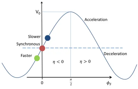
Figure 2.5: Schematic drawing of an rf wave, where the rf phase angles of a synchronous particle and the lower and higher energy particle are shown. For stationary motion, the phase stability requires φs= 0 for η < 0 and φs= π for η > 0.

2.2.2 Equation of motion

From the phase stability process, the synchrotron equations of motion can be derived. They are two difference equations describing the motion of a particle with arbitrary energy E and phase φ with respect to the syn-chronous particle: φn+1 = φn+ wrfτ η β2_E s ∆En+1 (2.28)

∆En+1 = ∆En+ eV (sin φn− sin φs) (2.29)

where the subscript n stands for the nth traversal of the rf cavity and ∆E = E − Es represents the energy difference between a generic particle

and the synchronous particle. (φ, ∆E) are pairs of conjugate phase-space coordinates. The demonstration can be found in D. A. Edwards’s and M. J. Syphers’s book in Ref. [17].

In Fig (2.6) the application of the synchrotron equation of motion is shown for 8 different initial enegies (∆E). In each case, the starting value of the phase is equal to the synchrotron phase. Several features are note-worthly. There is a well defined boundary between the confined and un-confined motion. This boundary is called the separatrix. The area in phase space within the separatrix is called a bucket while the collection of particles

(31)

2.2 Longitudinal beam dynamics 21

Figure 2.6: Application of the difference equations for synchrotron motion for a

sta-tionary condition (no acceleration). Each orbit represents a different initial condition. All of them start with the synchronous phase but different energies.

sharing a particular bucket is called a bunch. Finally, the harmonic number corresponds to the number of buckets.

The two difference equations, Eqs. (2.28) and (2.29), can be turned into one differential equation of the second order, assuming the turn number n as an independent variable. After a first integral and assuming ∆φ = φ − φs

being small, the equation becomes: d2_∆φ

dn2 + (2πνs)

2_{∆φ = 0} _(2.30)

where νs is the synchrotron tune, that is the number of synchrotron

oscilla-tions per turn. This quantity is given by:

νs=  −ωrfτ eV η cos φs 4π2_β2_E s , (2.31)

where η cos φs < 0 is the stability condition. The synchrotron oscillation

frequency is 2πf νs, where f is the revolution frequency, and it is much

(32)

(33)

Chapter 3 The COSY storage ring

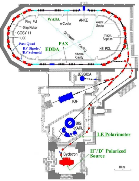
The COoler SYnchrotron COSY (see Fig. 3.1) at the Forschungszentrum-J¨ulich represents an ideal environment for the feasibility studies of the stor-age EDM experiment. For the experients described here, a deuteron beam was used.

It is a ring of 184 m length where two ion sources [18] provide polarized and unpolarized protons and deuterons. These beams are accelerated in the JULIC cyclotron and strip-injected into the COSY ring where they can be accelerated and used for the experiments in a momentum range from 300 MeV/c to 3.7 GeV/c. Electron cooling (electron energy 25-100 keV) at or near injection momentum and stochastic cooling covering the range from 1.5 GeV/c up to the maximum momentum are available to prepare monochromatic beams. The installation of vertical and horizontal dampers at COSY provides the possibility to stack electron-cooled beams and thus increase the beam intensity up to ∼ 1010 _{stored particles.}

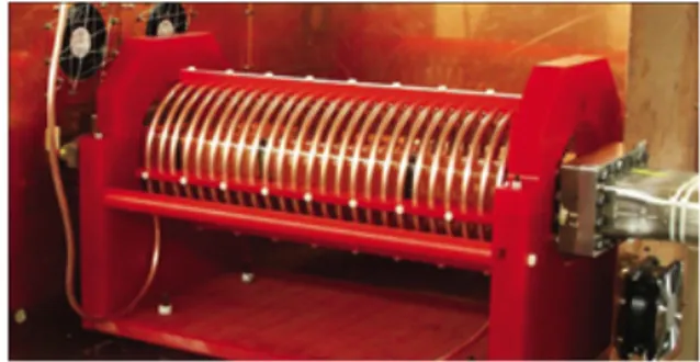
After the polarized source, the cyclotron accelerates the beam to the injection energy where the Low Energy Polarimeter (LEP) provides a pola-rization measurement of the states generated by the source. The rf solenoid (see Fig. 3.2) placed in one arc of COSY is a powerful tool to manipulate the beam polarization. Indeed, in the experiments presented in the next chapters, it was used to move the polarization from the vertical (stable) axis to the horizontal (ring) plane by inducing a spin resonance, whose fea-tures have been studied as a function of the emittance of the beam. Finally, the EDDA scintillator detectors (see Fig. 3.5) have been used as a mock EDM polarimeter to measure the vertical and the horizontal polarization components as a fuction of time, as is explained in the next section.

(34)

This chapter aims to describe the experimental setup and in particular the polarization measurements and the data acquisition systems used to record the data presented in this thesis.

Figure 3.1: The COSY ring. Starting from the bottom: the beam sources providing

polarized and unpolarized protons and deuterons, the cyclotron accelerating the beam to the injection energy, the low energy polarimeter (LEP) measuring the beam polarization, the COSY ring with the rf solenoid, and the EDDA polarimeter.

(35)

3.1 Experimental techniques and setup 25

Figure 3.2: The rf solenoid used to manipulate the beam polarization.

3.1 Experimental techniques and setup

3.1.1 Polarization measurement

For a beam of particles, the polarization is defined as the ensemble aver-age of the individual spins. In a spin-1 system [19] such as deuterons, there are three magnetic states along the quantization axis. In Cartesian nota-tion, the fractional populations of the deuterons in terms of the magnetic quantum number along some spin axis is given by f1, f0 and f−1, where

f1 + f0 + f−1 = 1. The unpolarized state is described by the condition

f1 = f0 = f−1 = 1/3, while the vector pV and tensor pT polarizations are

defined by

pV = f1 − f−1 and pT = 1 − 3f0. (3.1)

The range of the vector polarization pV is from 1 to −1, while the range

of the tensor polarization pT is from 1 to −2. Given that the sum of the

fractions has to remain 1, a pure vector polarization without tensor (f0 =

1/3) can only reach |pV| = 2/3. If a large tensor polarization is allowed,

values may reach |pV| = 1. These values may be reduced by any inefficiency

in the polarized source operation.

The polarization of a deuteron beam can be determined by measuring deuteron-induced reaction rates on a target, provided that the relevant an-alyzing powers (or sensitivities to the polarization) are sufficiently large. For the EDM experiment, the large vector analyazing power available with suitably chosen targets make it preferable to concentrate on this polariza-tion measurement rather than the tensor. Fig 3.3 shows the definipolariza-tion of the spin direction with respect to a coordinate system determined by the detected reaction products. The beam defines the positive ˆz axis. The loca-tion of the particle detector, along with the beam axis, defines the scattering plane and the direction of the positive ˆx axis. The scattering angle is β. In

(36)

Figure 3.3: The coordinate system for polarization direction (red arrow) based on the observation of a reaction product in a detector (small box). The beam travels along the ˆ

z axis. The detector position at angle β defines, along with the beam, the reaction plane and positive ˆx. The quantization axis for the polarization (red arrow) lies in a direction given by the polar angles θ and φ (as measured from ˆy axis).

this coordinate system we can specify the orientation of the deuteron beam quantization axis by using the two angles of a spherical coordinate system, θ and φ, where φ is measured from the ˆy axis and increases toward the positive ˆx axis. The interaction cross section between a polarized deuteron beam and an unpolarized carbon target is given by:

σ(β, θ, φ) = σunp(β)[1 + √ 3 pV iT11(β) sin θ cos φ + √1 8pT T20(β)(3 cos 2_{θ − 1)}

− √3 pT T21(β) sin θ cos θ sin φ (3.2)

− √

3

2 pT T22(β) sin

2_{θ cos 2φ]}

where the Tkq are the spherical tensor analyzing powers (k = 1 for vector,

k = 2 for tensor). Both the unpolarized cross section and the analyzing powers are properties of the reaction.

Measurement of vertical polarization The reaction is most sensitive to the vertical (along ˆy axis) component of the vector polarization when sin θ cos φ is near 1 or −1. If both pV and iT11are positive, for example, then

the rate at the detector (shown by the small box in Fig. 3.3) will increase relative to the unpolarized beam rate when sin θ cos φ ∼ 1. Likewise, a

(37)

3.1 Experimental techniques and setup 27 detector on the opposite side of the beam (on the −ˆx side) will see a reduced rate. The asymmetry in these two rates is a measure of the product pV iT11

and, for iT11 known, of the vertical component of pV. If the left and right

rates are L and R, then ϵLR =

√

3 pV,yiT11(β) =

L − R

L + R. (3.3) If positive (+ˆy) negative (−ˆy) vector polarization are available from the polarized source, the vector polarization can be determined from the cross ratio formula given by:

ϵCR = r − 1 r + 1 where r 2 = L(+)R(−) L(−)R(+), (3.4) and L and R are the count rates for the left and right systems for the positive (+) and negative (−) polarization states. Ths combinaion of count rates tends to suppress errors that arise as first-order contributions from geometric misalignments due to beam position or angle, or from detector acceptance.

Measurement of horizontal polarization If the polarization lies in the x-z plane or COSY ring plane, there will be a large and oscillating ˆx component of the deuteron polarization due to the precession of the mag-netic moment in the dipole fields in the ring. In a flat storage ring that is horizontal bending only, the stable spin direction is called spin closed orbit, ˆ

nco, and coincides with the vertical axis, orthogonal to the ring plane. Any

horizontal polarization component would precess about ˆnco while the beam

circulates in the storage ring. In a similar manner as described above, this will generate a difference in count rates for detectors mounted above and below the beam, such that

√

3 pV,xiT11(β) = ϵDU =

D − U

D + U. (3.5) Spin tune This asymmetry will oscillate with the g − 2 frequency. The number of spin precessions per turn about ˆnco is the spin tune, defined as:

νs = Gγ. (3.6)

The spin precession rate depends on the particle velocity through the rela-tivistic factor γ.

(38)

Figure 3.4: Starting from the left side, all the spins are alligned along the same direction so that the beam is horizontally polarized. After a while (right side), the spins spread out in the horizontal plane due to different particle velocities and thus different spin tunes. In this case, the horizontal polarization is lost.

Spin coherence time Let’s consider a particle beam, polarized in one direction in the horizontal plane (see Fig. 3.4). After some time, the spins go out of phase due to the momentum spread of the particles in the beam, making the horizontal polarization vanish. For the purpose of this the-sis, the horizontal polarization lifetime is the spin coherence time, the time during which the particle spins precess coherently around ˆnco while

main-taining some fraction of their initial polarization. In an EDM experiment where the longitudinal polarization must be aligned along the velocity, the horizontal polarization lifetime represents the time available to measure the EDM signal.

3.1.2 EDDA polarimeter

One concept for the EDM polarimeter involves stopping detectors that deliver their largest signals for elastic scattering events, since they are the most sensitive to spin interactions. In order to reduce the background of other processes such as break-up interactions, an absorbing medium between the target and the detector is installed. This arrangement was already developed in a previous experiment [20] using a thick carbon target (see Fig. 3.5) and the scintillators of the EDDA detector [21]. Long scintillators, called “bars”, run parallel to the beam and are read out with photomultiplier tubes mounted on the downstream end. These 32 scintillators are divided into groups of 8, corresponding to scattering to the left, right, down, or up directions. Outside the bars are “rings” that intercept particles scattering through a range of polar angles beginning at 9.1◦. Four consecutive EDDA rings were included in the “polarimeter group”, extending the sensitive angle range to 21.5◦. Over this angle range, the vector analyzing power for the elastic scattering of deuterons from carbon is positive and passes through the

(39)

3.1 Experimental techniques and setup 29

Figure 3.5: The carbon target used to extract the beam is placed in front of the EDDA detector. The left/right sectors are highlighted in light blue while up/down are in blue.

Figure 3.6: Deuteron elastic scattering cross section and vector analyzing power iT11

at 270 MeV [22].

first interference maximum [22] (see Fig. 3.6), making this an excellent range for operation as a polarimeter. The requirement that elastically scattered deuterons stop within the forward angle ring detectors led to the choice of 0.97 GeV/c as the optimum beam momentum.

Slow extraction In order to provide a continuous monitoring of the beam polarization during the storage time, the deuteron beam is slowly and con-tinuously extracted onto a thick carbon target (see Fig. 3.5), a carbon tube 15 mm long that surrounds the beam [20]. Slow extraction of the beam onto the target is achieved by locally steering the beam vertically upward into the top edge of the tube. Deuterons intercepting the target front face pass through the full target thickness, which greatly increases their probability of scattering into the EDDA scintillator system. This polarimeter scheme

(40)

offers a continuous monitor of the polarization during the beam store in contrast to previous experiments where observations were made at only one time during the polarization manipulation process [23].

3.2 Data Acquisition

3.2.1 Vertical polarization measurement

The triggers from the four segments (left, right, up, and down) of the EDDA detector were recorded in a single computer file for each run. A run consisted of a number of stores whose events could be added as a function of time since the start was synchronized to polarization precession operations through the use of a reproducible start time marker.

Analysis of the stores produced two cross ratio asymmetries, one for vector and one for vector-tensor polarized states. For comparison to the model calculations to be discussed later in Chap. 4, the two sets of cross ratio (see Eq. 3.4) data from each run were normalized to one based on the asymmetries recorded prior to any polarization manipulations being made. Then the two measurements were averaged. This combined all of the polarized beam data from a given run into one time-dependent set of vector polarization measurements.

3.2.2 Horizontal polarization measurement

The most critical new capability needed to measure the spin coherence time was the development of a “time-stamp system” which made possible recording the horizontal polarization as a function of time while it pre-cessed at 120 kHz. Thanks to the efforts of E. J. Stephenson, who prepared the project, and V. Hejny, who wrote the DAQ software, the first direct measurement ever of the rapidly rotating horizontal polarization was ac-complished.

A vertically polarized beam was injected into COSY and then the po-larization was rotated to the horizontal plane (null vertical popo-larization) using the rf solenoid operating at the spin resonance:

fres = fcyc(1 − Gγ) (3.7)

where fcyc is the cyclotron frequency and Gγ is the spin tune. The TDC,

(41)

Forschungs-3.2 Data Acquisition 31

Figure 3.7: Scatterplot of polarimeter events as a function of location around the

ring (vertical) and clock time in seconds (horizontal). There is sufficient time that parts of four different machine cycles are present. The intensity scale starts with violet and proceeds through blue, green, and yellow to red.

zentrum-J¨ulich) marked the polarimeter events with the elapsed time from a continuously running clock.

Particle position in the bunch The clock period of the TDC was 92.59 ps, a value much smaller than the COSY beam revolution time of 1.332 µs. This allowed good resolution on the longitudinal position of a detected particle within the beam bunch. Once the rf cavity signal and the TDC oscillator were cross-calibrated so that the turn number since DAQ start could be calculated, it became possible to use the fractional part of the turn number to provide a map of the particle distribution within the beam bunch. Fig. 3.7 is a scatterplot of polarimeter events as a function of location around the ring (vertical) and clock time in seconds (horizontal). It shows that as the cycles start, the beam is spread around the ring. The first few seconds are for injection, ramping, bunching, and the start of cooling. Bunching moves events out of the area near 300 and toward the center of the bunch near 1000 along the vertical axis. Electron cooling makes the bunch more compact (narrow yellow-red band). Outliers are slowly gathered into the main beam. After about 30 s, extraction of the bunch onto the polarimeter target starts. After that the height of the cooling peak declines until the beam is nearly gone. One machine cycle represents about 8.8 × 107 _turns.

(42)

Total spin precession angle For the next step, calculating the total precession angle, only the integer part of the turn number is used. A phase factor may be used to locate the break point in Fig. 3.7 so that the turn number does not increment in the middle of the bunch. The calculation of the total precession angle requires the knowledge of the spin tune frequency, Gγfcyc (about 120 kHz). This value may be obtained from the difference

between the rf solenoid resonance frequency and the cyclotron frequency (see Eq. 3.7). The rf solenoid spin resonance was determined at the beginning of the experiment using a variable-frequency Froissart-Stora [24] scan across the resonance (which flips the vertical polarization component) and refined with a series of fixed-frequency scans to locate the center of the resonance to within an error of about 0.2 Hz. With this as a start, the total horizontal polarization precession angle was calculated for each event as the product of the spin tune and the integral part of the turn number:

ωT OT = 2π Gγ Int(Nturns). (3.8)

Amplitude of D/U asymmetry The circle around which the polari-zation precessed was divided into 9 bins and polarimeter events from the up and down detector quadrants sorted separately into each bin. The ex-perimental challenge was the high frequency of the polarization precession. One full precession corresponded to only 6 turns of the COSY beam (about 8.3 µs) while the rate of the elastic scattered deuterons was approximately one in 700 turns. In order to provide some statistics, an accumulation time of 3 s was chosen and the down-up asymmetries were calculated for each bin and reproduced with a sine wave (see Fig. 3.8) of variable magnitude, phase, and offset (which is non-zero if there is a systematic difference in the detector acceptances):

D − U

D + U = f (ω) = A sin(ω + φ) + B. (3.9) The magnitudes from successive 3-second accumulation times were strung together to create a history of the horizontal polarization during the store. In the fitting of a sine curve to the down-up asymmetries, even a random distribution will produce a non-zero value of the amplitude. The so-called “positivity correction” of data will be described in Chap 5.

Spin tune refinement As a last refinement of the process, the spin tune itself was varied over a small range in each accumulation time to locate the value that gave the largest polarization magnitude. A peak was always

(43)

3.2 Data Acquisition 33

Figure 3.8: Sketch of the procedure to extract the horizontal polarization as a function of time from the total spin precession angle. On the left panel there are the sine waves, each of them used to fit a circle total spin precession angle accumulated for 3 s. On the right panel there is one example of the horizontal polarization measurement for three different beam emittances from a large (green) to a small (black) size. Each point of these curves corresponds to the amplitude of the sine wave, corrected for the “positivity” effect.

evident. Its FWHM was 1.8 × 10−6 of the value of the spin tune. Typically the spin tune would be known to 10−8 in each accumulation time and vary by 10−7 during a beam store. The variation appears to be associated with the changing spin tune across the profile of the beam as it is extracted onto the carbon polarimeter target.

(44)

(45)

Chapter 4 Study of an rf-solenoid spin

resonance

The search for an electric dipole moment using a polarized, charged-particle beam in a storage ring requires ring conditions that can maintain a longitudinal and stable polarization for long time. In fact, the EDM signal would be detected as a vertical polarization component arising from the rotation of the horizontal plane polarization toward the vertical direction. For the deuteron case, the detection of the EDM signal at level above one part per million requires a horizontal polarization lifetime, also called the spin coeherence time, of at least 1000 s.

The spin coherence time depends on the spin tune spread of the particles in the beam. As explained in Chap. 3, the spin tune, which is the number of spin precessions around the vertical axis during one turn around the ring, is proportional to the particle velocity as expressed by the relativistic factor γ. In a real beam, particles have different velocities and spins will precess with different frequencies. For this reason, the initial horizontal polarization of the beam will vanish with time because the spins spread out in the horizontal plane.

The feasibility of the deuteron EDM experiment depends on the mini-mization of the spin tune spread. In order to understand the mechanism which causes it, a series of polarization studies began at COSY. The first step was the analysis of a spin resonance curve and the measurements are presented in this chapter. Since the width of a spin resonance curve de-pends on the spin tune spread and thus on particle momentum distribution, each meachanism that can change the particle velocity in the beam could contribute to the spin tune spread. In particular, these mechanisms are

(46)

betatron oscillations which are due to the beam emittance and synchrotron oscillations that are present only in a bunched beam.

This study can be performed using either a coasting beam or a bunched beam.

In the first case, the particle beam is injected in the storage ring and it occupies the entire circumference. The main effect to the spin tune spread comes from ∆p/p (the fractional change in momentum respect to the reference particle) which kills the spin coherence time in milliseconds (∼ (fcyc∆p/p)−1). In this case there is no direct effect from the beam

emit-tance on the momentum spread, since particles off from the reference orbit will undergo betatron oscillations simply covering a longer path compare to the reference particle.

For a bunched beam, the framework is completely different. An rf cavity confines the particles inside a bucket, as described in Chap. 2. Particles with a different velocity from the reference particle will undergo synchrotron oscillation inside the bunch such that the first order effect of ∆p/p averages to zero. The path lengthening due to betatron oscillations forces the par-ticles to go faster in order to respect the isochronous condition introduced by the rf cavity. Thus, this effect can be described as a second order contri-bution from the beam emittance in the vertical and horizontal direction. A second order contribution from ∆p/p exists but is expected to be negligible compared to transverse size of the beam. The bunched case appears then to be a good solution in order to separately study the different contributions to the spin tune spread.

The tests at COSY made use of a bunched polarized deuteron beam with a momentum p=0.97 GeV/c. In order to provide a continuous measurement of the polarization as a function of time, the beam slowly extracted into a thick carbon target, placed in front of the EDDA detector. The vertical polarization was perturbed by a longitudinal radio-frequency (rf) magnetic field, inducing an rf depolarizing resonance which can flip the spin direction of stored polarized particles. The resonance frequency is defined as:

fres= fcyc(k ± Gγ) (4.1)

where fcyc is the cyclotron frequency and k is an integer. The studies

began by exciting the 1 − Gγ resonance and different tests were run at fixed and variable rf-solenoid frequency. Using a bunched beam, we compared the results obtained in case of electron-cooled and uncooled beam, since cooling shrinks the transverse sized of the beam and reduces the momentum spread ∆p/p. The data analysis was based on a simple no-lattice model

Spin Coherence Time studies for the storage ring EDM search

Universit`

a degli Studi di Ferrara

Spin Coherence Time studies

for the storage ring

EDM search

Contents

Introduction

Chapter 1

The Electric Dipole Moment as

a probe of CP violation

1.1

Baryon asymmetry

1.2

CP violation in the SM and beyond

1.3

The EDM as probe of new physics

1.3.1

Theoretical predictions

1.3.2

Experiments

1.4

EDM search in storage rings

Chapter 2

Elements of accelerator physics

2.1

Transverse beam dynamics

2.1.1

Strong focusing

2.1.2

Equation of motion

2.1.3

Momentum dispersion

2.2

Longitudinal beam dynamics

2.2.1

Phase stability

2.2.2

Equation of motion

Chapter 3

The COSY storage ring

3.1

Experimental techniques and setup

3.1.1

Polarization measurement

3.1.2

EDDA polarimeter

3.2

Data Acquisition

3.2.1

Vertical polarization measurement

3.2.2

Horizontal polarization measurement

Chapter 4

Study of an rf-solenoid spin

resonance