DIPARTIMENTO DI SCIENZE PURE E APPLICATE
CORSO DI DOTTORATO DI RICERCA IN SCIENZE DI BASE E APPLICAZIONI
Currriculum SCIENZA DELLA COMPLESSITÀ
CICLO XXXII
Analysis and forecasting of the structure of marine
phytoplankton assemblages using innovative molecular
techniques of NGS (Next Generation Sequencing) and
Machine Learning
Settore Scientifico Disciplinare: BIO/07
RELATORE
Chiar.ma Prof.ssa Antonella Penna
CORRELATORE DOTTORANDO Chiar.mo Prof. Michele Scardi Dott.ssa Eleonora Valbi
Index
Abstract ... 1
Preface ... 3
1.
Itroduction ... 5
1.1.
Marine Phytoplankton... 5
1.2.
Ocean Sampling Day ... 8
1.3.
Harmful Algal Blooms ... 9
1.4.
General characteristics of dinoflagellates ... 12
1.5. Alexandrium minutum ...
.... 13
2.
Methods ... 15
2.1.
Mathematical models and Machine Learning ... 15
2.2.
Main methods used in the present thesis ... 16
2.2.1. Random Forest ... 16
2.2.2. Cohen's K coefficient and CCI ... 19
2.2.3. Roc curve and AUC ... 20
2.2.4. Similarity, distance and association coefficients ... 21
2.2.5. Hierarchical clustering ... 24
2.2.6. Space-constrained clustering and Gabriel graph ... 25
2.2.7. Ordination methods and Principal Coordinates Analysis 26
2.2.8. PERMANOVA ... 28
2.2.9. Mantel Test ... 29
2.2.10. Procrustes test (PROTEST) ... 30
3.
Results ... 32
3.1.
Predictive model for A. minutum occurrence ... 32
3.2.
OSD data analysis ... 33
4.
Discussion and conclusions ... 47
5.
Acknowledgements ... 49
6.
References ... 50
1
Abstract
The work carried out during these three years of Ph.D. followed two different objectives: the development of a predictive model for the occurrence of the toxic algal species Alexandrium minutum and the study, through data analysis techniques, of phytoplankton biodiversity at a global and local level, with particular interest into the European area.
Regarding the first of the two objectives, a predictive model was developed using the Random Forest technique. For this purpose, data relating to A. minutum occurrence, detected by the PCR technique carried out on samples of water taken in the NE Adriatic Sea area, and data relating to the different predictive variables, were provided to the program. Precisely, two models have been developed, one using 18 predictive variables, including the values of different nutrients, and one using only 12 of the 18 variables, excluding nutrient values, in order to a more easily use of the model in future, without the need for laboratory analysis. Results show that both models have good reliability values and that the 12-variable model works as well as the 18-variable one and can therefore be used without the risk of losing essential information. A work exposing these results has been published in the journal "Scientific Reports".
Regarding the second of the two objectives, we examined data relating to the OSD campaign, an international project that provided for collecting, by different partners all over the world, sea water samples during the day of summer solstice. Samples were analyzed with metagenomic techniques, which led to the identification at the genus level of the different organisms present within the samples. After a firts exploratory analysis, in which data were analyzed using the Principal Coordinates Analysis technique, starting from a matrix obtained with to Jaccard coefficient between the different stations, the dataset was divided into clusters, thanks to a space-constrained clustering bound by a matrix of geographical connections obtained from a Gabriel graph. Subsequently, we decided to focus our attention on the two Longhurst ecoregions that had the
2
greatest number of samples, namely Mediterranean Sea and NE Atlantic Shelves Province, looking for associations between taxa. Two different association matrices, one for each province, were created using the Fager & McGowan coefficient and were subsequently analyzed using the Mantel test. The test result found a certain correlation between the two matrices. On the same line, also the result of the PROTEST performed on the two ordination originating from the two matrices. This suggests that associations between different taxa, more than being linked to the geographical position in which they are located, depend on other issues, such as, for example, the physical characteristics typical for every taxon. A manuscript presenting this work and its results is currently being drafted.
3
Preface
The research project provided, from its initial draft, two objectives: (i) the formulation of a predictive model for the occurrence of the toxic microalgal species, Alexandrium minutum Halim, 1960, in the NE Adriatic Sea, and (ii) an exploratory study of metagenomic data, related to the phytoplankton biodiversity at a global level, with particular attention to community structures and associations among the different taxa.
The work carried out during the first year of the Ph.D. program focused mainly on the first of the two objectives and concerned the training and the validation phases of the model.
The first months of the second year of the Ph.D. were focused on improving the performance of the previously developed predictive model. Subsequently, a manuscript was drawn up for the dissemination of the obtained results, addressing it to the journal "Scientific Reports". The work was therefore accepted and published, on March 12, 2019, as "Valbi E., Ricci F., Capellacci S., Casabianca S., Scardi M., Penna A. (2019). A model predicting a PSP toxic dinoflagellate occurrence in the coastal waters of the NW Adriatic Sea.".
During the period concerning the last semester of the second year and the whole third year of the Ph.D., the work focused on the second objective of the project, using the sequences of the genes encoding the 18S rRNA of the phytoplanktonic organisms found in sea water samples taken in the Ocean Sampling Day (OSD) campaigns in various areas of the world. A manuscript summarizing the results obtained is currently in the drafting phase.
Therefore, the Results paragraph of this Ph.D. thesis, will be divided into two parts: the first one concerning the developed predictive model, in which the
4
published article will be attached, the second one which will include all the results of the various exploratory analysis carried out on OSD data.
5
1. Introduction
1.1. Marine Phytoplankton
Oceans and seas cover 70% of the global earth's surface and constitute the largest continuous ecosystem on earth, accounting for 95% of the volume of the biosphere. The microbial communities that populate them make up about 90% of the marine biomass and play a fundamental role for life, not only in the aquatic environment, but also on land.
Firstly, the micro-organisms are involved in the biogeochemical cycles, oxidation and reduction processes of the chemical elements that allow the recycling of matter within the ecosphere. In particular, the fotoautotrophic part of the microorganisms present in the marine ecosystem, namely the phytoplankton, represented by microalgae and cyanobacteria, living near the surface where there is enough light to allow photosynthesis, is responsible for about the 50% of the
global primary production (Falkowski et al. 1998; Behrenfeld et al. 2001;
Falkowski & Raven 2007). Through photosynthesis, phytoplankton uses solar radiation and inorganic nutrients to convert inorganic carbon into organic carbon, releasing oxygen and producing biomass. For this reason, phytoplankton serve as the basis of the marine pelagic food web and, therefore, it is in a central role to life in the oceans (Field et al., 1998, Seymour, 2014). With such a leading role, it seems clear that any alteration to phytoplankton can potentially impact on the
whole ecosystem. Moreover, biomass production, being the basis of fish
production, strongly influences the fishing sector and therefore a considerable part of the local and global economy.
In addition to indirectly benefit from the phytoplankton ecosystem functions, man uses marine ecosystems even directly, in the blue biotechnologies, for the development of new products with high economic value.
6
For example, microalgae have the potential to provide a new range of third generation biofuels; they can be used for the treatment of wastewater and industrial waters and in bioremediation programs of contaminated environments. While in the healthcare field marine microorganisms are used for the production of enzymes, drugs (antiviral and anticancer), cosmetics and nutraceutical compounds.
Water masses are contiguous on the planet, but the composition and the abundance of phytoplankton is significantly different in space and time (Gran, 1912).
The variability of phytoplankton depends on many mechanisms, such as the physiology of the organism and its life cycles. Carbon dioxide, sunlight, and nutrients availability are the factors that mainly influence phytoplankton growth, and its distribution may also be affected by the physical environment and the interaction with other organisms (Margalef, 1974). Human activities and global climate changes are now potent new drivers that significantly affect the functioning of coastal and offshore marine ecosystems, too (Hallegraeff, 2010; Huertas et al., 2011; Sunday et al., 2014).
Being the phytoplankton at the base of marine trophic webs, the analysis of its populations has a very important role. Eventual alterations to the community, in fact, can modify the structure and the functioning of an entire ecosystem.
Studying and knowing phytoplankton biodiversity and its community structure, with the dual purpose of being able to benefit from it and preserve it, is today of crucial importance.
Unfortunately, despite their high value, to date there is still little information on most marine microorganisms, their functions and ecological interactions between the different species, since most of these are not, or are difficult to cultivate under laboratory conditions, thus making it impossible to study its physiology.
7
In studies of microbial communities, this difficulty in cultivating certain phytoplankton strains inevitably turns into a loss of information. Not being able to cultivate it, we lose the information on the occurrence of a specific micro-organism is, obtaining a list of very reduced species, compared to the number naturally present in the reference sample. A further problem could also arise in the case of cultivable strains, since traditional microbiology techniques often involve a first phase of enrichment of the environmental sample and the subsequent isolation of the single species present.
It is therefore evident that already in the choice of the culture medium and the pre-enrichment conditions a selection is made in favor of some microbial species, with physiological needs similar to the selected conditions, but which do not necessarily represent the organisms or the organism that prevails in the environment. Another problem could be given by the probability that many of the microorganisms present in the environmental sample are not able to grow in pure cultures as they need to live in microbial consortia. Furthermore, it must be considered that the maintenance costs of microalgal strains in culture are usually very expensive.
Problems of this kind can be overcome, and in fact have already been overcome in recent decades, thanks to the advent of metagenomics, through which innovative techniques of culture-independent molecular biology have been developed, allowing us to collect a great deal of information on marine biodiversity.
Metagenomics is the study of the genomes of microbial communities directly in their natural environment, through the amplification of the present DNA and the subsequent sequencing of specific target regions. This avoids the need for isolation and cultivation of individual species.
Unlike the first techniques developed in the 1980s and 1990s, which involved the cloning of specific sequences (Sanger et al, 1975), the current techniques of Next Generation Sequencing (NGS) analyze in parallel thousands or millions of DNA sequences or RNA, without having to clone them in bacterial systems. In particular, the Illumina MiSeq® methodic, based on Sequencing By Synthesis (SBS), allows us to analyze millions of sequences in a few hours with maximum
8
accuracy and yield without reading errors. In this way it is possible to know all the biodiversity present in a given sample, being able to identify, in addition, many species of microorganisms that were once unknown.
These large amounts of information now available (called big data), included in international databases and easily accessible to scientists from around the world, can be used for exploratory studies on biodiversity and community structure.
1.2. Ocean Sampling Day
The idea for the second objective of the Ph.D. project came from the availability of data obtained from the OSD campaign.
The OSD is part of a European project, the EU 7FP Micro B3 (Marine Microbial Biodiversity, Bioinformatics, Biotechnology) based on an interdisciplinary consortium of 32 academic and industrial partners including world experts in bioinformatics, informatics, biology, ecology, oceanography, bioprospecting and biotechnology and legal aspects.
The multiple purposes of this international project are: the study of marine biodiversity, the development of innovative bioinformatics approaches to make data of the genomes of viruses, bacteria, archaea and marine protists and of the metagenomes of marine ecosystems available and the definition of new targets for biotechnological applications.
All samples were collected on a simultaneous sampling campaign of the world’s oceans which took place on the summer solstice (June 21st) in 2014 and was repeated in 2015.
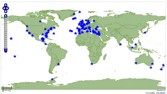
191 sampling sites participated in OSD on June 21st, 2014 (Kopf et al., 2015) and
most of them joined again in 2015. These sites range from tropical waters to polar environments (Fig. 1).
9
The University of Urbino also actively took part in the project, contributing with a sampling carried out by the Environmental Biology laboratory of the Department of Biomolecular Sciences, along the coast of Pesaro.
All the collected samples were sent for metagenomic analysis and data, available on a global scale, were loaded into a database on the ENA-EMBL database. The dataset includes the list of the different sequences of genes present in each station, the assignment of a taxonomic group of the sequences has been possible up to the genus level for most of the records, while for the remaining ones it has arrived at higher taxonomic levels .
The dataset contains both zoo- and phytoplankton, eukaryotic and prokaryotic species. For this work only the phytoplankton eukaryotic ones were considered, leaving the others aside.
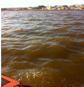
1.3. Harmful Algal Blooms
In recent decades, worldwide, coastal systems have been facing a variety of environmental problems, due to the highly increasing of anthropic pressure. Some
10
of these problems are
degradation or destruction of coral reefs and seagrass meadows (Boudouresque et
al., 2012, Bacci et al., 2014),
decreasing quality of coastal waters for recreational use, depletion of fish stocks
(Pauly et al., 1998) and
Harmful Algae Blooms
(HABs) events (Smayda and
Reynolds, 2001, Bricker et
al., 2003,Kudela and Gobler, 2012, Wells et al., 2015) (Fig. 2).
HABs are caused by microalgae fast proliferation that has a negative impact on human activities.
When microalgae find suitable physical, biological and chemical conditions for
growth, they can quickly reach high concentrations (104–105 cell L-1) in a short
period of time (commonly 1–3 weeks).
There are two types of harmful effects and harmful species can be related to one or both characteristics: high-biomass production and toxin production.
High biomass blooms affect the biota, causing fish kills and, therefore, influencing fishing and aquaculture industry (Hoagland and Scatasta, 2006,
Berdalet et al., 2015) and causing economical problems connected to the
deterioration of the coastal recreational waters.
Marine biotoxins are represented by a heterogeneous group of chemical compounds, structurally different from each other, but with common characteristics. Generally they are stable to heat and acidic environment. A generic division of these compounds can be based on their solubility,
11
distinguishing them in water-soluble biotoxins and liposoluble ones (Poletti et al.,
2003).
Toxic syndromes in humans are caused by either the inhalation of aerosols (Gallitelli et al., 2005, Ciminiello et al., 2015) or the consumption of mussels, claims and oysters contaminated, that, being filter feeders, accumulate high concentration of these toxins in their digestive system.
Harmful species belong to six algal groups (diatoms, dinoflagellates, haptophytes, raphidophytes, cyanophytes, and pelagophytes) each with a specific morphology,
physiology and ecology (Zingone and Enevoldsen, 2000; Garcés et al., 2002).
Toxins produced by marine dinoflagellates are the most powerful non-protein
poisons known (Steidinger, 1983; Steidinger and Baden, 1984; Anderson and
Lobel., 1987).Several studies highlighted the importance of the biotransformation
processes of algal toxins by molluscs and fish. In fact it has been shown that the metabolism of these animals can change the chemical structure of the toxin, causing a change in the toxic effect, making it forty times more powerful (Ade et
al., 2003). Currently, approximately 2000 cases of intoxication (with a 15%
mortality rate) in humans due to consumption of toxic shellfish or fish are registered annually (Hallegraeff et al., 1995).
Human pressure may influence the increasing of HABs events in different ways: transporting resting cysts of toxic species from a place to another, even very far, with ballast water and floating plastic, causing eutrophication, an over-enrichment
of nutrient of the water (Smayda, 1989, Hallegraeff, 1993), inducing climate
changes, exploiting the coastlines (Vila et al., 2001, Garcés et al., 2002),
overfishing.
The HAB monitoring programs recently increased (Anderson et al., 2012a) but, although many affected areas are well monitored, other are less controlled. Moreover, monitoring operations are often very expensive.
A great help about it may come from mathematical models, that are now able, with a high percentage of confidence, to predict these events. The use and
12
improvement of these techniques will be the next challenge in the upcoming future (Kleindinst et al., 2014).
1.4. General characteristics of dinoflagellates
Dinoflagellates are a group of microscopic algae mostly unicellular and flagellated, which represent one of the most important phytoplankton groups both marine and freshwater with over 2000 living species. The cells are characterized by the presence of an outer membrane below which there is a layer of flattened
vesicles (amphiesma), which may contain cellulose plaques. The
presence/absence, the number, the layout and the morphology of the plates are a
very important character for the classification(Steidinger and Tangen, 1997; Boni
et al., 2005).
The cell is divided into two distinct parts (Fig. 3): the epitheca is the upper part, which in some species can be very small and the ipotheca is the lower part (epicone and hypocone, respectively, in athecate species). These two parts are divided by a transverse septum called a cingulum. In the ventral part of the cell there is a longitudinal septum, called sulcus which starts from the cingulum. Some species have expansions, similar to sails, which originate from the two septa, probably to favor floating. Two flagella, which originate from a flagellar pore
located where the cingulum and the sulcus converge, give the name to the group.
The life cycle of dinoflagellates has both asexual and sexual reproduction. In unfavorable conditions, the zygote can form a durable and resistant structure to the external environment: the cyst, which can remain in a dormant stage for a long time, and then begin vegetative reproduction once the environmental conditions
13
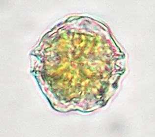
1.5. Alexandrium minutum
The species studied in this
doctoral thesis is the
dinoflagellate Alexandrium
minutum Halim, 1960 (Fig. 4),
the most widespread toxic
species in the western
Mediterranean basin (Giacobbe
and Maimone, 1994, Vila et al.,
2001). It can produce saxitoxins, GTX1 and 4, that can cause a
severe human illness, the
Paralytic Shellfish Poisoning
(PSP) syndrome (Wiese et al., 2010, Perini et al., 2014), the most widespread HAB-related shellfish poisoning illness (Anderson et al., 2012b), as well as one of the most studied and known syndromes because of the serious consequences that produces in consumers of bivalve molluscs. The onset of symptoms occurs in the thirty minutes following ingestion with paresthesia to the mouth, lips, tongue,
Fig. 3: Typical (a) athecate and (b) thecate dinoflagellate cells in ventral view. From: Salmaso and Tolotti, 2009.
Fig. 4: The dinoflagellate Alexandrium minutum PSP producing species.
14
extremity of the limbs, profound muscular asthenia, inability to maintain an upright position. In fatal cases death occurs after 3-12 hours for respiratory paralysis. Patients that survive the first 12 hours, regardless of the amount of toxin
ingested, usually recover quickly without other effects (Toyofuku, 2006). The
severity of the symptoms depends on the amount of toxin that has been ingested. Symptoms are classified into moderate, severely moderate, and severely extreme. For the moderate the amount of saxitoxin varies from 2 to 30 μg / kg, while in the
other cases the quantity varies from 10 to 300 mg / kg. (Tubaro and Hungerford,
2007).
The presence of A. minutum has been reported from coastal waters in various locations in the northern hemisphere, including Turkey, ltaly, Spain, Portugal, Ireland, The Netherlands, Germany, and the Atlantic coast of North America (Nehring, 1994), as well as from Australasian waters (Bolch et al., 1991; Chang et
al., 1995).
This species has been responsible for toxic blooms along the northwestern coast of the Adriatic Sea (Italy) and Ionian Sea, where mussel farms have been contaminated (Honsell et al., 1996, Penna et al., 2015).
15
2. Methods
2.1. Mathematical models and Machine Learning
Natural phenomena can be expressed in mathematical language thanks to the use of models.
Their applications are used both for the synthesis and the description of knowledge and for predictive purposes.
The development of a mathematical model involves three fundamental phases
(Guisan & Zimmermann, 2000):
formulation. The starting point is, of course, an ecological concept. In order to
carry out an adequate formulation of the model it is fundamental to choose the variables to be analyzed, as well as an adequate space-time scale;
calibration. The ultimate goal of creating a mathematical model is to obtain the best possible accuracy. To achieve this, during this phase the values of the different parameters involved in the creation of the model are optimized;
validation. Once the model has been formulated, its accuracy must be verified.
In this phase various statistics are used for the purpose.
Given the considerable amount of information available today, it is becoming necessary to use mathematical models that exploit the increasingly efficient calculation tools. In particular, models that fall within the field of Machine Learning have proved to be very useful.
The term Machine Learning focuses the attention on the ability of computers to learn automatically from experience, mimicking what happens in human learning processes. In computer programs, performance is improved using experience, namely the available data that is provided to the algorithm (Alpaydin, 2014). What you get is a generalizable result, which can be used by entering new data, unknown to the machine.
16
supervised, which includes trained algorithms starting from the analysis of one
or more response variables. The training is based on the informations provided in input, which are both those relating to the predictive variables, and those
relating to the response, which is therefore known. The learning process
generates hypotheses that can be used in the future to predict unknown cases, in which only the data relating to the predictive variables are available and the
response variable is to be known. (Omary & Mtenzi, 2010). Examples of this
type of learning can be Decision Trees, K-Nearest Neighbour (KNN), Support Vector Machines (SVM), Artificial Neural Networks (ANN) e Random Forests;
unsupervised. This type of learning includes algorithms that analyze data
without any predefined response example (Omary & Mtenzi, 2010), as in the
case of some types of Neural Networks (Self Organizing Maps) and of different non-hierarchical classification algorithms.
2.2. Main methods used in the present thesis
2.2.1. Random Forest
Regarding the predictive aspect, the technique considered most suitable for the
development of the model is the Random Forest (RF) (Breiman, 2001). This
technique is based on a set of Classification Trees (CT), which are combined together to obtain predictions, formulated as the observations probability of belonging to the various response classes (Cutler et al., 2007).
In case of predictive models for the occurrence of a given species, such as that examined in this thesis, the response classes are only two, presence and absence.
Each tree is characterized by the presence of splits which represent as many conditions.
17
In the specific case of a binary classification, there are only two responding alternatives to a given condition. Therefore, at each split a randomly chosen variable is taken into account and data are divided into two groups based on the value of the variable associated with them. Data will be assigned to one or the other class depending on whether the value of the said variable is higher or lower than a given threshold value, suitably defined by the algorithm so as to obtain the best possible division. The first split is followed by others, in which the data is subdivided again based on the value of one of the predictive variables, or even the same, but whose discrimination threshold is different. Finally, the tree ends with leaves, which contain the probability of belonging to each response class.
Variability is not only given by the high number of CTs combined by the RF. In fact, each tree randomly selects only a subset of data from the input set and a subset of predictor variables to be analyzed is selected for each node (Peters et al., 2007).
Every single CT provides an answer, expressed as the probability of belonging to different classes. The various responses are combined together by the RF, whose output will therefore depend on the complex of those of the CTs that form it. The result of each of the different CTs is considered as a "vote". In practice, a RF creates its output based on the majority of the predictions of the trees that constitute it.
The training of the model is represented by a process in which the conditions characterizing the splits, the total number of CTs and the minimum number of cases present within each leaf (size) are defined and optimized.
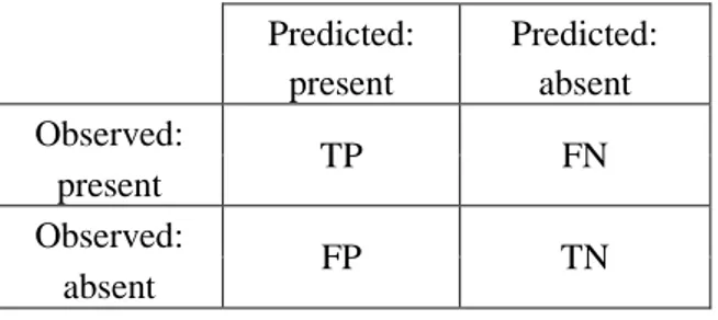
At the end of the training, the program creates a particular contingency table, the confusion matrix (Tab. 1), in which each cell represents the combinations of observed or predicted data.
As already mentioned above, in this doctoral project a model was developed in which the RF response classes are only two. For this reason, the examples given
18
in this thesis concern this particular type of model, whose confusion matrix has a 2×2 dimension. Predicted: Predicted: present absent Observed: TP FN present Observed: FP TN absent
Thus, four distinct cases are obtained:
TP: true positives The observed and the predicted data correspond and are both positive, i.e. they are both presence cases;
TN: true negatives. Even in this case, observed and predicted data correspond,
but both are cases of absence of the studied species;
FP: false positives. There is no concordance between observed and predicted
data. The model predicts presence, but in the observed data the species is absent;
FN: false negatives. Also in this case there is discrepancy. Predicted absent, observed present.
Model validation is based on two different approaches (Guisan & Zimmermann,
2000): il primo prevede l’uso di un singolo set di dati, con cui viene effettuata sia la calibrazione sia la validazione; il secondo prevede l’impiego di due distinti set di dati, il training set, usato durante la calibrazione, e il test set per la validazione (Manel et al., 1999).
The first approach is generally chosen when the initial data set is not large enough and the model is validated by randomly extracting small subsets of data that vary during the training (cross-validation). If, instead, the initial data set is large enough, so that it can be divided into training sets and test sets, then it is possible to carry out a real validation.
19
Once the model is trained, its predictive ability must be tested. For this purpose
are useful Correctly Classified Instances (CCI), Cohen's K coefficient (Cohen,
1960)and the Receiver Operating Characteristic (ROC) curve(Zweig e Campbell,
1993) are useful. In this study there was a subdivision of the original dataset in training and test set and the necessary tests were carried out on the test set results.
2.2.2. Cohen's K coefficient and CCI
Cohen's K coefficient is a statistic used to evaluate the accuracy of the model, measured as the level of agreement between observed and predicted data. It is defined by the author as the proportion of expected disagreements based on the hypothesis of a random association between observed values and expected values. particularly, K is defined as:
p1 is the overall proportion of expected concordance cases;
p0 is the overall proportion of cases of agreement expected under the
hypothesis of random association.
K value, therefore, ranges from 0 to 1 and each interval of values corresponds to a level of agreement:
0 ≤ K < 0.2 the agreement is poor;
0.2 ≤ K < 0.4 the agreement is fair;
0.4 ≤ K < 0.6 the agreement is moderate;
0.6 ≤ K < 0.8 the agreement is good;
0.8 ≤ K ≤ 1 the agreement is very good.
Correctly Classified Instances (CCI) is defined as the proportion of correctly predicted cases, often also referred to as sensitivity.
20
2.2.3. Roc curve and AUC
Species is default considered present by RF if at least 50% of the CTs "voted" classifying it as present. However, in cases where, as in ours, the absence data in the original dataset are more than those of presence, the RF learns better to classify the former than the latter.
This results in an imbalance of the results towards false negatives, i.e. cases in which the species is predicted as absent, but it is present, with a consequent decrease in the accuracy of the model. To overcome this problem, we used ROC curve to define the optimal threshold value of discrimination between presences and absences.
This technique relates two important indices, sensitivity and specificity, both calculable starting from the confusion matrix:
sensitivity is the proportion of presence cases that have been correctly
predicted (Smith, 2012), namely true positives;
specificity is the proportion of absence cases correctly predicted (Manel et al.,
1999), namely false negatives.
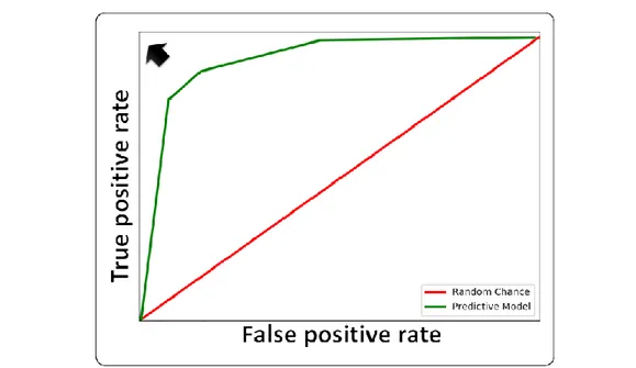
In an XY graph, all the possible threshold values analyzed are plotted, taking the corresponding specificity values as coordinates on the x-axis and the sensitivity values on y-axis. By joining the points you will get a curve, namely the ROC curve. The optimal threshold value will be given by the cut-off value associated with the ROC curve point which has the maximum distance from the diagonal, which corresponds to the point where the true positives are minimized and the false negatives minimized (Fig. 5).
The area below the ROC curve is defined as Area Under the Curve (AUC), which can be a very useful measure to evaluate the performance of a model based on presence/absence data (Manel et al., 2001). The AUC has a range that varies from a minimum of 0.5 up to a maximum of 1. According to the Swets classification (1988):
21
AUC = 0.5: the model is non-informative;
O.51 < AUC < 0.7: the model has low accuracy; 0.71 < AUC < 0.9: the model is accurate;
0.91 < AUC < 0.99: the model is highly accurate;
AUC = 1: the model is perfect.
2.2.4. Similarity, distance and association coefficients
When data matrix is composed of several variables such as, for example, a list of species, in order to evaluate the differences among observations, the original matrix is turned into a similarity or distance matrix, using a similarity or distance index, which calculates the differences between all the different pairs of observations. The choice of the right measure of similarity or distance is of fundamental importance.
Similarity coefficients express the similarity between two samples, assuming values that vary between 0, in the case of completely different observations, and
Fig. 5: Representation of a ROC curve. Ideal model (marked by an arrow); hypothetical curve (green) and random chance, diagonal line (red). From: Prieto-Martínez et al., 2018.
22
1, in the case of observations that fully satisfy the criterion used, not necessarily identical to each other.
Distance coefficients measure the differences between two observations and can take values ranging from 0, in the case of identical observations, to a variable value depending on the coefficient, for different observations.
Similarity measures can be transformed into dissimilarity measures, taking their complement to 1. Only some of these, however, own the metric properties typical of true distance coefficients, which allow to order the observations in a Euclidean space, through ordination methods.
Among the available coefficients symmetrical and asymmetrical ones can be distinguished.
This is a very important distinction and the use of one or the other type depends on the nature of the available data.
In ecological studies it can easily happen that for one or more descriptors there are null values. In some cases these correspond to a certain datum, at least within the limits of the error of sampling and determination methods (e.g. the absence of a pollutant). In other cases, instead, especially when analyzing lists of species, zero suggests more the absence of information. This can be due to the previously exposed problems of isolation and laboratory culturing and also identification by specialized operators difficulties. For our data, these circumstances have been avoided thanks to the metasequencing of the samples, which provides results in which it is probably more certain that the null datum indicates a real situation of absence of the species. However, there is another condition that could generate a lack of information, which cannot be prevented with metagenomic techniques: in a random sampling the species could not be taken, just for a stochastic effect. Usually, for this reason, more than one sample is taken, but this only reduces, without eliminating it, the probability of indicating as absent a species that was actually present.
Therefore, since presence data are more certain than absence ones (made more reliable by metasequencing, which avoids identification and classification errors),
23
in determining the similarity between two samples the former should have a greater weight than the latter.
In these cases, it is, therefore, more appropriate to use an asymmetric coefficient, thanks to which it is avoided to define a high similarity on the basis of information that are not certain.
Another distinction can be made between qualitative (or binary) and quantitative coefficients. While the quantitative ones, as the term, take into account the values of the descriptors, qualitative ones consider only the presence or the absence of the species, without going to investigate the quantity.
Due to the nature of our data, we chose to use a binary coefficient to summarize the relationships among the different samples, the similarity coefficient of Jaccard (1900, 1901, 1908), transformed into dissimilarity by taking its complement from 1.
For the purposes of the description of this coefficient it is useful to define the four possible cases in the comparison between the corresponding elements of two observations. This definition can be represented in a table as follows:
Observation j 1 0 Obse rva ti on k 1 a b 0 c d
Where a indicates the number of elements in common between two observations,
d the number of null elements (absent) in both and b and c the number of non-null
24
Jaccard coefficient does not take absences into account and therefore corresponds to the relation between concordances and the number of non-null elements of the observations:
Association coefficients are used to analyze the relationships existing among the descriptors, in our case among the different taxa present in the different samples. In this case data are typically expressed in binary form, since the focus is not on quantitative relationships, but rather on the tendency of several species to occur jointly.
A coefficient developed specifically for the study of species associations is the one proposed by Fager & McGowan (1963):
The second term represents a correction for preventing rare species from result strongly associated: in fact, the value of the coefficient decreases the most when the most frequent species between the two examined is rare.
Unlike similarity and distance indexes, association coefficients can undergo statistical tests, which usually aim at verifying the null hypothesis of independence between the descriptors.
2.2.5. Hierarchical clustering
Clustering techniques are used for grouping objects and defining subsets as homogeneous as possible.
25
Classification algorithms are all fairly recent, but, despite this, they constitute a rich and diverse set. They can be divided into two large groups: those of a hierarchical type and those of a non-hierarchical type.
Those of hierarchical type typically proceed by successive aggregation of objects using a matrix of similarity, or distance, between objects as a basis for their aggregation. The choice of the similarity coefficient (or distance) is in many cases even more decisive than that of the clustering algorithm in order to achieve the desired results.
An important category of clustering algorithms is that based on average distance (or similarity) measurements between groups.
In our study, the algorithm used to obtain a hierarchical classification of the sampling stations was the UPGMA (Unweighted Pair Group Method with Arithmetic Mean), which assigns an equal weight to the various groups, regardless of their size, and calculates the distance inter-group based on the average of the distances between the single objects.
2.2.6. Space-constrained clustering and Gabriel graph
When performing a clustering procedure on samples placed in different geographical areas, it is possible to take into account, in groups creation, the distances and geographical connections that exist between the different samples. This procedure is called constrained clustering.
For example, in the study of phytoplankton populations it is likely that geographically neighbour areas tend to have a similar population, due to the species' movement ability.
Constrained clustering differs from unconstrained one. While unconstrained clustering algorithm only uses the information in the dissimilarity or distance matrix, constrained clustering takes into account more information. During clustering procedure, priority is given to the constraint of spatial contiguity.
26
To take into account geographical contiguity of samples, before clustering, which sites are neighbours in space has to be determined (Legendre and Legendre, 1983).
Sites are usually positioned irregularly in space and they don't follow an ordinate pattern.
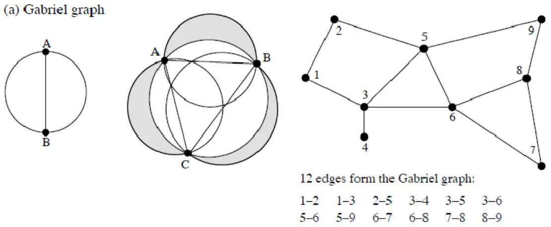
For the study of these situations, a very useful geometric connecting scheme is the Gabriel graph (Gabriel & Sokal, 1969).
With this criterion, the line connecting two points is part of the Gabriel graph if and only if no other point C lies inside the circle whose diameter is that line (Fig. 6).
In this way, starting from point A, it is possible to find all the points closest to it, with which it will be connected.
2.2.7. Ordination methods and Principal Coordinates Analysis
Matrices obtained with the different distance, dissimilarity or association indexes can be visully explored to identify the most similar samples. This, however, becomes particularly difficult, if not impossible, with a huge data set, which
Fig. 6. a) Left: geometric criterion for the Gabriel graph. Centre: the zone of exclusion of the criterion, here for three points (grey zones + white inner circle). Right: graph for the example data,
27
therefore generates an extremely large matrix: a typical situation in cases of a list of species observed in a certain number of samples.
In similar situations it is essential to use data analysis techniques, among which ordination methods are very useful. These have a dual purpose: to simplify the data set, reducing its dimensionality, defining linear combinations of its original variables preserving the information and to make a rigid rotation of the axes of the multidimensional space of data in a way to orient them in coherently with patterns of data dispersion.
The result is a graphical output, relatively simple to be interpreted, with the data being projected onto one or more planes, in which the Euclidean distance between the points representing the samples is proportional to the distance, dissimilarity or association value among them.
With this output a general comparison between the sites (or between the species, in the case of association index) is possible, in which the peculiarities of each station (or species) emerge.
As with the case of coefficients, even with ordination methods it is very important to choose the right technique, especially considering the starting data.
In this study Principal Coordinate Analysis (PCooA) (Gower, 1966), also called Metric Muldimensional Scaling (MDS) was used.
The algorithm on which the PCooA relies rotates and rescales the data set so that the distances in the resulting "cloud" are maximally correlated with the distances in the original data set. The optimal solution is found by calculating eigenvalues and eigenvectors through some steps:
The D matrix of distances, dissimilarities or association between the n objects
is transformed into the Δ matrix:
The Δ matrix is centered so that the origin of the axes system that will be defined is in the centroid of the objects. Thus the matrix C is obtained:
28
where the second and third terms represent the row and column averages of the Δ matrix and the last term represents the general average of the matrix.
Eigenvalues λj (j=1,2,...,m; m≤n-1) and eigenvectors uij (i=1,2,...,n; j=1,2,...,m)
of C matrix are calculated.
Principal Coordinates fij of the objects are obtained by multiplying the
eigenvectors by the square root of the corresponding eigenvalue:
The quality of the ordination obtained for each main axis can be assessed on the basis of the ratio between the corresponding eigenvalue and the sum of the extracted eigenvalues.
2.2.8. PERMANOVA
Permutational Multivariate Analysis of Variance (PERMANOVA) (Anderson, 2001a; Anderson, 2001b; McArdle & Anderson, 2001) is a non-parametric statistical test based on permutations, suitable for dealing with multivariate data. This test verifies whether the differences observed between two or more groups of objects, defined a priori by the researcher, are significant, starting from a dissimilarity/distance matrix calculated using any coefficient.
The F statistic is calculated as the ratio between the inter-group variance and the intra-group variance.
The null hypothesis of equal composition is rejected if the variability between the groups is significantly greater than that present within the groups themselves.
29
To test this, a p-value is assigned to the F statistic value, calculated with a random permutation process of the group elements, carried out for a sufficiently high number of times.
As in any other statistical test, the null hypothesis is formally rejected if p <0.05, or if the probability of randomly obtaining the same value of F or smaller ones is less than 5%.
2.2.9. Mantel Test
This test was originally developed for the study of the spatial distribution of occurrence of cancer cases (Mantel, 1967) and has recently been applied more and more often in the ecological field too.
It allows to obtain a measure of the degree of correlation between two matrices of distance, dissimilarity or association.
The null hypothesis tested is that of independence between the two matrices analyzed, while the probability level relative to the value of the statistic is calculated on the basis of an iterative procedure based on permutations of one of the two matrices.
The Mantel Z statistic, which expresses the degree of correlation between the structure of the two matrices, is calculated as the sum of the products of the corresponding elements of the two matrices, excluding those on the diagonal. It is also possible to calculate the Mantel statistics in a standardized form and in this case it is indicated with R, as in this work. The probability level associated with the Mantel statistic value is calculated, as already mentioned, on the basis of an iterative procedure that provides for the random permutation of the rows and columns of one of the two matrices and the recalculation of the Mantel statistic for a high number of times. The value of the statistic obtained for the original matrices is compared with the empirical distribution of those obtained by repeating the calculation on randomly permuted matrices: the percentage of iterations in which a value lower than the original one was obtained corresponds to the probability level of the latter. From a practical point of view the null
30
hypothesis of independence between the matrices will be rejected if less than 5% of the values obtained for the permuted matrices is higher than the original one.
2.2.10. Procrustes test (PROTEST)
Procrustes test is an alternative to Mantel test to relate data matrices.
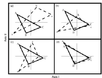
It is based on orthogonal Procrustes statistic (Hurley & Cattell, 1962), which combines together two ordination, derived from two different matrices with the same objects in rows. Each object has two representations. One of the data sets is kept fixed and the other one is rotated respect to the first, with a rotational-fit algorithm, with the aim of minimizing the sum of squared distances between the corresponding objects.
An example is shown in Fig. 7, where there are two triangles (X: A-B-C and Y: a-b-c) with different location, size and orientation.
X and Y are re-scaled and centered together (b). To make their orientation coincide, they are mirror reflected (c). Then. X is kept fixed and Y rotates until the sum of the squared distances between corresponding coordinates is minimized (d). In this way, the optimal superimposition is found.
The value of the squared distance (∆212) can be used as a measure of the
concordance between the two datasets. In fact, the lower ∆212 value is, the greater
the relation is.
Superimposition process requires that matrices have the same dimensions. This was not the case of our study, where we had two matrices with the same number
31
of rows (taxa), but a different number of columns (OSD). To overcome this obstacle, we reduced both sets to a two-dimensional space with the use of ordination technique to each matrix, as suggested by Peres-Neto and Jackson (2001).
As for the Mantel one, even Procrustes statistic can be tested to evaluate its significance. The test is called PROTEST (Jackson, 1995). In 2001, Peres-Neto and Jackson showed that PROTEST was more powerful than the Mantel test to identify correlations generated between raw data matrices.
The procedure is the following: Procrustes statistic is calculated;
rows are randomly permuted in relation to each other of one data matrix;
values for the permuted association are recalculated;
steps 2 and 3 are repeated a large number of times.
Smaller values of Prurustes statistic indicate higher concordance between data sets.
32
3. Results
As already said, this paragraph is divided into two subparagraphs, one for each objective of the Ph.D. project.
3.1. Predictive model for A. minutum occurrence
The study area is that of the NE Adriatic Sea, the species of interest is, as already mentioned, the dinoflagellates A. minutum. Species occurrence data were determined by PCR analysis performed on 187 surface seawater samples collected, monthly, from June 2005 to December 2009 along the transects of the Foglia and Metauro rivers at 500 m and 3000 m from coastland, by the Environmental Biology laboratory of the Department of Biomolecular Sciences of the University of Urbino. Information on environmental variables was obtained from the samples too, with laboratory analysis. The technique used is the RF. To select the combination of the different RF parameters that allowed us to get the best result, several RFs were trained. This multiple training was carried out in parallel for two different models: one trained using all the available environmental variables and one using only 12 out of the 18. The reduced data set excluded information about nutrients to make any future use of the model easier, with no need for water sampling and laboratory analysis to determine nutrients concentrations.
Results showed that 12-variables model was as good as the 18-variables one. In particular, the model is able to correctly predict more than 80% of the instances in the test data set. This underlines the important role that predictive models may play in the study of HABs.
Further information about experimental design and modeling procedure are given in the publication attached below.
33
3.2. OSD data analysis
For the second objective of the Ph.D. project, we analyzed the sequences of the encoding genes for the 18S rRNA of phytoplankton organisms found in seawater samples collected during the OSD campaigns in various areas of the world.
The dataset includes the list of different gene sequences present in each station. The assignment of a taxonomic identifier to the sequences has been possible up to the genus level for most of the records, while for the rest it has been possible to arrive at higher taxonomic levels.
The dataset contains both zoo- and phytoplankton, eukaryotic and prokaryotic species. For this work only the phytoplankton eukaryotic ones were considered, leaving the others aside.
First, a check was carried out on the original dataset, eliminating the ambiguous
taxa, or merging them at the higher taxonomic level where identification at a
lower level was not possible. Moreover, ubiquitous species (present in more than 80% of the stations) were eliminated. Stations with particular features (for example those of brackish water) were not taken into account, too.
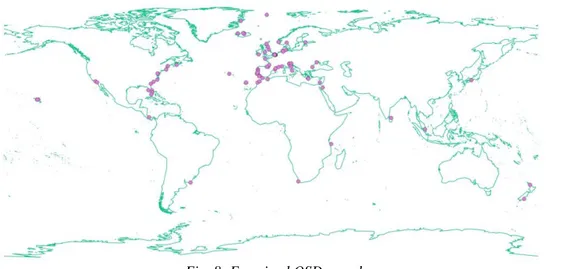
The dataset resulting from these first operations, on which the subsequent analysis were carried out, is composed of 103 stations and 187 different taxa (Fig. 8).
34
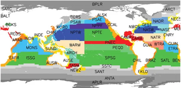
From a geographical point of view, marine environment can be divided into several ecoregions. Among the various classifications present in the literature, the one taken in support of our analysis is that of the biogeochemical provinces of Longhurst (1998) (Fig. 9).
Longhurst Province ID
Coastal - Brazil Current Coastal Province BRAZ Coastal - California Upwelling Coastal Province CCAL Coastal - Canary Coastal Province (EACB) CNRY
Coastal - E Africa Coastal Province EAFR
Coastal - Guianas Coastal Province GUIA
Coastal - NE Atlantic Shelves Province NECS Coastal - New Zealand Coastal Province NEWZ Coastal - NW Atlantic Shelves Province NWCS Coastal - Red Sea, Persian Gulf Province REDS Coastal - Sunda-Arafura Shelves Province SUND
Polar - Atlantic Arctic Province ARCT
Polar - Atlantic Subarctic Province SARC
Polar - Boreal Polar Province (POLR) BPLR
Trades - Caribbean Province CARB
Trades - Indian Monsoon Gyres Province MONS Trades - N. Pacific Tropical Gyre Province NPTG Westerlies - Kuroshio Current Province KURO Westerlies - Mediterranean Sea, Black Sea MEDI
Fig. 8: Examined OSD samples.
35 Tab. 2 shows names and
identification codes of the
different provinces
involved in our study.
Due to the denominations' length, reference will be made to the identification codes, in the text below.
Through PAST (PAleontological Statistics) program, developed by Hammer et al. (2001), a dissimilarity matrix was generated, taking the different stations as object and using the complement to 1 of the Jaccard coefficient.
Starting from this matrix, it was possible to explore the data through PCoA. The obtained ordination is shown in Fig. 10.
Province
Westerlies - N. Atlantic Subtropical Gyral Province (East) (STGE)
NASE Westerlies - S. Pacific Subtropical Gyre Province SPSG
36
Fig. 9: Longhurst biogeochemical provinces.
Fig. 10: Ordination obtained through Principal Coordinate Analysis of OSD samples. The ordination is based on Jaccard coefficient and the first two axes explain 19.4% of the total variance. Different colors
37
The first two principal axes respectively explain 11.3% and 8.14% of the total variance.
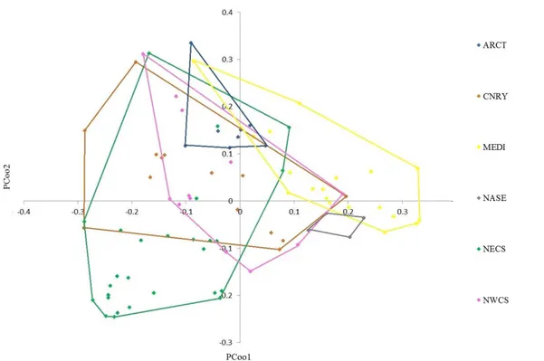
Each point is associated with an OSD and different colors correspond to different Longhurst ecoregions, listed in the legend. Overall, the points are uniformly arranged on the plane. Since some ecoregions are poorly represented, in Fig. 11 only those represented by at least four different stations are shown, with their convex hull.
The latter are almost all partially overlapping. This is true especially for provinces ARCT, CNRY, NECS and NWCS provinces. NASE is the most isolated of the six and this is probably due to the characteristic that distinguishes it from the others: together with NPTG, they are the only two, in the whole dataset, related to non-coastal waters and this could probably influence the phytoplankton composition present. The MEDI group is mainly placed on the first quadrant, with positive X
Fig. 11: Ordination of OSD samples belonging to Longhurst regions represented by at least four different stations, with their convex hull.
38
values and almost all positive Y values, with few exceptions. The ARCT group is mainly located in the second quadrant, with mainly negative X values and always positive Y values. The CNRY group focuses mainly on the second quadrant. The NWCS group is located in the center, covering all the four quadrants. The NECS group mainly occupies the third quadrant, the X values are almost all negative and so are those of the Y, with only a few exceptions. The NASE group is the only one to occupy only the fourth quadrant, with values of X always positive and Y always negative.
Looking at the X-axis, the main distinctions seem to exist between MEDI and CNRY, MEDI and NWCS and, above all, MEDI and NECS. In fact, all the points of the first, with the exception of one, are on the positive quadrants, while all the points of the second, except for two, are on the negative one. Looking at the Y axis, we can find again the distinction between MEDI and NECS and we also note that between NECS and NWCS.
In order to have a response that was not only exclusively visual, PERMANOVA was performed on the same matrix. Bonferroni corrected p-values are significant for almost all the couple of ecoregions considered (Tab. 3).
ARCT CNRY MEDI NASE NECS NWCS
ARCT 0.0136 0.0136 0.34 0.0136 0.1768 CNRY 0.0136 0.0136 0.3808 0.0136 0.8704 MEDI 0.0136 0.0136 0.0272 0.0136 0.0136 NASE 0.34 0.3808 0.0272 0.0136 0.0544 NECS 0.0136 0.0136 0.0136 0.0136 0.0136 NWCS 0.1768 0.8704 0.0136 0.0544 0.0136
Values highlighted in red do not allow to preserve the null hypothesis of equal composition of taxa in the different ecoregions, thus highlighting a difference in phytoplankton populations.
39
Later, a matrix of geographical connections between the various stations was created through an ad hoc program, starting from a Gabriel network. The obtained connections were modified where necessary, eliminating those that seemed unlikely, such as those linking OSDs separated from continental zones, and adding some, where it was known that there could be a connection between the OSDs, as in the case of Hawaiian stations linked to Japanese ones (Fig. 12).
With another ad hoc program, a space-constrained hierarchical clustering was carried out, with respect to the previously created connection matrix.
40
To determine which was the optimal number of clusters in which to divide the dataset, the mean intracluster distance was taken into account and, looking for the partition for which this value was lower (specifically, equivalent to 0.641), we were able to identify the one in 10 clusters as the most natural subdivision for the available data (Fig. 14 and 15) (legend in Tab. 4).
Most abundant clusters are B, which includes 33 stations, located in the North Sea and on the northern coasts of the Iberian peninsula and which fall within the space delimited by two Longhurst ecoregions (CNRY and NECS), A, with 16 stations exclusively present in the Mediterranean Sea (MEDI), C, with 12 stations, distributed on the Icelandic coasts and along the eastern coasts of Canada and northern United States (NWCS and ARCT) and D, the most heterogeneous among the groups, which includes 26 stations, located in various areas of the globe, which fall within 14 different ecoregions. That of group D can be considered a special case. In fact, looking at the map showed in Fig. 14 and 15, it can easily be
41
seen that these are much more numerous and close together in the northern hemisphere, while only 5 are found in the southern hemisphere.
These last samplings tend to be single spots, which have little in common with stations that are very distant from them. Therefore, the D group, in addition to the stations present along the eastern coast of the United States, groups all these individual cases, baing not very explanatory for the purposes of our analysis. The remaining 6 clusters are also special cases, which are
influenced by specific and localized
environmental conditions: E, with 3 stations, two on the west coast of the United States and one on
Fig. 15: Space-constrained clustering: detail of Italian stations.
Tab. 4: Clusters and relative colors on the map.
42
the Hawaiian Islands (CCAL and NPTG), F, with two stations in the Gulf of Venice (MEDI), G, with 5 stations along the southern coasts of the Iberian peninsula and Morocco (CNRY), H, with 3 stations in the Tagus estuary (CNRY), I, which includes the only station along the East African coast (EAFR) and J, with 2 stations in the Greenland Sea (ARCT and BPLR).
Given the nature of the available data, it was decided to focus the attention on the
two NECS and MEDI ecoregions. These include the 45% of the analyzed stations and therefore correspond to the area with the highest sampling density. This choice was also supported by the ordination results previously shown, in which the stations belonging to the two ecoregions are in distinctly separate groups on the plane. Furthermore, within this subset, only the stations belonging to clusters A and B have been taken into account, because the other represent those special
43
cases previously mentioned. Therefore, for the subsequent analyzes, 43 stations were considered, 16 belonging to group A and 27 to B (Fig. 16) and taxa absent in both stations have been eliminated from the dataset, keeping only 157 out of 187.
First, SIMPER analysis was carried out on the two groups of stations, to see which taxa contributes the most to determine the differences between the two ecoregions. Those responsible for 95% of these differences are 14. Specifically
Guinardia (29.06%), Rhizosolenia (22.09%), Alexandrium (16.85%),
Ostreococcus (6.73%), Heterocapsa (6.09 %), Bathycoccus (2%), Gymnodinium (1%), Protoperidinium (1%), Minutocellus (1%), Noctilucales (1%), Minidiscus (1%), with a greater number of reeds in group B, and Cyclotella (3.75%), Tetraselmis (2) and Halostylodinium (1%) with a greater number of reeds in group A.
Overall, 61.8% of taxa were present in both ecoregions, 22.9% in group B only and 15.3% in group A only.
Subsequently, the taxa frequencies in the two different groups of stations were compared, therefore the taxa present only in one of the two groups were eliminated from the dataset, keeping only that 61.8% present in both, so as to have two matrices with the same number of lines (objects) that could be matched. The number of taxa taken into account has therefore been reduced to 97.
To estimate the biodiversity of each station, starting from qualitative data, the percentage of taxa present compared to the total of those examined was taken
into consideration. The
result can be displayed in the box plot in Fig. 17.
44
Median values are close, but interquartile range is higher in group A then in group B.
Frequencies of the different taxa for the two different groups have been calculated
and reported in the graph in Fig. 18, where for every taxa there is a point, whose
coordinates are the frequency in group A on the X axis and that in group B on that of Y. Two proportion z-test was applied. Red point on the graph are taxa significantly more frequent in group B and blue points are significantly more frequent in group A.
Keeping the two groups separate, two association matrices between the different
taxa were created, based on the Fager & McGowan coefficient.
The two matrices were then compared to each other through Mantel test, to verify whether the tendency of certain taxa to appear together was linked to the region to which they belonged, or whether it was a more general trend. The result obtained (R = 0.4206 p = 0.0002) does not allow preserving the independence hypothesis,
Fig. 18: Frequency of taxa in group A (X axis) and group B (Y axis). Red point on the graph are taxa significantly more frequent in group B and blue points are significantly more
45
thus highlighting a certain correlation between the two matrices. This suggests an independence of the association from the geographical area to which it belongs.
Later, the two matrices were used as the basis for the same number of ordination via PCoA (Fig. 19 and 20).
Fig 19: Ordination obtained through Principal Coordinate Analysis of group A taxa. The ordination is based on the association matrix of Fager & McGowan and the first two axes explain 24.9% of the
46
PROTEST was used to compare the two ordinations, performed with R.
Results are shown in Fig. 21. Each arrow connects the two representations of each object (derived from the two different matrices). Arrow length provides information about the distance of the same object in the ordinations. Longer arrows correspond to greater distance, namely difference. As can be seen from the graph, values are all very small.
The null hypothesis of independent association matrices cannot be preserved, being the level of significance, p <0.0001. This result confirms what was previously obtained with Mantel test, and suggests that, even if there are differences in taxa associations between the two groups, they only concern a relatively small number of taxa and that overall relationships remain coherent, therefore independent of the belonging ecoregion.
Fig. 20: Ordination obtained through Principal Coordinate Analysis of group A taxa. The ordination is based on the association matrix of Fager & McGowan and the first two axes explain 20% of the