Contents lists available atScienceDirect
Journal of Multivariate Analysis
journal homepage:www.elsevier.com/locate/jmva
Describing the concentration of income populations by
functional principal component analysis on Lorenz curves
Enea G. Bongiorno
*, Aldo Goia
Dipartimento di Studi per l’Economia e l’Impresa, Università del Piemonte Orientale, via E. Perrone, 18 - 28100 Novara, Italy
a r t i c l e i n f o
Article history:
Received 12 August 2017 Available online 21 September 2018
AMS subject classification:
62H25 62F12 62P20
Keywords:
Consistency
Hanging cable problem Hilbert embedding approach Modes of variation
a b s t r a c t
Lorenz curves are widely used in economic studies (inequality, poverty, differentiation, etc.). From a model point of view, such curves can be seen as constrained functional data for which functional principal component analysis (FPCA) could be defined. Although statistically consistent, performing FPCA using the original data can lead to a suboptimal analysis from a mathematical and interpretation point of view. In fact, the family of Lorenz curves lacks very basic (e.g., vectorial) structures and, hence, must be treated with ad hoc methods. This work aims to provide a rigorous mathematical framework via an embedding approach to define a coherent FPCA for Lorenz curves. This approach is used to explore a functional dataset from the Bank of Italy income survey.
© 2018 Elsevier Inc. All rights reserved.
1. Introduction
In order to study the probability law of a random variable X , one can consider different real functions (provided their well-posedness), each one highlighting different aspects: the cumulative distribution function F and the corresponding density f or the quantile function, the quantile-density function, and the density-quantile function, respectively defined, for all p
∈
(0,
1), by Q (p)=
inf{
x:
F (x)≥
p}
, q(p)=
Q′(p)=
1/
f{
Q (p)}
and f{
Q (p)}
.An important aspect connected with the study of a distribution and that plays a key role in applied sciences (economics, biology, chemistry, etc.), is the notion of ‘‘concentration’’. Roughly speaking, it is the propension of a non-negative random variable X to redistribute over the individuals within the population. One of the goals in studying concentration is to characterize different settings ranging from the maximal concentration (one individual owns the total mass) and the equidistribution (the mass is distributed equally among all individuals).
In such a framework, a very useful tool is the so-called Lorenz Curve (LC) that was introduced in [27] to represent the concentration of wealth. Formally, given a non-negative random variable X with finite mean
µ
, its LC L(p) is defined, see [19], by L: [
0,
1] →
R:
p↦→
L(p)=
1µ
∫
p 0 Q (t)dt.
It is easy to see that L(0)
=
0, whereas L(1)=
1 as∫
Q (t)dt
=
µ
. Moreover, since Q (p) is non-negative and increasing, L(p) is increasing and convex.Because X
≥
0, the quantity∫
0pQ (t)dt may be interpreted as the mass of X held by the first 100×
p% of the individualsof a population ordered by increasing values of X , i.e., E
[
X 1{X≤Q (p)}]
, where 1Ais the indicator function of the set A, whereas*
Corresponding author.E-mail addresses:[email protected](E.G. Bongiorno),[email protected](A. Goia).
https://doi.org/10.1016/j.jmva.2018.09.005
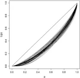
Fig. 1. Lorenz Curves of groups of individuals for class of age during the period 1987–2014.
µ
represents the total mass of X . Therefore, L(p) describes and measures how a positive quantity X concentrates within the population. From a mathematical point of view, the LC determines the probability distribution of X up to a scale factor transformation and uniquely characterizes the distribution whenever the latter has a known compact support; see, e.g., [24,35]. Among all LCs, the egalitarian line L(p)=
p plays an important role: it corresponds to a perfectly equaldistribution in which each individual owns the same quantity or when X is a degenerate random variable that equals
µ
. Any other LC lies below the equidistribution line that, hence, is used as a basis for comparison which leads to define concentration indexes measuring inequality within the population.Estimators of L(p) from samples drawn from X and their theoretical properties have been widely studied; see, e.g., [9–11,21,25,39].
Consider now the problem of comparing different distributions in terms of concentration: for instance to study the concentration of incomes over years, countries, regions, groups defined from social–economical stratification criteria, and so on. In all these situations, one deals with a set of estimated LCs, each one referred to a specific group. By way of example, the LCs computed from data gathered with the Survey on Household Income and Wealth of the Bank of Italy (see Section4 for details) are represented inFig. 1. Each curve graphs the concentration of personal income for individuals grouped for age range (up to 30 years old, 31–40, 41–50, 51–65 and over 65) and year of survey (from 1987 to 2014, biennial).
To manage that comparison problem, researchers focused on the construction of some hierarchies based on LCs. There exists a wide literature defining different kinds of orderings ranging from the use of synthetic indexes, like the Gini index, to stochastic orderings; see, e.g., [1,34] and references therein. The scientific debate on this topic, especially in the economic and econometric community, is still open, as testified by recent publications; see, e.g., the monographs [4,8] and references therein.
In this paper, the above mentioned problem is tackled for the first time, to our knowledge, using techniques from functional data analysis, which are designed for the analysis of data that are curves or more complicated objects such as images, surfaces, etc. To have an idea, although incomplete, of the wide variety of mathematical models, statistical techniques and feasible applications in such framework, see the collection of papers [3,5], the Special Issue [20], the survey [12] and the monographs [6,18,22,33].
To proceed in this direction, one needs a rigorous formal framework to fully exploit the functional nature of the data and to interpret the results meaningfully. A first difficulty stems from the fact that the considered functional data are not curves directly observed over a suitable grid, as it usually occurs in the classical functional literature, but a set of LCs, each one estimated from a sample of real random variables related to a specific level (a country, a region, and so on). This induces the necessity to manage a double stochasticity in the definition of the functional objects, a first one related to the sampling among the levels and a second one within each level.
Once the functional framework is rigorously defined, suitable statistical functional techniques can be used to identify structural properties and highlight differences among LCs. In particular, we focus on functional principal component analysis (FPCA), a technique which generalizes the well-known principal component analysis from finite- to infinite-dimensional spaces, and allows to reduce the dimensionality and to visualize the most important modes of variation of the data; see, e.g., [33]. This methodology requires that the data belong to a vector space, but the family of LCs cannot be straightforwardly endowed with a vector space structure since curves are non-negative, bounded, increasing and convex functions mapping
[
0,
1]
to itself. Hence, as we show in this paper, a naive direct application of FPCA is suboptimal because it could produce incoherent interpretations.In order to overcome this drawback, we propose to embed bijectively the family of LCs in a Hilbert space where FPCA results can be coherently interpreted. The bijection is derived in two steps. In the first step, each LC is seen as the unique solution of a boundary value problem whose physical interpretation allows to read the second derivative of each LC as a local inequality weight. In the second step, that second derivative is mapped to a Hilbert space through the negative centered log-ratio transformation. Although the latter map is often used in the compositional data literature, here we show that we deal with data that cannot be classified as compositional and, hence, the negative centered log-ratio transformation plays only a technical role. Besides the theoretical and algorithm aspects, we also study the consistency of the mode of variation of the FPCA obtained both in the naive and the embedding approaches.
To complete the analysis, the proposed method is applied to the study of the evolution of concentration of income of Italians from 1987 to 2014 using micro-data from the Survey on Household Income and Wealth of the Bank of Italy. After introducing three different stratification criteria (geographical, generational and sectorial), the method allows to analyze the positioning and the dynamic of each group, introduced by stratification, over time in the factorial plane.
Given the range of topics covered, this work can be thought as a new step forward in the study of samples of densities (see, e.g., [14,15,23,26,30,32]) and/or their derived objects such as level sets [16], quantile synchronized density [38] and hazard functions [32].
The outline of the paper is as follows. In Section2, we introduce the mathematical setting. In Section3, the naive FPCA approach on samples of LCs and the embedding one are introduced; their theoretical and algorithm aspects are then discussed. Finally, in Section4the methodology is applied to a real dataset. Proofs of the theoretical results are collected in theAppendix.
2. Lorenz curves as a functional data
This section introduces the mathematical aspects related to LCs as functional data. Consider a populationXformed by real and positive random variables X having probability density functions sharing the same compact support
[
0,
1]
and define the family of LCsLor
= {
L: [
0,
1] → [
0,
1] :
L(0)=
0,
L(1)=
1,
L∈
C2[
0,
1]
,
L′(p)
>
0 and L′′(p)
>
0 for p∈
(0,
1)}
.
BecauseLor is a subset ofL2[0,1], i.e., the Hilbert space of square integrable real functions on
[
0,
1]
with the inner product⟨
g,
h⟩ =
∫
g(t)h(t)dt and the induced norm∥
g∥
2= ⟨
g,
g⟩
,Lor can be endowed withBLor, theσ
-algebra induced by∥ · ∥
onL2[0,1]. On the populationXwe define the random LC as the map
L
:
(X,
BX)→
(Lor,
BLor):
X↦→
L(X )=
L(·
),
whereBX
= {
A⊆
X:
L(A)∈
BLor}
is theσ
-algebra induced by L, so that it is measurable. From now on and for the sake ofsimplicity, we will use L instead of L.
By considering L as a random element inL2[0,1], it is possible to define its mean curve and the covariance operator as
follows. For all p
∈ [
0,
1]
andv ∈
L2[0,1],ℓ
(p)=
E{
L(p)}
,
Σ(v
)=
E{⟨
L−
ℓ, v⟩
(L−
ℓ
)}
.
Consider now the empirical counterpart, and suppose we deal with a sample X1
, . . . ,
Xnof elements drawn fromX. To each Xiis associated an LC Liwhich, in practice, is estimated from a sample drawn from Xiof size ni, denoted Xi1, . . . ,
Xni
i . This can be done by introducing the empirical LC for the ith sample, defined for all p
∈ [
0,
1]
, byˆ
Li(p)=
1 Xi∫
p 0ˆ
Qi(t)dt,
(1)where Xiis the empirical mean and
ˆ
Qidenotes the ith empirical quantile function associated to Xi1, . . . ,
X nii . Consistency results for each empirical LC are available whenever Xiis absolutely continuous; see, e.g., [11]. Finally one has a sample of n functional data
ˆ
L1(p), . . . ,
ˆ
Ln(p). For computational purposes, each empirical LC can be evaluated over a common selected grid of points over[
0,
1]
.From estimator(1)one can define the empirical versions of the Lorenz mean curve
ℓ
and the covariance operatorΣby letting, for each p∈ [
0,
1]
andv ∈
L2[0,1],ˆ
ℓ
n(p)=
1 n n∑
i=1ˆ
Li(p),
Σˆ
n(v
)=
1 n n∑
i=1⟨
ˆ
Li−ˆ
ℓ
n, v⟩
(ˆ
Li−ˆ
ℓ
n).
Summarizing, this setting allows to model those situations in which a measurement (such as the income) concentrates in different regions or levels. In these cases, researchers deal with different empirical LCs, each one related to a different level. From a theoretical point of view, this means that one has to handle a double stochasticity: one related to the randomness of the distribution (between the levels) and the other linked to the sample variability (within the levels). In other words, a random unobserved distribution is associated to each individual (the level or the region) and, from such distribution, a sample is drawn to get the corresponding empirical LC.
3. Functional principal component analysis for Lorenz curves
In the previous section, LCs and their empirical counterparts are defined to fit the ‘‘classical’’ functional data analysis framework in which random functions are observed over a grid of deterministic points. We are now ready to tackle the problem of reasonably applying the FPCA to empirical LCs. In Section3.1we discuss how a naive use of FPCA could produce some incoherences. In Section3.2we present the embedding that is the starting point to perform FPCA whose results are coherent, interpretable and statistically consistent as shown in Section3.3.
3.1. Problems using a naive approach
SinceLor
⊂
L2[0,1], the latter seems a good candidate to implement FPCA in a naive way. Consider the eigenvaluesλ
1, λ
2, . . .
and eigenfunctionsξ
1, ξ
2, . . .
of the covariance operatorΣ. From them it is possible to approximate L by means ofa truncated version of the Karhunen–Loève decomposition of integer order q
≥
1; see Theorem 1.5 in [6]. For all p∈ [
0,
1]
,Lq(p)
=
ℓ
(p)+
q
∑
j=1
θ
jξ
j(p),
(2)where
θ
j= ⟨
L−
ℓ, ξ
j⟩
is the so-called jth principal component of L, satisfying E(θ
j)=
0, E(θ
j2)=
λ
jand E(θ
jθ
h)=
0 if j̸=
h. Because the eigenfunctionsξ
1, ξ
2, . . .
can also be seen as the result of a variance maximization iterative procedure, they arecommonly used to visualize the most important modes of variation of the random curve as perturbations of the mean. In practice, the jth modes of variation, defined, for all p
∈ [
0,
1]
and real k≥
0, byω
j(
p,
k) = ℓ ±
k(λ
j)1/2ξ
j(
p) ,
are interpreted as the effects of adding and subtracting a suitable multiple of each non standardized eigenfunction
√
λ
jξ
j. The constant k is usually chosen subjectively to better appreciate how the differentξ
js affect the mean.From the estimator(1)one can define the empirical versions of objects introduced above. In particular, once estimates (
ˆ
λ
1,n,
ˆ
ξ
1,n), . . . ,
(ˆ
λ
n,n,
ˆ
ξ
n,n) of the eigenelements (λ
1, ξ
1),
(λ
2, ξ
2), . . .
are derived from the eigendecomposition of theempir-ical covariance operator
ˆ
Σn, one can obtain the empirical versionˆ
Lq
i,nof(2), the empirical PCs
ˆ
θ
i,j,n= ⟨
ˆ
Li−ˆ
ℓ
n,ˆ
ξ
j,n⟩
, and the empirical jth modes of variation, given, for all p∈ [
0,
1]
and k≥
0, byˆ
ω
j,n(
p,
k) =
ˆ
ℓ
n(p)±
kˆ
ξ
j,n(p)(ˆ
λ
j,n)1/2.
For practical purposes, as empirical LCs are computed over a grid of finite points over
[
0,
1]
, all the calculations are made replacing integrals by summations.As a matter of completeness, it is useful to analyze the behavior of the estimated jth modes of variation when the sizes n and nidiverge. To do this and to manage the double stochasticity, we assume that a family
{
F (x, γ
)}
of random cumulative distribution function is associated to the populationX. The randomness depends on the real random vectorγ
and the following conditions are assumed:(A1) F (
γ , ·
) and F−1(γ , ·
) are a.s. continuous on[
0, ∞
) and (0,
1) respectively.(A2) There exists a positive constantΛindependent on
γ
, such that∫
∞0 x
2dF (
·
,
x)≤
Λ< ∞
a.s.(A3) There exist
δ >
0 and two positive constants c1and c2such that c1n2δ≤
ni≤
c2n2δas n→ ∞
.In this framework we derive the following consistency result whose proof can be found inAppendix A.3.
Proposition 1. Under Assumptions (A1)–(A3), for a fixed integer j
∈
N= {
1,
2, . . .}
and real k≥
0, one hasˆ
ω
j,n(p,
k)→
ω
j(p,
k) in probability, as n→ ∞
.At this stage, it is worth noticing that the Karhunen–Loève decomposition leads to approximations Lqand
ˆ
Lq
i,n, and modes of variations
ω
j(p,
k) andˆ
ω
j,n(p,
k) that are functions inL2
[0,1] but not necessarily inLor, as illustrated in the following
example.
Example 1. Consider L(p)
=
Upa+
(1−
U)pb, p∈ [
0,
1]
, with 1≤
a<
b, and U uniformly distributed on[
0,
1]
. The covariance operator has a unique eigenvalueλ =
1/
12 with associated eigenfunctionξ = |
pa−
pb|
. Direct calculations lead toω (
p,
k) =
(pa+
pb)/
2±
k(pa−
pb)/
√
12
,
which is aL2[0,1]function belonging toLor only for 0
≤
k<
√
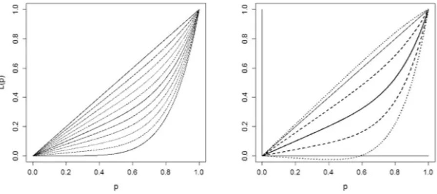
3. This is visualized inFig. 2where we have graphed a set of curves from L with a
=
1, b=
6 and selected values of U∈ {
0,
0.
1, . . . ,
1}
(left panel), and the corresponding modes of variation when k=
1 and k=
2 (right panel). It is evident that theω
(p,
1)s are elements ofLor whereas theω
(p,
2)s are not. Hence, the idea of using FPCA naively inLor, though it produces consistent estimates, suffers from drawbacks thatFig. 2. Left panel: a set of LCs with a=1, b=6 and U∈ {0,0.1, . . . ,1}. Right panel: the mean curve and the egalitarian line (solid lines), the modes of variation when k=1 (dashed lines) and k=2 (dotted lines).
ofL2[0,1], as can be verified straightforwardly. Thus, in what follows we consider a bijective continuous embedding for LCs that allows to represent them in a structured space and to apply FPCA to the transformed functions. It turns out that such embedding spontaneously induces a Hilbert space structure onLor.
3.2. An embedding approach
When one deals with a dataset of constrained functions (e.g., positive, and/or monotone, and so on), a typical approach to provide structured spaces, is to consider some transformations of the original data. In particular, it can be useful to express them as solutions of differential equations which often are related to physical interpretation; see [33].
The features of LCs suggest to draw inspiration from the so-called ‘‘hanging cable’’. Interpreting an LC L as a cable whose extremes are fixed at positions (0
,
0) and (1,
1) with linear density mass given by the second derivative L′′, the aim is to find the shape which minimizes its potential energy. In this perspective, L is the unique solution of the boundary value problem (BVP)
{
u′′(p)
=
L′′(p) if p∈
(0,
1),
u(0)
=
0,
u(1)=
1.
As shown inAppendix A.1, such a solution can be expressed, for all p
∈ [
0,
1]
, asL(p)
=
p+
(p−
1)∫
p 0 zL′′(z)dz+
p∫
1 p (z−
1)L′′(z)dz.
(3)The above representation provides a characterization of the LCs by means of their second derivative. This is summarized in the following commutative diagram:
Lor D2
→
←−
BVP D2Lor,
where D2Lor= {
L′′:
L
∈
Lor}
, D2 denotes the second derivative operator and BVP is the operator which, applied toan element in D2Lor, associates its BVP solution according to(3). It is worth noting that L′′
can be seen as the non-linear warped version of the probability density function f (x) given, for all p
∈
(0,
1), byL′′(p)
=
1/µ
f{
Q (p)} =
s(p)/µ,
(4)where f
{
Q (p)}
is called density-quantile (see [31]), and its reciprocal s(p) is known as the sparsity function; see [36]. Because s(p), and consequently L′′(p), measures the extent of sparseness of the data around the p-quantile, from the concentration point of view, L′′(p) can be also interpreted as a local measure of inequality of individuals close to the p-quantile. Summarizing, the physical interpretation of the hanging cable problem, together with(4), provides a new economic interpretation of L′′(p) as the local inequality weight at the p-quantile.The properties and the interpretation above move the attention to D2Lor, which is still not a vector space, as it contains
only non-negative functions. Nevertheless it is an important tool in developing further analysis. In fact, considerL2c
= {
g:
g
∈
L2[0,1], ∫
g=
0}
, the Hilbert space of centeredL2[0,1]-functions, and the negative centered log-ratio transformation nclr:
D2Lor→
L2c:
h↦→ −
ln(h)+
∫
1 0The latter embeds D2Lor inL2
cand its inverse function is nclr−1
:
L2c→
D2Lor:
g↦→
exp(−
g)/κ
g,
where
κ
g=
∫
1 0∫
p0exp
{−
g(z)}
dzdp. Hence, as shown inAppendix A.2, the following commutative diagram holds:D2Lor nclr
→
←−
nclr−1 L2c.
(6)Combining the above maps, we get the bijective transformation
ψ
(L)=
nclr(L′′) that associates each LC (having a square integrable log-second derivative) to an element of the Hilbert spaceL2
c. Its inverse is given by
ψ
−1(g)=
BVP{
exp(−
g) /κ
g
}
(7)for any centered square integrable function g. For the sake of readability, technical aspects concerning the invertibility of
ψ
are discussed inAppendix A.2.It is worth noting that the nclr transformation is often employed in the literature which generalizes compositional data (see [2]) to the continuous case in order to work in a proper Hilbert space. For instance, in [23] the authors consider the family of probability density functions; each one is a representative of the equivalence class containing all its positive multiples. One may thus wonder whether L′′
can be considered as a continuous compositional data, i.e., if any positive multiple of L′′
leads to the same LC by means of(3). In general it is not true: for instance, take the LC L(p)
=
p(p+
1)/
2 whose second derivative is L′′(p)
=
1 for all p∈
(0,
1) and consider cL′′, with c
>
2; Eq.(3)gives a function which is not even an LC because it is negative for p∈
(0,
1−
2/
c). The main difference between the compositional framework and our setting isrelated to the inversion of the nclr. Indeed, in the compositional setting, the inverse function is C exp(
−
g), where the positiveconstant C can be chosen arbitrarily, whereas in our setting, the constant must be
κ
gto guarantee the invertibility ofψ
; see Appendix A.2.To conclude this section, we provide some comments on the assumption that the considered random variables X have pdfs with common support
[
0,
1]
. Since each LC identifies the underlying pdf up to a scale factor, the proposed FPCA approach still holds if one takes[
0,
b]
, with 0<
b< ∞
, instead of[
0,
1]
. In contrast, if one takes[
a,
b]
, with 0<
a<
b< ∞
, thenψ
is no longer bijective. One possible solution is to work on the family of LCs obtained from X−
a keeping in mind that,although the LCs of X and X
−
a are different, they are related by an affine transformation whose known coefficients dependon a and the mean of X .
3.3. Computational aspects and consistency results
Consider the problem of estimating FPCA by using the embedding approach discussed above. Given a sample of empirical LCs
ˆ
L1(p), . . . ,
ˆ
Ln(p), as in Section2, one has to evaluate the second derivatives. Since eachˆ
Li(p) is linear piecewise, to work directly on it does not make sense: one possible solution is to obtain a smoothed version˜
Li(p) from which to derive˜
L′′
i(p). Various approaches are feasible for algorithmic purposes: for instance, one can use B-splines [13], constrained penalized splines [29], a suitable kernel smoothing approach [37], or local polynomial smoothing [17].
Once a sample of smooth curves
˜
L′′
1(p)
, . . . ,
˜
L′′
n(p) is available, each curve can be transformed by using the nclr map(5)to obtain, for each i
∈ {
1, . . . ,
n}
,ˆ
Ψi(p)= −
ln{
˜
L ′′ i(p)} +
∫
1 0 ln{
˜
L ′′ i(p)}
dp,
where the integral is evaluated numerically.Given Ψ
ˆ
1(p), . . . ,
Ψˆ
n(p), the empirical meanˆ
ψ
n, the covariance operator ΣΨ,ˆ
n and its eigenelements (ˆ
α
j,n,ˆ
ν
j,n) arecomputed. This allows to obtain a truncated reconstruction of order q, viz.
ˆ
Ψi,q(p)=
ˆ
ψ
n(p)+
q∑
j=1⟨
ˆ
ν
j,n,
Ψˆ
i⟩
ˆ
ν
j,n,
and the jth modes of variation,
ˆ
mj,n(k
,
p)=
ˆ
ψ
n(p)±
kˆ
ν
j,n(p)(ˆ
α
j,n)1/2
.
As usual in FPCA, the fraction of explained variance is computed from the eigenvalues
ˆ
α
j,n.To obtain the reconstructions of order q of Liand the jth modes of variation inLor[0,1], we apply the inverse transformation
(7)to
ˆ
Ψi,q(p) andˆ
mj,n(k,
p), respectively:ˆ
Li,q(p)=
p+
p−
1κ
Ψ∫
p 0 ze−ˆΨi,q(z)dz+
pκ
Ψ∫
1 p (z−
1)e−ˆΨi,q(z)dz,
ˆ
Mj(k,
p)=
p+
p−
1κ
m∫
p 0 ze−ˆmj,n(k,z)dz+
pκ
m∫
1 p (z−
1)e−ˆmj,n(k,z)dz,
Table 1
Some synthesis indicators for each age group during the time: Means and standard deviations of personal income (divided by 1000), and sample sizes.
Survey <30 31–40 41–50 51–65 >65
Year Mean Std. Size Mean Std. Size Mean Std. Size Mean Std. Size Mean Std. Size
1987 16.1 9.2 2004 22.9 13.6 2269 25.8 18.9 2248 22.5 19.3 3272 14.2 11.6 2468 1989 17.3 8.9 2525 24.5 14.7 2515 28.1 20.6 2561 24.0 20.0 3742 15.3 13.1 2465 1991 16.2 10.8 2159 23.0 13.8 2494 26.8 17.0 2596 23.3 18.5 3838 15.5 11.8 2777 1993 13.5 10.1 2070 21.5 15.7 2464 25.3 20.7 2500 23.2 21.9 3934 15.6 14.0 3305 1995 12.1 8.4 2135 20.0 15.2 2481 23.5 18.4 2650 23.0 25.2 3891 16.0 14.7 3341 1998 12.4 10.0 1785 20.8 17.0 2275 25.2 18.6 2404 24.4 25.1 3470 18.2 24.4 2682 2000 12.1 8.3 1896 20.7 18.0 2442 23.7 18.3 2655 24.2 22.4 3976 17.3 18.0 3333 2002 12.9 11.5 1592 20.0 14.1 2180 23.7 19.3 2559 23.5 21.1 3963 17.4 14.5 3724 2004 13.0 11.9 1524 20.7 25.5 2119 24.1 30.6 2495 24.0 22.9 3941 17.9 14.8 3827 2006 12.8 9.3 1355 20.6 28.2 1930 24.4 21.6 2494 24.4 23.4 3784 18.8 15.1 3851 2008 11.7 8.3 1344 18.0 10.9 1838 22.7 17.6 2545 24.3 21.2 3872 19.4 16.6 4074 2010 11.0 7.7 1230 17.6 11.3 1611 22.5 17.5 2622 24.5 20.3 4069 19.8 18.4 4152 2012 9.9 6.6 1042 16.0 9.7 1516 19.8 14.5 2462 22.5 18.4 4212 19.3 17.2 4377 2014 9.9 8.2 949 15.2 9.8 1271 19.5 15.2 2156 21.8 17.2 4190 18.9 13.9 4907 with
κ
Ψ=
∫
1 0∫
p 0 exp{−ˆ
Ψi,q(z)}
dzdp, κ
m=
∫
1 0∫
p 0 exp{−
ˆ
mj,n(k,
z)}
dzdp.
The integrals are computed as above.To conclude this section, we present the main consistency results on the jth modes of variation for a given positive integer
j when the smoothed curves
˜
Liare obtained by means of B-splines withτ
iequispaced knots andτ
i=
o(ni). In addition to assumptions (A1)–(A3) as in Section3.1, we also consider(A4) The pdf f belongs to F
= {
f:
suppf= [
0,
1]
,
f>
0, ∫
f=
1, ∫
f ln4f< ∞}
.Proposition 2. Under Assumptions (A1)–(A4), for a fixed integer j
≥
1 and real k≥
0, one has, as n→ ∞
,ˆ
mj,n(k,
p)→
mj(k,
p) andˆ
Mj,n(k,
p)→
Mj(k,
p) in probability, where mj(k,
p) and Mj(k,
p) are the theoretical jth modes of variation when LCs are observed integrally and not over samples.The proof ofProposition 2can be found inAppendix A.4. 4. Application to real data
Since 1965, the Bank of Italy conducts the Survey on Household Income and Wealth. From 1987 it is biennial and the collected data are comparable over time. The survey supplies information on income, saving, consumption expenditure and real wealth of Italian households, as well as anagraphic and labor aspects. The total sample size, in the most recent surveys, is about 8000 households, corresponding to about 20000 individuals.
Starting from the data of personal income in Italy from 1987 to 2014, appropriately adjusted for inflation, we estimated the LCs for specific groups of individuals. Among the available stratification criteria in the survey (geographical, socio-economic, cultural), we considered a demographic variable, the age of each income earner, which seems interesting in studying the generational gap. For this variable, five age-classes are available: 30 years old or less, 31–40, 41–50, 51–65, and over 65. With this choice, matching age group and survey year, we had a sample of n
=
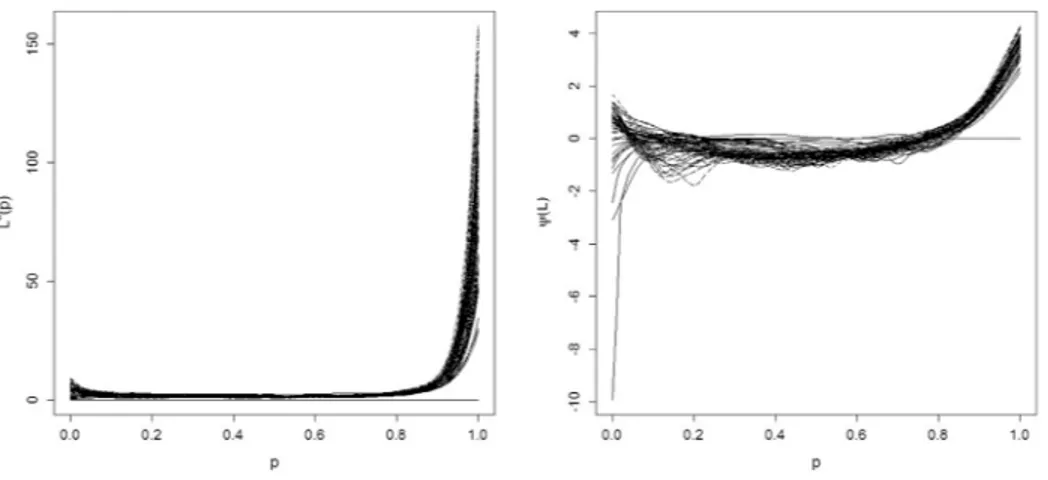
70 empirical LCs plotted in Fig. 1. Other details about the groups are collected inTable 1, where we report the mean and the standard deviation of income (for readability, they are divided by 1000) and the sample size.In order to apply the methodology illustrated in Section3.2, we need to estimate the second derivatives. Here we used a local polynomial smoothing approach, that, from our experience on data, seems to produce good results. In particular, we fitted a cubic polynomial with bandwidths computed according to the plug-in selector described in [17]. The shape of these functions is depicted inFig. 3.
By performing FPCA on the set of transformed dataΨ
ˆ
i, we estimated the PCs. The fractions of cumulative explained variance by the first three PCs are 0.553, 0.812, 0.884, respectively. In the left panel ofFig. 4the first three eigenfunctions of the empirical covariance operator in the transformed space are depicted. To illustrate how the first two eigenfunctions affect the shape of the LCs, we exhibit in the mid and right panels ofFig. 4the estimated modes of variation (in the original space)ˆ
Mj,n(k,
p) with j∈ {
1,
2}
and k= ±
3 (the dotted lines) and the theoretical LC obtained when k=
0 (the continuous line), that we denoteMˆ
n(0,
p).From the graphics, it transpires that the first eigenfunction takes its highest values close to zero, and relatively high values close to 1, whereas the values have opposite signs in the central part of the graphic. This suggests that the first eigenfunction describes the relationship between the weight of inequalities in correspondence to the extreme quantiles (in particular,
Fig. 3. Inequality weight functions (left) and transformed LC by means ofψ(right), of groups of individuals for class of age during the period 1987–2014.
Fig. 4. Left panel: First three eigenfunctions obtained performing FPCA inH. Mid and right panels: First and second modes of variation (the solid lines correspond to k=0, the dashed lines correspond to k= ±3).
left-quantiles) and the central ones. Thus, the scores of the first PC emphasize how the correspondent LCs behave near zero. In particular, the first PC opposes the LCs having almost horizontal tangent in a right-neighborhood of zero to those with a positive one. In other words, it seems that the first PC allows to distinguish groups where the first 10% of the individuals are very poor from the others, and this can be better appreciated by observing the shapes of the first modes of variation. As for the second eigenfunction, it seems to describe the curvature of LCs mainly due to a change of sign around p
=
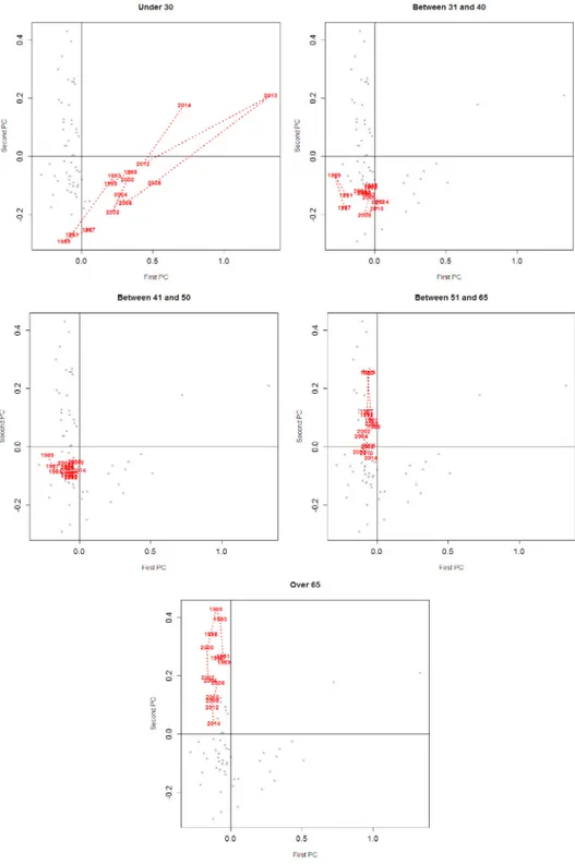
20%, and the level of the global concentration, i.e., the distance from the egalitarian line, in particular in correspondence of the central quantiles.To complete the analysis, we present the factorial plane based on the first two PCs. InFig. 5, we depict the track-plots associated to each age group. With respect to the first PC, the most significant result is a contrast between the group of under 30s and the other ones: the first ones exhibit a high inequality weight in the poorest part of the population and this aspect appears to have gotten worse over time. If we match this fact with the dynamic of the mean of income from 1987, and also consider the trend with respect to the second PC, it appears that the under 30s are becoming poorer (on average) with an ever stronger concentration at the expense of the poorest part of the population. A similar behavior, but with a moderate trend, can be found for people aged 41–50; also in these cases, one witnesses an (albeit less dramatic) impoverishment of the individuals and an increment of concentration. In fact, the tracks tend to converge toward the origin for the first PC, and this is a signal that the tangent of LCs close to zero becomes horizontal over time.
For what concerns the oldest part of the population, the most relevant movement is the vertical one (i.e., with respect the second PC). In these cases, the lines tend to converge toward the origin of the second PC: if the average of income appears rather steady over time (even tendentiously growing for the over 65), the LCs, which in the past denoted a better situation than the one described byM
ˆ
n(0,
p), tends more and more to look like the latter, denoting a worsening of the status of individuals in these groups.Fig. 5. Track-plots in the factorial plane of the first two PCs for different groups age.
Acknowledgments
The authors thank three anonymous referees, an Associate Editor, and the Editor-in-Chief for their valuable comments that allowed to improve the content and presentation of this paper. The authors are members of the Gruppo Nazionale per l’Analisi Matematica, la Probabilità e le loro Applicazioni (GNAMPA) of the Istituto Nazionale di Alta Matematica (INdAM).
The financial support of CRoNoS–COST Action IC1408 is acknowledged by the first author. The financial support of Università del Piemonte Orientale is acknowledged by the authors.
Appendix. Proofs
A.1. BVP solution
Consider the following BVP
{
u′′(p)
=
f (p) if p∈
(0,
1),
u(0)
=
0 if u(1)=
1,
and its general solutionu(p)
=
c1+
c2p+
∫
p 0∫
z 0 f (t)dtdz.
The boundary conditions lead to c1
=
0 and c2=
1−
∫
1 0∫
z0f (t)dtdz. By integration by parts, the latter can be rewritten as
c2
=
1+
∫
10(z
−
1)f (z)dz. Hence one hasu(p)
=
p{
1+
∫
1 0 (z−
1)f (z)dz}
+
∫
p 0∫
z 0 f (t)dtdzwhich, integrated by parts, leads to
u(p)
=
p+
p∫
1 0 (z−
1)f (z)dz+
∫
p 0 (p−
z)f (z)dzand, by straightforward calculation, to
u(p)
=
p+
(p−
1)∫
p 0 zf (z)dz+
p∫
1 p (z−
1)f (z)dz.
A.2. About the bijection
ψ
We prove that the function
ψ
is bijective and, as a by product, that the diagram(6)commutes. Thanks to standard results on bijective functions (see Chapter 1 in [28]), it is enough to show thatψ
−1{
ψ
(L)} =
L andψ{ψ
−1(g)} =
g for any g∈
L2c and L
∈ {
L∈
Lor,
ln L′′∈
L2[0,1]}
.Concerning the first equality, by Eq.(7), one has
ψ
−1{
ψ
(L)} =
BVP[
exp{−
ψ
(L)}
κ
ψ(L)]
,
whereκ
ψ(L)=
∫
1 0∫
p 0exp[−
ψ{
L(z)}]
dzdp. Explicitingψ
(L)=
ln L ′′−
∫
ln L′′and simplifying, one gets
ψ
−1{
ψ
(L)} =
BVP{
L′′∫
1 0∫
p 0 L ′′(z)dzdp}
which equals L because
∫
1 0∫
p0
L′′(z)dzdp
=
L(1)−
L(0)−
Q (0)=
1,
thanks to the definition of L, the fact that L′(p)
=
Q (p)/µ
and Q (0)=
0. Note that all the densities share[
0,
b]
as a common support.Concerning the second equality, by definition of
ψ
andψ
−1, one hasψ{ψ
−1(g)} = −
ln[
D2{
ψ
−1(g)}] +
∫
1 0 ln[
D2[
ψ
−1{
g(p)}]
]
dp= −
ln[
D2[
BVP{
exp(−
g)
κ
g}]]
+
∫
1 0 ln(
D2[
BVP[
exp{−
g(p)}
κ
g]])
dp.
Recalling that D2
{
BVP(g)} =
g, the result follows directly.A.3. Proof ofProposition 1
To prove that, as n
→ ∞
,ˆ
ω
j,n(k,
p)→
ω
j(k,
p) in probability for a fixed j and given k (we will drop k in the following expression), first observe that∥
ˆ
ω
j,n−
ω
j∥ ≤ ∥
ω
j,n−
ω
j∥ + ∥
ˆ
ω
j,n−
ω
j,n∥
.
(A.1)The result is obtained by showing that the two terms on the right-hand side of(A.1)tend to zero in probability as n
→ ∞
.First term. For the first summand on the right-hand side of(A.1), definitions and triangular inequalities lead to
∥
ω
j,n−
ω
j∥ = ∥
ℓ
n±
kξ
j,n(λ
j,n)1/2− {
ℓ ±
kξ
j(λ
j)1/2}∥
≤ ∥
ℓ
n−
ℓ∥ +
k{
(λ
j,n)1/2∥
ξ
j,n−
ξ
j∥ + ∥
ξ
j∥ × |
(λ
j,n)1/2−
(λ
j)1/2|}
,
(A.2) where, to avoid identification problems, we have supposed that⟨
ξ
j,n, ξ⟩
is positive, i.e.,ξ
j,nandξ
jpoint in the same direction. For the first summand in(A.2), the Strong Law of Large Numbers guarantees that for any p∈
(0,
1) and n→ ∞
,ℓ
n(p)→
ℓ
(p) in probability, and, sinceℓ
nandℓ
are bounded, then∥
ℓ
n−
ℓ∥
2→
0 in probability. Now consider the remaining terms in(A.2), viz.k
{
(λ
j,n)1/2∥
ξ
j,n−
ξ
j∥ + ∥
ξ
j∥ × |
(λ
j,n)1/2−
(λ
j)1/2|}
.
From now on, denote by C a universal positive constant. Using the fact that
∥
ξ
j∥ =
1,λ
1,n≥
λ
j,n, E(∥
ℓ∥
4)< ∞
(given by the boundedness of LCs), standard consistency results for the eigenelements (λ
j,n, λ
j,n) of the empirical covariance operator (see, e.g., Chapter 4 in [6]) apply and|
(λ
j,n)1/2−
(λ
j)1/2| ≤
C∥
Σn−
ΣL∥
∞, ∥ξ
j,n−
ξ
j∥ ≤
2√
2 min(λ
j−1−
λ
j, λ
j−
λ
j+1)∥
Σn−
ΣL∥
∞.
Hence, k{
(λ
j,n)1/2∥
ξ
j,n−
ξ
j∥ + ∥
ξ
j∥ × |
(λ
j,n)1/2−
(λ
j)1/2|} ≤
kC∥
Σn−
ΣL∥
∞and the right-hand side tends to 0 in probability as n
→ ∞
.Second term. Consider now the second summand in(A.1), i.e.,
∥
ˆ
ω
j,n−
ω
j,n∥
. As before, for fixed k and j, one has∥
ˆ
ω
j,n−
ω
j,n∥ ≤ ∥ˆ
ℓ
n−
ℓ
n∥ +
k{
(ˆ
λ
j,n)1/2∥ˆ
ξ
j,n−
ξ
j,n∥ + ∥
ˆ
ξ
j,n∥ × |
(ˆ
λ
j,n)1/2−
(λ
j,n)1/2|}
(A.3) and∥
ˆ
ℓ
n−
ℓ
n∥
2=
∫
1 0{
1 n n∑
i=1ˆ
Li(p)−
1 n n∑
i=1 Li(p)}
2 dp≤
1 n n∑
i=1∥
ˆ
Li−
Li∥
2.
In order to study the asymptotic behavior of
∥
ˆ
Li−
Li∥
, we fixγ = γ
0(the dependence onγ
0will appear when necessary)and assume (A1)–(A3). For each i, when ni
→ ∞
, the theorem on p. 114 in [11] states that there exists a positive and finite constant depending onγ
0, namely c(γ
0), such thatsup p∈[0,1]
|
(ˆ
Li−
Li)(α
0,
p)| ≤
c(γ
0)√
(ln ln ni)
/
ni a.s.
Using the same arguments as in the proof of Lemma 2.3 in [11], and thanks to Assumption (A2), we have c(
γ
0)≤
∫
∞ 0 x 2dF (γ
0,
x)≤
Λand∥
ˆ
Li−
Li∥ ≤
Λ√
(ln ln ni)/
ni a.s.
The latter, together with (A3), gives∥
ˆ
Li−
Li∥ ≤
c√
(ln ln ni)/
n2δ a.s.
(A.4) and 1 n n∑
i=1∥
ˆ
Li−
Li∥ →
0 a.s.,
(A.5)which guarantees that the first term in(A.3)vanishes as n
→ ∞
. Consider now the remaining terms in(A.3), i.e.,Given that (
ˆ
λ
j,n)1/2≤
(ˆ
λ
1,n)1/2a.s. and∥ˆ
ξ
j,n∥ =
1, (ˆ
λ
j,n)1/2∥
ˆ
ξ
j,n−
ξ
j,n∥ + ∥ˆ
ξ
j,n∥ × |
(ˆ
λ
j,n)1/2−
(λ
j,n)1/2| ≤
C∥ˆ
Σn−
Σn∥
∞,
where∥ˆ
Σn−
Σn∥
∞=
sup ∥v∥=1
1 n n∑
i=1{⟨
ˆ
Li−ˆ
ℓ
n, v⟩
(ˆ
Li−ˆ
ℓ
n)− ⟨
Li−
ℓ
n, v⟩
(Li−
ℓ
n)}
.
Note that⟨
ˆ
Li−ˆ
ℓ
n, v⟩
(ˆ
Li−ˆ
ℓ
n)− ⟨
Li−
ℓ
n, v⟩
(Li−
ℓ
n)= ⟨
ˆ
Li−ˆ
ℓ
n, v⟩
(ˆ
Li−
Li)+ ⟨
ˆ
Li−ˆ
ℓ
n, v⟩
(ℓ
n−ˆ
ℓ
n)+
+ ⟨
ˆ
Li−
Li, v⟩
(Li−
ℓ
n)+ ⟨
ℓ
n−ˆ
ℓ
n, v⟩
(Li−
ℓ
n).
The second and the fourth term sum to zero (due to the fact that the sum of the deviations from the mean is zero). Applying the triangular and Cauchy–Schwarz inequalities, and using the fact that
∥
v∥ =
1, we get∥
Σˆ
n−
Σn∥
∞≤
C n n∑
i=1 (∥
ˆ
Li−ˆ
ℓ
n∥ × ∥
ˆ
Li−
Li∥ + ∥
Li−
ℓ
n∥ × ∥
ˆ
Li−
Li∥
)≤
C n n∑
i=1∥
ˆ
Li−
Li∥
a.s.,
(A.6) where the last inequality holds because∥
ˆ
Li−ˆ
ℓ
n∥
and∥
Li−
ℓ
n∥
are almost surely bounded. Thank to(A.5), we get the desired conclusion. □A.4. Proof ofProposition 2
We have to prove that for a fixed integer j
∈
N and 0≤
k< ∞
, when n→ ∞
, one hasˆ
mj,n(k
,
p)→
mj(k,
p) in probability (A.7)and
ˆ
Mj,n(k
,
p)→
Mj(k,
p) in probability,
(A.8)which is equivalent to proving that, as n
→ ∞
,ψ
−1(ˆ
mj,n)
=
Mˆ
j,n(k,
p)→
ψ
−1(m
j,n)
=
Mj(k,
p) in probability. Given thatψ
−1(g)=
BVP{
exp(−
g)/κ
g
}
is continuous with respect to g,(A.8)is a consequence of(A.7)and thus we only prove(A.7).For a given k, by the triangular inequality, we have (dropping the dependence on k)
∥
ˆ
mj,n
−
mj∥ ≤ ∥
mj,n−
mj∥ + ∥
ˆ
mj,n−
mj,n∥
.
(A.9)The result is obtained by showing that the two terms on the right-hand side of(A.9)converge to zero in probability, as
n
→ ∞
.First term. For the first summand in(A.9), one has
∥
mj,n−
mj∥ = ∥
ψ
n±
kν
j,n(α
j,n)1/2− {
ψ ±
kν
j(α
j)1/2}∥
≤ ∥
ψ
n−
ψ∥ +
k{
(α
j,n)1/2∥
ν
j,n−
ν
j∥ + ∥
ν
j∥ × |
(α
j,n)1/2−
√α
j|}
,
(A.10) where, to avoid identification problems, we takeν
j,nsuch that⟨
ν
j,n, ν
j⟩
is positive.Concerning the first summand in(A.10), the Strong Law of Large Numbers guarantees that for any p
∈
(0,
1),ψ
n(p)→
ψ
(p) in probability as n→ ∞
. Thanks to Assumption (A4),ψ
n∈
L2[0,1](see technicalLemma 3, presented at the end of thisproof to improve readability) and thus, when n
→ ∞
,∥
ψ
n−
ψ∥
2→
0 in probability. Consider now the remaining terms of(A.10), viz.k
{
(α
j,n)1/2∥
ν
j,n−
ν
j∥ + ∥
ν
j∥ × |
(α
j,n)1/2−
(α
j)1/2|}
.
From now on, denote by C a universal positive constant. Using the fact that
∥
ν
j∥ =
1, andα
1,n≥
α
j,ntogether with standard consistency results for the eigenelements (α
j,n, ν
j,n) of the empirical covariance operator (see Chapter 4 in [6]), we have|
(α
j,n)1/2−
(α
j)1/2| ≤
C∥
ΣΨ,n−
ΣΨ∥
∞, ∥ν
j,n−
ν
j∥ ≤
2√
2 min(α
j−1−
α
j, α
j−
α
j+1)∥
ΣΨ,n−
ΣΨ∥
∞,
and, if E(∥
Ψ∥
4)< ∞
, as n→ ∞
,|
(α
j,n)1/2−
(α
j)1/2| →
0 and∥
ν
j,n−
ν
j∥ →
0 in probability.Hence, to prove the boundedness of the fourth moment, note that E(
∥
Ψ∥
4)=
E⎡
⎣
[
∫
1 0{
ln L′′(p)−
∫
1 0 ln L′′(
t)
dt}
2 dp]
2⎤
⎦
≤
4 E⎡
⎣
[
∫
1 0 ln2L′′(
p)
dp+
{∫
1 0 ln L′′(
t)
dt}
2]
2⎤
⎦
≤
16 E{∫
1 0 ln4L′′(
p)
dp}
=
16 E[
∫
1 0[
ln 1µ
f{
Q (p)}
]
4 dp]
≤
64ln4µ +
64 E[∫
1 0 ln4f{
Q(
p)}
dp]
=
C+
E[∫
1 0 ln4{
f(
x)}
f(
x)
dx]
< ∞,
where we have combined the definition, the Cauchy–Schwarz and Jensen inequalities, the substitution x
=
F−1(p) andAssumption (A4).
Second term. For the second summand of(A.9), one has
∥
ˆ
mj,n−
mj,n∥ = ∥ˆ
ψ
n+
kˆ
ν
j,n(ˆ
α
j,n) 1/2− {
ψ
n+
kν
j,n(α
j,n)1/2}∥
≤ ∥ˆ
ψ
n−
ψ
n∥ +
k{
(ˆ
α
j,n)1/2∥
ˆ
ν
j,n−
ν
j,n∥ + ∥
ν
j,n∥ × |
(ˆ
α
j,n) 1/2−
(α
j,n)1/2|}
.
(A.11) Consider∥ˆ
ψ
n−
ψ
n∥
. By the Cauchy–Schwarz inequality, the boundedness of the second derivatives and Lipschitz arguments, one can write∥ˆ
ψ
n−
ψ
n∥
2≤
4 n n∑
i=1∥
ln˜
L ′′ i−
ln L ′′ i∥
2≤
C n n∑
i=1∥
˜
L ′′ i−
L ′′ i∥
2.
Because
˜
Liis a smoothed version ofˆ
Li, then proving that∥
˜
L′′
i
−
L′′
i
∥ →
0 in probability, as ni(n)→ ∞
, guarantees that∥ˆ
ψ
n−
ψ
n∥ →
0 as n→ ∞
.Let Bi1
, . . . ,
Birbe a B-spline basis of degreeν ≥
2 andτ
iequispaced knots, ri=
ν + τ
i. Then˜
L ′′ i(p)=
ri∑
j=1˜
sijB ′′ ij(p),
where˜
si=
˜
b ⊤ i˜
C −1 i,
˜
C −1 i=
1 ni ni∑
j=1 Bi(pj)B ⊤ i (pj),
˜
bi=
1 ni ni∑
j=1 Bi(pj)ˆ
Li(pj)and Bi(p) being the B-spline vector. Moreover, denote by L
′′
i the smoothed version of L
′′ i, i.e., L′′i(p)
=
ri∑
j=1 sijB ′′ ij(p),
where si=
b ⊤ i˜
C −1 i and bi=
∑
nij=1Bi(pj)Li(pj)
/
niand consider the bound∥
˜
L ′′ i−
L ′′ i∥ ≤ ∥
˜
L ′′ i−
L ′′ i∥ + ∥
L ′′ i−
L ′′ i∥
.
(A.12)Concerning the first summand on the right-hand side of(A.12), note that
∥
˜
L ′′ i−
L ′′ i∥
2≤ ∥˜
b i−
bi∥
2× ∥
˜
C −1 i∥
2× ∥
G i∥
2,
where[
Gi]
ℓm=
∫
B′′iℓ(p)B′′im(p)dp. In view of the definitions of
˜
biand bi, and given(A.4), one has∥
˜
bi−
bi∥
2≤
C∥
ˆ
Li−
Li∥
2/τ
i≤
(Cn−i 2δln ln ni)/τ
i.
Using standard results on B-splines for functions observed on a regular discretization grid (see, e.g., Lemma 6.2 in [7]),
∥
˜
C−1
i
∥
2=
O(τ
−2
i ) and
∥
G∥
2=
O(τ
i3). Hence, when ni→ ∞
,∥
˜
L ′′ i−
L ′′ i∥
2=
O(n−2δ i ln ln ni) a.s.
(A.13)For the second summand on the right-hand side of(A.12), choosing
τ
i=
o(ni) and due to Lemma 6.2 in [7], one has∥
L′′i−
L′′i∥
2=
O(τ
i−4).
(A.14)Thus the bounds(A.13)and(A.14)guarantee that as n
→ ∞
,∥ˆ
ψ
n−
ψ
n∥ →
0 in probability. Consider now the remaining terms in(A.11):(
ˆ
α
j,n)1/2∥
ˆ
ν
j,n−
ν
j,n∥ ≤
(ˆ
α
1,n) 1/2∥
ˆ
ν
j,n−
ν
j,n∥ ≤
C∥ˆ
ΣΨ,ˆn−
ΣΨ,n∥
∞,
∥
ν
j,n∥ × |
(ˆ
α
j,n) 1/2−
(α
j,n)1/2| ≤
C∥ˆ
ΣΨ,n−
ΣΨ,n∥
∞,
whereˆ
ΣΨ,n[·] =
1 n n∑
i=1⟨ˆ
Ψi−
˜
ψ
n, ·⟩
(Ψˆ
i−
˜
ψ
n),
ΣΨ,n[·] =
1 n n∑
i=1⟨
Ψi−
ˆ
ψ
n, ·⟩
(Ψi−
ˆ
ψ
n).
Analogously to what was done to derive(A.6), one gets∥ˆ
ΣΨ,n−
ΣΨ,n∥
∞≤
C n n∑
i=1 (∥ˆ
Ψi−
ψ
ˆ
n∥ × ∥ˆ
Ψi−
Ψi∥ + ∥
Ψi−
ψ
n∥ × ∥ˆ
Ψi−
Ψi∥
)≤
C n n∑
i=1∥ˆ
Ψi−
Ψi∥
a.s.Since the fourth moment ofΨ is bounded, by using B-spline and similar arguments as above, one has
∥ˆ
Ψi−
Ψi∥
tends to zero in probability as n→ ∞
and thus∥ˆ
ΣΨ,n−
ΣΨ,n∥
∞→
0 in probability.Lemma 3. If (A4) holds, then
ψ
n∈
L2[0,1].Proof. By definition of
ψ
n(p) and applying the Cauchy–Schwarz inequality, we get∥
ψ
n∥
2=
∫
1 0{
1 n n∑
i=1 Ψi(p)}
2 dp≤
1 n2 n∑
i=1 n∫
1 0 Ψi(p)2dp=
1 n n∑
i=1
ln L′′ i(p)−
∫
1 0 ln L′′ i(
t)
dt
2≤
2 n n∑
i=1[
∥
ln L′′i(p)∥
2+
{∫
1 0 ln L′′i(
t)
dt}
2]
.
Thanks to Jensen’s inequality,
{∫
1 0 ln L′′i(
t)
dt}
2≤
∫
1 0{
ln L′′i(t)}
2dt and, thanks to(4),∥
ψ
n∥
2≤
4 n n∑
i=1∫
1 0{
ln L′′i(
t)}
2dt=
4 n n∑
i=1∫
1 0[
ln 1µ
ifi{
Qi(
p)}
]
2 dp=
4 n n∑
i=1 ln2µ
i+
4 n n∑
i=1∫
1 0 ln2fi{
Qi(p)}
dp.
For each i∈ {
1, . . . ,
n}
, substitute x=
Fi−1(p) to get∥
ψ
n∥
2≤
C+
4 n n∑
i=1∫
1 0 fi(
x)
ln2fi(x)dxwhich is finite, thanks to (A4). This concludes the proof. □
References
[1] R. Aaberge, Ranking intersecting Lorenz curves, Soc. Choice Welf. 33 (2009) 235–259.
[2] J. Aitchison, The Statistical Analysis of Compositional Data, Chapman & Hall, London, 1986.
[3] G. Aneiros, E.G. Bongiorno, R. Cao, P. Vieu, Functional Statistics and Related Fields, Springer, Berlin, 2017.
[4] G. Betti, A. Lemmi, Advances on Income Inequality and Concentration Measures, Routledge, London, 2008.
[5] E.G. Bongiorno, A. Goia, E. Salinelli, P. Vieu, Contributions in Infinite-Dimensional Statistics and Related Topics, Esculapio, Bologna, 2014.
[6] D. Bosq, Linear Processes in Function Spaces, Springer, New York, 2000.
[7] H. Cardot, Nonparametric estimation of smoothed principal components analysis of sampled noisy functions, J. Nonparametr. Stat. 12 (2000) 503–538.