Target tracking in marine environment from X-Band radar data

(1)

(2)

Finito di stampare nel mese di Febbraio 2016

Edizione

Collana Quaderni del Dottorato di Ricerca in Ingegneria dell’Informazione Curatore Prof. Claudio De Capua

ISBN 978-88-99352-02-8

Università degli Studi Mediterranea di Reggio Calabria Salita Melissari, Feo di Vito, Reggio Calabria

(3)

DANIELE ARTURI

TARGET TRACKING IN MARINE ENVIRONMENT

FROM X-BAND RADAR DATA

(4)

4

The Teaching Staff of the PhD course in

INFORMATION ENGINEERING

consists of:

Claudio DE CAPUA (coordinator) Raffaele ALBANESE Giovanni ANGIULLI Giuseppe ARANITI Francesco BUCCAFURRI Giacomo CAPIZZI Rosario CARBONE Riccardo CAROTENUTO Salvatore COCO Mariantonia COTRONEI Lorenzo CROCCO Francesco DELLA CORTE Lubomir DOBOS Fabio FILIANOTI Domenico GATTUSO Sofia GIUFFRE' Giovanna IDONE Antonio IERA Tommaso ISERNIA Fabio LA FORESTA Gianluca LAX Aime' LAY EKUAKILLE Giovanni LEONE Massimiliano MATTEI Antonella MOLINARO Andrea MORABITO Carlo MORABITO Giuseppe MUSOLINO Roberta NIPOTI Fortunato PEZZIMENTI Nadia POSTORINO Ivo RENDINA Francesco RICCIARDELLI Domenico ROSACI Giuseppe RUGGERI Francesco RUSSO Giuseppe SARNE’ Valerio SCORDAMAGLIA Domenico URSINO Mario VERSACI Antonino VITETTA

(5)

v

(6)

(7)

vii

List of Figures

Fig. 1.1 Basic principle of radar ... 4

Fig. 1.2 Mathematical view of state estimation ... 7

Fig. 1.3 Block diagram of target state estimation ... 8

Fig. 1.4 Optimal estimator issues ... 9

Fig. 1.5 Validation gate... 10

Fig. 2.1 Single target in clutter ... 15

Fig. 2.2 Multiple targets in clutter ... 17

Fig. 2.3 Main tracking algorithms ... 18

Fig. 2.4 State estimation system (part 1) ... 20

Fig. 2.5 State estimation system (part 2) ... 21

Fig. 2.6 Kalman filter feedback control ... 22

Fig. 2.7 NNSKF Functionality... 22

Fig. 2.8 PDAF Functionality ... 24

Fig. 2.9 Typical MTT system ... 29

Fig. 2.10 Association ambiguity ... 30

Fig. 2.11 General functionality of IMM ... 31

Fig. 3.1 Sea clutter origin (v, wind direction) ... 35

Fig. 3.2 Binomial distribution of false alarms ... 36

Fig. 3.3 False alarms distribution in function of their spatial density ... 37

Fig. 3.4a Single target without clutter (acquisition time t1) ... 38

Fig. 3.5b Single target without clutter (acquisition time t2) ... 39

Fig. 3.6c Single target without clutter (acquisition time t3) ... 39

Fig. 3.7a Single target with clutter assuming 3 false alarms every time instant tracked with NNSKF (acquisition time t1) ... 41

Fig. 3.8b Single target with clutter assuming 3 false alarms every time instant tracked with NNSKF (acquisition time t2) ... 41

Fig. 3.9c Single target with clutter assuming 3 false alarms every time instant tracked with NNSKF (acquisition time t3) ... 42

Fig. 3.10a Single target with clutter assuming 10 false alarms every time instant tracked with NNSKF (acquisition time t1) ... 42

Fig. 3.11b Single target with clutter assuming 10 false alarms every time instant tracked with NNSKF (acquisition time t2) ... 43

Fig. 3.12c Single target with clutter assuming 10 false alarms every time instant tracked with NNSKF (acquisition time t3) ... 43

Fig. 3.13a Single target with clutter assuming 3 false alarms every time instant tracked with Cheap PDAF (acquisition time t1) ... 44

Fig. 3.14b Single target with clutter assuming 3 false alarms every time instant tracked with Cheap PDAF (acquisition time t2) ... 45

Fig. 3.15c Single target with clutter assuming 3 false alarms every time instant tracked with Cheap PDAF (acquisition time t3) ... 45

Fig. 3.16a Single target with clutter assuming 10 false alarms every time instant tracked with Cheap PDAF (acquisition time t1) ... 46

Fig. 3.17b Single target with clutter assuming 10 false alarms every time instant tracked with Cheap PDAF (acquisition time t2) ... 46

(10)

List of Figures

x

Fig. 3.18c Single target with clutter assuming 10 false alarms every time instant tracked with Cheap PDAF (acquisition time t3) ... 47 Fig. 3.19a Two targets with clutter assuming 3 false alarms every time instant

tracked with NNSKF (acquisition time t1) ... 48 Fig. 3.20b Two targets with clutter assuming 3 false alarms every time instant

tracked with NNSKF (acquisition time t2) ... 48 Fig. 3.21c Two targets with clutter assuming 3 false alarms every time instant

tracked with NNSKF (acquisition time t3) ... 49 Fig. 3.22a Two targets with clutter assuming 10 false alarms every time instant

tracked with NNSKF (acquisition time t1) ... 50 Fig. 3.23b Two targets with clutter assuming 10 false alarms every time instant

tracked with NNSKF (acquisition time t2) ... 50 Fig. 3.24c Two targets with clutter assuming 10 false alarms every time instant

tracked with NNSKF (acquisition time t3) ... 51 Fig. 3.25a Two targets with clutter assuming 3 false alarms every time instant

tracked with Cheap JPDAF (acquisition time t1) ... 51 Fig. 3.26b Two targets with clutter assuming 3 false alarms every time instant

tracked with Cheap JPDAF (acquisition time t2) ... 52 Fig. 3.27c Two targets with clutter assuming 3 false alarms every time instant

tracked with Cheap JPDAF (acquisition time t3) ... 52 Fig. 3.28a Two targets with clutter assuming 10 false alarms every time instant

tracked with Cheap JPDAF (acquisition time t1) ... 53 Fig. 3.29b Two targets with clutter assuming 10 false alarms every time instant

tracked with Cheap JPDAF (acquisition time t2) ... 54 Fig. 3.30c Two targets with clutter assuming 10 false alarms every time instant

tracked with Cheap JPDAF (acquisition time t3) ... 54 Fig. 4.1 Architecture of the acquisition and processing system of the radar

data ... 58 Fig. 4.2 Installation site of the Remocean system indicated by the red circle 59 Fig. 4.3 Radar image showing clutter and moving targets at the port of Giglio

Island ... 60 Fig. 4.4 Radar image with three targets indicated by the red circles ... 60 Fig. 4.5 Block diagram of a detection and tracking system ... 61 Fig. 4.6 Pdf of the K-distribution for =1 and (blue),

(violet) and (yellow) ... 64 Fig. 4.7a Real data acquired by the X-band radar system tracked with NNSKF

(acquisition time t1) ... 65 Fig. 4.7b Real data acquired by the X-band radar system tracked with NNSKF

(acquisition time t2) ... 65 Fig. 4.7c Real data acquired by the X-band radar system tracked with NNSKF

(acquisition time t3) ... 66 Fig. 4.7d Real data acquired by the X-band radar system tracked with NNSKF

(acquisition time t4) ... 66 Fig. 4.8a Real data acquired by the X-band radar system tracked with Cheap

PDAF (acquisition time t1) ... 67 Fig. 4.8b Real data acquired by the X-band radar system tracked with Cheap

PDAF (acquisition time t2) ... 67 Fig. 4.8c Real data acquired by the X-band radar system tracked with Cheap

(11)

List of Figures

xi Fig. 4.8d Real data acquired by the X-band radar system tracked with Cheap

PDAF (acquisition time t4) ... 68 Fig. 4.9a Real data acquired by the X-band radar system tracked with Cheap

JPDAF (acquisition time t1) ... 69 Fig. 4.9b Real data acquired by the X-band radar system tracked with Cheap

JPDAF (acquisition time t2) ... 69 Fig. 4.9c Real data acquired by the X-band radar system tracked with Cheap

JPDAF (acquisition time t3) ... 70 Fig. 4.9d Real data acquired by the X-band radar system tracked with Cheap

(12)

(13)

xiii

List of Tables

Tab. 1.1 Frequency band in the range of microwaves... 5

Tab. 3.1 Main parameters ... 33

Tab. 4.1 Parameters of the acquisition system ... 57

(14)

(15)

1

Introduction

Radar surveillance applications are essentially based on target detection and tracking techniques, which are classic radar problems [1]. The aim is to provide the coordinates, the speed, the course and the behavior of a moving target or, in other words, to "follow" a target that moves along the sea surface. To this end, in the initial stage, the radar must detect the presence of the target within the scene under observation, through the so-called identification or detection procedure. Then, the tracking procedure is based on the analysis of a set of detection measures, associated with the same target, carried out at different time instants. Therefore, tracking is closely related to detection, so that a proper tracking must take into account all the problems connected with detection [2].

In a given instant of time, the radar provides a set of measures that may come from the target of interest, may be due to false alarms or clutter, or may have been generated from other targets. After the detection procedure, only the measures that come from the target of interest in the following time instants are considered, thus, defining the tracking of that target, namely the set of its positions in time. Consequently, given the set of all positions of a target up to the current time, it is possible to "predict" the position in the next measurement associated with that target [3].

During the tracking procedure, measurements that come from a target are processed in order to obtain an estimate of its current state [4], which typically consist of:

• Kinematic components — position, velocity, acceleration, turn rate, etc.

• Feature components — radiated signal strength, spectral characteristics, radar cross-section, target classification, etc.

(16)

1 Introduction

2

Target detection strategies aim to distinguish the radar echo of the electromagnetic return of a target from the unwanted signal (noise), which can affect the detection performances [5]. Obviously, in a multi-target scenario, it is more difficult to establish that the measurement received by the radar is originated from a particular target and, in addition to this, the output of a detection algorithm is characterized by the presence of false alarms, which can be interpreted as measurement noise and further complicate the target state estimate [6].

In marine environment, target tracking has a specific methodological interest, because it requires dealing with the peculiar problems related to the separation of useful signal from clutter signal, which can induce false alarms and ultimately lead to the loss of the target [7]. These issues, of course, call for proper solution procedures to address the classic problems of target tracking, namely the correct detection of targets and the association procedure, needed to determine which one of the detected signals has been originated by the target of interest [8]-[12].

The primary objective of target tracking is to estimate the state trajectories of a target. In the case of target moving on the sea surface, the main problems are:

 clutter, due to the presence of the capillary waves generated by the wind;

 target model uncertainties, due to the unexpected maneuver of the ship;

 measurement uncertainties, due to the presence of environmental and instrumental noise

X-band radar systems are used in a great variety of civil and military problems applications, weather monitoring and vessel traffic control. As regards applications in marine environment, they are considered a flexible and low-cost tool for ship detection and have attracted a growing interest in last decade, thanks to their capability of scanning the sea surface with high

(17)

1 Introduction

3 temporal and spatial resolution, their cost-effectiveness, as well as their simplicity of operation and installation [13]. However, in spite of their versatility, incoherent X-band radars are mostly employed for high resolution surveillance purposes but, in these scenarios, they cannot be considered as reliable as coherent systems in terms of target detection capabilities, with a consequent limitation in terms of target tracking. This is due to the fact that the result of a processing based only on the amplitude of the received signal that can be compromised by the presence of sea clutter, conversely coherent systems, by measuring both the amplitude of the signal received and its phase, can be more accurate. However, the employment of an effective tracking strategy can play a fundamental role in these circumstances, leading to a significant improvement in the surveillance performances provided by such coherent radar systems.

The thesis is organized as follows. Chapter 1 provides a study of the problematic of the identification and tracking of a moving target and the association procedure. Chapter 2 deals with some tracking problems and offers an overview of the principal tracking algorithms. Chapter 3 presents the validation and implementation of some of these algorithms on simulated data, including a description of the false alarm distribution. Chapter 4 presents the validation and implementation of some of these algorithms on real data acquired by an X-band radar installed at the port of the Giglio island, including a description of the clutter distribution. Chapter 5 presents the conclusions and the future perspectives.

(18)

1 Introduction

4

1.1 Introduction on RADAR principles

The term RADAR indicates an electronic apparatus used to detect the presence and measure of the position of objects (targets) by means of radio waves. This measure consists in determining the distance and the direction of objects from the radar, analyzing the signal backscattered by the target [14]. The operation of a radar is very simple: the same antenna transmits a signal and receives the echo due to reflections on possible obstacles, i.e., the targets. The distance is determined by measuring the time interval that elapses between the transmission and reception of the pulses, being known the speed of propagation of radio waves:

(1.1) (it must be considered the time of go and return of the signal).

If the transmitted pulses do not encounter any obstacle during their propagation, then they do not return back, that is, the signal travels unperturbed and it will be attenuated as the distance increases, while, in the case in which the beam hits an object, the signal is reflected and an echo is revealed from the receiver antenna [15] (Fig. 1.1).

(19)

1 Introduction

5 The type of electromagnetic radiations emitted by radar antennas are located within the microwave range. Following World War II, there is a classification of the electromagnetic radiation type according to different regions of wavelength:

Band Frequency (Ghz) Wavelength (cm)

P 0.225 - 0.39 77 - 133 L 0.39 – 1.55 19 - 77 S 1.55 – 3.90 7.7 – 19 C 3.90 – 6.20 4.8 – 7.7 X 5.75 – 10.9 2.8 – 5.2 Ku 10.9 – 18.0 1.7 – 2.8 Ka 18.0 – 36.0 0.8 – 1.7

Tab. 1.1 Frequency band in the range of microwaves

1.2 Radar properties

The operation of the radar is characterized by the following properties [16]:

Sensitivity refers to the ability of the radar to detect the reflected signal also

from weak targets. Normally, it is taken as the minimum input signal required to produce a specified output signal and it represents a measure of the interference generated by the radar (self-noise) against the minimum signal it is able to detect.

The measurements of the distance from the target is inherent in the name radar. The modern radar systems are capable of measuring the position of the target in a three dimensional space, its velocity vector and the angular direction of the vector of the angular speed and all these measurements may be made on more targets of interest with the presence of clutter and noise. The most advanced radar have also the ability to measure the extent, the shape and the classification of the target (person, building, airplane, etc.).

(20)

1 Introduction

6

The resolution corresponds to the ability of the radar to locate the desired target and distinguish it from the noise and clutter. In practice, there is a limitation in the resolution achievable due to the characteristics of the signal and the antenna. In particular, as regards the limitation in the resolution, it can be observed that a greater bandwidth provides better resolution in range, while a longer pulse durations allow improving frequency resolution.

Radar resolution is formally expressed by two figures: resolution in range and resolution in azimuth.

1. Resolution in range is the minimum distance that must exist between two objects such that the system is able to discriminate them, otherwise they become indistinguishable. It is defined as

2 min  c r   , (1.2) where c is the speed of light and τ it is the pulse duration.

2. Resolution in azimuth is the ability of radar equipment to separate two reflectors at similar ranges but different bearings from a reference point. It is defined as

D





 (1.3)

The expression is valid for large distances, where λ is the wavelength of the signal and D is the effective diameter of the antenna.

(21)

1 Introduction

7

1.3 Target tracking as an estimation problem

Estimation is the process of inferring the value of a quantity of interest from indirect, inaccurate and uncertain observations [17]. The variable of interest in an estimation problem can be:

 a parameter — a time-invariant quantity (a scalar, a vector or a matrix);

 the state of a dynamic system (usually a vector).

In this context, tracking procedures can be viewed as the estimation of the

state of a moving object.

The block diagram in Fig. 1.2 represents a general conceptual representation of the state estimation problem.

Fig. 1.2 Mathematical view of state estimation

There is no possibility to access to variables inside the dynamic and measurement systems, therefore the only variables which are available to the estimator are the measurements, which are obviously affected by the error sources modeled in the form of “noise.”

An optimal estimator is a computational algorithm that processes

observations (measurements) to yield an estimate of a variable of interest, that minimizes a certain error criterion.

As a consequence:

 the advantage of an optimal estimator is that it exploits the data and the knowledge of the system and of the noise in the best possible way (through a proper model);

(22)

1 Introduction

8

 the disadvantages are that it is sensitive to modeling errors and might be computationally expensive.

The block diagram in Fig. 1.3 is an extended version of the one in Fig. 1.2, which explains more in detail the conceptual representation of the dynamic system where detection and tracking are operating, the measurement system used to acquire data and the state estimator used to produce the results.

Fig. 1.3 Block diagram of target state estimation

The correspondences with the block diagram in Fig. 1.2 are the following:

 the block “Environment” refers to the block “Dynamic system”;

 the blocks “Sensor” and “Signal Processor” refer to the block “Measurement system”;

 the block “Information Processor” refers to the block “State estimator”.

Active sensors, like radars, emit energy into the environment and search for reflected energy. The backscattered signal is then processed by the signal processor and there is a measure. The measurements of interest are not raw data points but usually the outputs of complex signal processing and detection subsystems. Finally, the measurement is processed in order to obtain the target state estimate.

However, many problems can arise in a target detection and tracking procedure, as illustrated in Fig. 1.4. These problems can seriously affect the detection and tracking procedure and eventually compromise the outcome of the target state estimate.

(23)

1 Introduction

9

Fig. 1.4 Optimal estimator issues

As shown in the central part of the figure, the first two problems to take into account are:

 the number of sensors used to perform the tracking procedure, since a

single-sensor or a multi-sensor tracking procedure can be performed, considering that adding additional sensors to the observation system can produce a more accurate estimate of the trajectory, even though the multi-sensor tracking is subject to other issues to face;

 the number of targets to be tracked, which is a not well defined number.

Obviously, it is more difficult to track more targets all together and at the same time, because, if the system parameters are not properly defined, the signal of a target can produce interference to the signal of another target.

The right side of the figure shows the following problems:

 track stage, in particular the track formation (or initiation), it means

when the target is “seen” for the first time, and the track maintenance (or continuation), that is the ability to continue to follow the same target, a complex operation due to the presence of the false alarms because they can affect the tracking procedure;

(24)

1 Introduction

10

 if the target behavior is stationary or no stationary, that is if the movement of the target is subject to maneuvering or not, because in the no stationary case the target can suddenly change its trajectory possibly compromising its estimate.

Finally, the right side of the figure shows the problems of defining the:

 Sensor detection characteristics, that is Probability of Detection (PD) and

Probability of False Alarms (PFA), which are parameters used during the detection and tracking procedure that must be carefully evaluated in order to obtain a correct target trajectory estimate;

 Target size, that is if the dimension of the target is comparable to the

sensor resolution cell or if the target image is an extended one; the second case is more complex to deal with because the target signal received by the system is actually composed of a cloud of points.

1.4 The association problem and the validation region

Let us suppose that the set of all the positions occupied by the target up to the current time k-1 is known. Then, one can "predict" the position where it is more probable to find the next measurement associated with that target at instant k. The new measures provided by the radar will be, presumably, in a validation or association region (gate) located around the predicted value [9], [10]. The size of this region depends on many factors, including the measurement errors, the uncertainty on the position of the target and the uncertainty about its motion.

(25)

1 Introduction

11 However, for a fixed time instant, the radar provides a series of measures which may:

 come from the target of interest;

 be due to false alarms or clutter;

 have been generated from other targets.

In that case, uncertainty in data association arises because it is not possible to know a priori, for each measure, the source from which the recorded signal has been generated. This uncertainty occurs when the signal from the target is weak. In order to detect it, the detection threshold has to be lowered, which has the obvious drawback that background signals and sensor noise may also be detected, yielding clutter or spurious measurements. This situation can also occur when several targets are present in the same neighborhood [21]. Introducing spurious measurements in a tracking filter leads to divergence of the estimation error and, thus, track loss.

This uncertainty, if not resolved in the most appropriate manner, can lead to the loss of the target.

A measure that is within the region of association becomes "candidate" to the association, although it is not guaranteed that it has been originated from the target of interest. This procedure prevents the measure relative to the target of interest to be searched in the entire observation scenario and limits to search measures only internal to the gate. Consequently, the measures in areas outside of the gate can be ignored because they are too distant from the predicted measure and it is not likely that they have been originated from the target of interest.

Let us suppose to track a single target, the following cases can arise:

1. one of the measures will be associated with the target of interest, while the others will be associated with clutter or other targets; 2. all the measures are exclusively associated with clutter;

(26)

1 Introduction

12

Consequently:

 the first problem is to select measurements to be used to update the state of the target of interest in the tracking filter;

 the second problem is to determine whether the filter has to be modified to account for this data association uncertainty.

The goal is to obtain the minimum mean square error (MMSE) estimate of the target state and the associated uncertainty [18].

1.5 Aim and outline of the thesis

This thesis is concerned with the implementation and validation of algorithms for tracking targets moving on the sea surface.

From a methodological point of view, the thesis is divided into two parts. The first part is a study of the issues arising in identification and tracking of a moving marine target and of the association procedures used to determine whether the measure received by the radar is correctly referred to the target (a ship) from which it was generated.

The second part of the thesis deals with the problem of sea clutter that may corrupt or even compromise the state estimate of the target, because, if clutter is strong enough, it becomes difficult to distinguish the useful component of the signal arising from the target, with obvious consequences on the association phase. This problem required a proper tuning of the parameters of the algorithms based on the statistics of the clutter of reference. In particular, two variants of the main target tracking algorithm present in the literature [19], the Kalman Filter (KF), have been analyzed: the Nearest Neighbor Standard Kalman Filter (NNSKF) and Strongest Neighbor Standard Kalman Filter (SNSKF) have been considered and validated (on simulated data).

Since these algorithms have evidenced a significant occurrence of false alarms, the attention has been then focused on the Probabilistic Data Association Filter (PDAF) for the single tracking and for multi tracking

(27)

1 Introduction

13 version the Joint-PDAF (JPDAF) [20], [21]. Also the “cheap” variants of these algorithms have been considered and validated on real data.

As a significant case study used to validate the developed procedures and algorithms, we have exploited the data collected by an X-band radar installed at the port of the Giglio island. On 13th of January 2012, Costa Concordia cruise ship, with about 4200 passengers onboard, smashed against the coast of Giglio Island, located in the Tuscan Archipelago, in the Northwestern Mediterranean Sea.

To face such a kind of disaster, the state of emergency was declared and a number of different devices were installed on the island to monitor the ship wreck, to prevent oil spills in the sea or the definitive sinking of the wreck because of the coastal storms. The Remocean system was one of these systems and it was purchased by the Tuscany Region, installed at the Giglio Island and managed by the LaMMA Consortium as a supporting observational tool providing information about the sea state, which was important for the removal operations of the Costa Concordia ship wreck. The use of real data gave us the opportunity to address two main issues:

1. the first one, very thorny, is the sea clutter, therefore validating the tracking algorithms also in conditions in which the useful signal backscattered to the radar is not perfectly clean, but it is compromised by the presence of the sea, in particular, by the capillary waves generated by the wind;

2. the second, as will be explained further on, has allowed to understand how the targets are no longer point type, but they are represented by a cloud of points, so they must be considered with an extended shape with their suitable dimensions, further complicating the whole processing system.

(28)

(29)

15

2

Tracking issues and overview of the principal

algorithms

2.1 Track a single target in clutter

The problem of tracking a single target in clutter considers the situation where there are possibly several measurements in the validation region (gate) of a target. The set of validated measurements consists of:

 the correct measurement (if detected and it falls in the validation gate);

 the undesirable measurements (originated by clutter or false-alarm). The common mathematical model for such false measurements is that they

are uniformly spatially distributed and independent across time.

The validation procedure limits the region in the measurement space where it is more probable to find the measurement from the target of interest. In addition, it can happen that several measurements will be found in the validation region and that those falling outside the validation region can be ignored because they are “too far” from the predicted state and thus very unlikely to have originated from the target of interest. This holds true if the gate probability is close to unity and the model used to obtain the gate is correct [1], [4], [9]. A situation with several validated measurements is depicted in Figure 2.1.

(30)

2 Tracking issues and overview of the principal algorithms

16

The two-dimensional validation region in Figure 2.1 is an ellipse centered at the predicted measurement ̂. The elliptical shape of the validation region is defined by [1], [4], [9]

V( ) ̂ _̂ _{} (2.1)}

where

 ̂ ] is the innovation term given from the difference between the real measure and the respective estimate

 is the covariance of the innovation

 is the gate threshold

 is the instant of time

The error in the target’s predicted measurement, that is, the innovation, typically follows a Gaussian distribution and the parameters of this ellipse are determined by the covariance matrix S of the innovation. All the measurements in the validation region may have been originated from the target of interest, but only one of them is the true one.

As a consequence, the set of possible association events are the following: a) originated from the target, and and are spurious;

b) originated from the target, and and are spurious; c) originated from the target, and and are spurious; d) all measurements are spurious.

These association events are mutually exclusive and exhaustive so it is possible to use the total probability theorem in order to obtain the state estimate in the presence of data association uncertainty. Under the assumption that there is a single target, the spurious measurements constitute a random interference.

(31)

17

2.2 Track multiple targets in clutter

When several targets as well as clutter or false alarms are present in the same neighborhood, the data association becomes more complicated [9], [21]. Figure 2.2 illustrates this case, where the predicted measurements for the two targets are denoted as ̂and ̂:

Fig. 2.2 Multiple targets in clutter

Three association events are possible:

a) is originated from target ̂ or clutter;

b) is originated from either target ̂ or target ̂ or clutter; c) and are originated from target ̂ or clutter.

However, if is originated from target ̂ then it is likely that is originated from target ̂ In this situation, a persistent interference from a neighboring target is present in addition to random interference or clutter, therefore joint association events must be considered. Consequently, in view of the fact that any signal processing system has an inherent finite resolution capability, the additional possibility that could be the result of the merging of the detections from the two targets has to be considered: this measurement is an unresolved one. The unresolved measurement constitutes another origin hypothesis for a measurement that lies in the intersection of two validation regions and this illustrates the difficulty of associating measurements to tracks [1], [4], [9].

(32)

18

2.3 Introduction to tracking algorithms

Two different approaches are considered in associating the data [1], [5], [9], [10]:

 Non-Bayesian data association — in this approach a decision procedure is established, using statistical tools, but, after the association decision, it is (possibly wrongly) assumed that the association is always correct.

 Bayesian (Probabilistic) data association — in this approach probabilities of associations are evaluated and used throughout the whole estimation process.

Both of these approaches rely on certain models of the targets and the sensors from which the measurements are obtained. Significant difficulties are encountered in the modeling of the behavior of the targets, because they can maneuver, so they can present different behavior modes. This compounds the already complex problem of associating measurements under uncertainty. Figure 2.3 summarizes the principal tracking algorithms.

(33)

19

2.4 Kalman Filter

Filtering is desirable in many situations in engineering because a good filtering algorithm can remove the noise from signals while retaining the useful information. Kalman filter estimates the states of a linear system and, among all possible filters, it is the one that minimizes the variance of the estimation error.

In order to control the position of a ship, a reliable estimate of the present position of the ship is needed and, to use a Kalman filter to remove noise from a signal, the process that is going to be measured has to be reliably described by a linear system.

A linear system is simply a process that can be described by the following two equations [4], [9]-[11]: (2.2) (2.3) where ( ) (2.4) ( ) (2.5) ( ) (2.6)

In the above equations

 A, B, and C are state transition matrices;

 k is the time index;

 s is called the state of the system;

 u is a known input to the system;

 z is the measured output;

 w and n are, respectively, the process noise and the measurement

(34)

20

Generally, these quantities are vectors and therefore contain more than one element. The vector s contains all the information about the present state of the system. However, s cannot be measured directly; instead, it is analyzed the measure z (which is a function of s), which is corrupted by the noise n. It is possible to use z to obtain an estimate of s, but the information taken from z is corrupted by noise.

This situation is depicted in Fig. 2.4, where

 the real system and the model are fed with the same input ( )  the «^» symbol, used in the model, denotes the state and the exit

estimates

Fig. 2.4 State estimation system (part 1)

Let us now consider the difference between s( ) and ( ) as a parameter that indicates the accuracy of the estimate. The resulting error

𝑒( )= s( )- ( ) (2.7) is commonly denoted as innovation.

In order to have a good estimate of 𝑥( ) and, therefore, s( ), the prediction error 𝑒( ) should be:

 Small

 Zero mean

(35)

21 It is possible to use the error 𝑒( ) to improve the state estimate, using the scheme depicted in Fig. 2.5

Fig. 2.5 State estimation system (part 2)

The gain K allows to weigh the error and return it within the model to correct the estimate of the state.

Let us consider the a priori and the a posteriori estimates:

where:

 ̂ indicates the state estimate obtained for the instant k, considering all the measurements until the k-1 instant (a priori);

 ̂ indicates the state estimate obtained for the instant k, considering

all the measurements until the k instant (a posteriori).

The Kalman filter estimates a process by using a form of feedback control: the filter estimates the process state at some time and then obtains feedback in the form of (noisy) measurements, see Fig. 2.6.

(36)

22

Fig. 2.6 Kalman filter feedback control

The time update equations are responsible for projecting forward (in time) the current state and error covariance estimates to obtain the a priori estimates for the next time step.

The measurement update equations are responsible for the feedback, for incorporating a new measurement into the a priori estimate to obtain an improved a posteriori estimate.

2.4.1 Nearest Neighbor Standard Kalman Filter (NNSKF)

In target tracking, the measurement that is “closest” to the predicted target-originated measurement is known as the nearest neighbor (NN) measurement, see Fig. 2.7.

Fig. 2.7 NNSKF Functionality

A Kalman filter relying on this assumption is designated as Standard filter and considers that the assignment as correct, without accounting for the possibility that it might be erroneous [9], [16].

(37)

23

2.4.2 Strongest Neighbor Standard Kalman Filter

(SNSKF)

When tracking targets in clutter, it is possible to have more than one measurement at any time, since a measurement may have originated from the target, clutter, false alarm or some other source.

In target tracking, the measurement that has the strongest intensity (amplitude) is known as the strongest neighbor (SN) measurement [9], [15].

2.5 Probabilistic Data Association (PDA)

The problem with choosing the nearest or strongest neighbor is that, with some probability, sometimes it is not the correct measurement, because it has not been originated from the object in track, but it can be a false alarm or another target. Therefore, the filter will use (sometimes) incorrect measurements while “believing” that they are correct. This amounts to “overconfidence” and, even with moderate clutter density, it can lead to loss of the target [9], [17], [20].

The PDA algorithm calculates the association probabilities to the target being tracked for each validated measurement at the current time. This probabilistic or Bayesian information is used in the PDA tracking algorithm, which accounts for the measurement origin uncertainty. Since the state and measurement equations are assumed to be linear, the resulting PDAF algorithm is based on KF.

The approach suggested here is to obtain an estimator which incorporates all the measurements that might have originated from the object in track rather than selecting at each time one of them. The PDA algorithm calculates the association probabilities for each validated measurement at the current time to the target of interest. This probabilistic (Bayesian) information is used in the tracking PDA filter (PDAF) that accounts for the measurement origin uncertainty [9],[17], [20].

(38)

24

Fig. 2.8 PDAF Functionality

The PDAF uses a decomposition of the estimation with respect to the origin of each element of the latest set of validated measurements, denoted as

( ) ( ) ( ) (2.7)

where ( ) is the i-th validated measurement and ( ) is the number of measurements in the validation region at time .

The validation region is the elliptical region

V( ) ̂ _̂ _} _(2.8)

where is the gate threshold.

The cumulative set (sequence) of measurements is

( ) (2.9) In view of the assumptions listed, the association events

(39)

25 ( ) _{{ }}{ ( ) } ( )(2.10)

are mutually exclusive and exhaustive for ( ) The conditional mean of the state at time k can be written as

̂ ∑ ( ) ̂ ( ) (2.11) where

• ̂ is the updated state conditioned on the event that the i-th validated measurement is correct.

• ( ) ( )| } is the conditional probability of this event (the association probability), obtained from the PDA procedure. The estimate conditioned on measurement i being correct is

̂ ̂ ( ) (2.12)

where the corresponding innovation is

( ) ( ) ̂ (2.13)

and the gain is the same as in the standard filter

( ) _(2.14)

For i = 0, if none of the measurements is correct, or, if there is no validated measurement ( ( ) ), it is

(40)

26

so the update state equation for the PDAF is

̂ = ̂ ( ) (2.16) where the combined innovation is

( ) ∑ ( ) ( ) ( ) (2.17)

and the association probabilities are

( )= ∑ ( ) ( ) (2.18) ( )= _∑ ( ) (2.19) where 𝑒=𝑒 ( ) ( ) ( ) (2.20) ( ) ( ) _(2.21)

The covariance associated with the updated state is

( ) ( ) _̃ _(2.22)

where the covariance of the state updated with the correct measurement is

_(2.23)

and the spread of the innovations term is

(41)

27

2.5.1 Joint Probabilistic Data Association Filter (JPDAF)

One of the limitations of PDAF is that it assumes that each target is isolated from all other targets and that false alarms present in the region of validation are modeled through a Poisson distribution.

However, it is possible that the interference is due not only to the presence of the false alarms within the gate, but also of other targets, in addition to the one of interest.

The following are the assumptions of the JPDA:

 There is a known number of established targets in clutter

 Measurements from one target can fall in the validation region of a neighboring target

 The past is summarized by an approximate sufficient statistic

 The states are assumed Gaussian distributed with means and covariances

 Each target has a dynamic and a measurement model

This is a target-oriented approach and extends the PDAF to a known number of targets, whose tracks have been established. Finally, it evaluates the measurement-to-target association probabilities for the latest set of measurements and then combines them into the state estimates [9], [23], [24]. The key feature of the JPDA is that it evaluates the conditional probabilities of the following joint association events

( ) ⋂ ( ) (2.25)

pertaining to the current time k, where ( )is the event that measurement j

at time k originated from target t, j =1,…m, t=0,1,… is the index of the target to which measurement j is associated in the event under consideration and is the known number of targets.

JPDAF consists of the following steps:

o The measurement-to-target association probabilities are computed jointly across the targets

(42)

28

o The association probabilities are computed only for the latest set of measurements — this is a non-backscan approach

o The state estimation is done separately for each target as in the PDAF

2.5.1.1 Cheap PDAF and Cheap JPDAF

In the standard PDA and JPDA, the association probabilities are calculated by considering every possible hypothesis as the association of the new measurements with existing tracks. Both approaches updates each track with a weighted average of all the measurements with which it can be associated, the weighting factor being the probability of association of the track with the measurement in question. Unfortunately, when these methods are generalized to the multi-target case, the computation of the probabilities is quite complex, increasing substantially the computational cost of the algorithm.

To overcome this issue, an ad-hoc PDA and JPDA formulation, commonly known as the Cheap PDA (CPDA) and Cheap JPDA, provides a good approximation of the association probabilities [25]-[27],

(2.26)

where

 B is a constant which depends on clutter density (usually with B = 0, the algorithm works well)

 is proportional to the Gaussian likelihood function indicating the closeness of fit of target t with jth observation and it is given by:

_|

( )|𝑒𝑥

( ) ( ) _{( )}

(2.27)

 is the sum of all G's for track i

(43)

29 When updating the state of the target, only three measurements with the highest probability should be used, but this limitation is stated as a processor loading consideration. Another reason for limiting the number of measurements could be that the ad hoc probability may give a too high weighting to incorrect measurements and cause the covariance matrix to grow uncontrollably in a dense target environment.

However, the cheap versions of PDAF and JPDAF can be considered a smaller variety of the standard version of same algorithms, because they does not consider all the measures within the gate as likely candidates to the association procedure. As a consequence, this can lead to inaccuracies in the estimation of the target state, because the selected measures, within the gate, with higher probability could not be associated with the target of interest, but with the clutter or even to other targets.

2.6 Multiple Hypothesis Tracking (MHT)

Since most surveillance systems must track multiple targets, multiple target tracking (MTT) is the most important tracking application. Fig. 2.9 shows the basic elements of a typical MTT system [9], [19].

Fig. 2.9 Typical MTT system

The Multiple Hypothesis Tracker (MHT) evaluates the probabilities that there is a sequence of measurements originated from a target and this is valid for each measurement sequence. The MHT is a measurement-oriented approach,

(44)

30

so it does not assume a known number of targets and it also has track initiation capability.

This algorithm splits the existing track, whenever an association ambiguity is present and follows each branch (sequence of measurements) with a probability calculation.

Fig. 2.10 Association ambiguity

Let us assume that tracks have been formed from previous data and a new set of input observations becomes available: this input observations are considered for inclusion in existing tracks and for initiation of new tracks. When closely spaced targets produce closely spaced observations there will be conflicts such that:

 there may be multiple observations within a track’s gate;

 an observation may be within the gates of multiple tracks.

Fig. 2.10 shows a typical conflict situation in which track gates are placed around the predicted positions (𝑥̂ , ̂ ) of two tracks, and three

measurements ( , , ) satisfy the gates of either (or both) of the tracks. The global nearest neighbor (GNN) approach finds the best association of this measurement to existing tracks, which for example, would probably be to track 𝑥̂ and to track ̂ . The term global

indicates that the assignment is made considering all possible (within gates) associations under the assumption that an observation was produced by a single target. This distinguishes GNN from the nearest neighbor (NN) approach in which a track is updated with the closest observation even if that

(45)

31 observation may also be used by another track. Only those tracks that are included in the best assignment are kept, while, unassigned observations, in this case , initiate new tracks. The assumption that an observation was produced by a single target is inherent in the standard GNN assignment. Tracks that do not share any common observations will be defined compatible, thus only this kind of tracks can appear in the same assignment solution.

2.7 Interactive Multiple Model (IMM)

The IMM adaptive estimation approach is based on the fact that the behavior of a target cannot be characterized at all times by a single model, but a finite number of models can adequately describe its behavior in different regimes [9], see Fig. 2.11.

Fig. 2.11 General functionality of IMM

The IMM algorithm runs many Kalman Filters simultaneously based on several target models in an interacting manner. This model is governed by a discrete stochastic process, because it is one of a finite number of possible models (each corresponds to a behavior mode), that switches from one model (behavior mode) to another according to a set of transition probabilities (the dynamic Multiple Model (MM) approach). The value of hybrid models for tracking algorithms is that the occurrence of target maneuvers can be

(46)

32

explicitly included in the kinematic equations through switching through one model to another.

(47)

33

3

Validation of tracking algorithms on simulated

data

3.1 Data characteristics

For the purpose of a greater understanding of the Kalman filter, an algorithm for the simulation of targets that move along a random two-dimensional trajectory and change direction has been implemented. Moreover, within this scene, false alarms were inserted randomly, following the Poisson distribution.

More in detail, in the generation of simulated data, used to validate the algorithms, the following two scenarios were considered:

1. in the case of single tracking, a two-dimensional x-y scenario with one target point type, distinguishing between cases of presence and absence of false alarms;

2. in the case of multi tracking, a two-dimensional x-y scenario with two targets point type, going to directly investigate the case of presence of the false alarms.

The two tracking algorithms used, the NNSKF and Cheap PDAF / JPDAF, were applied to these two scenarios.

In the initialization phase of both the algorithms, certain parameters were defined, as denoted in Tab. 3.1.

Parameter Unity measure

Scene dimension Matrix of 512x512 pixels

Pixel spacing 1.75 m

Antenna rotation period 2.4 s

(48)

3 Validation of tracking algorithms on simulated data

34

Subsequently, the input control and measurement matrices, known as the state transition matrices that will be necessary to update the status of the target, were defined. It is worth recalling that the Kalman filter, used to predict the state of a moving target on the surface of the sea, recalls the more general problem of a state estimation of a discrete-time process.

For the estimation procedure, the random variables representing

 the noise process, which corresponds to the sudden and abrupt changes of movement and acceleration of the target

 the measurement noise due to all those environmental signals that are not related to target

were assumed to be independent, white and with normal probability distribution.

For this reason, these problems related to the initialization of these parameters have been addressed, so as to make them as lifelike as possible if considered in a real system.

In this implementation of these filters, it was considered appropriate to calculate the covariance matrix of the measurement noise and process noise before the filters operations were carried out: for this purpose, it was necessary a calibration phase of such parameters. In addition, the initial velocities along the x and y directions have been placed at zero, since they are not known, while the initial positions of the targets along the x and y directions have been updated with the first positions received by the first simulation, to which a Gaussian random noise was added.

After setting the initial parameters, the simulation has been started and, simultaneously, both the algorithms have been run for validation.

3.2 The clutter model

Whatever the radar system and its task, it is necessary to have the exact knowledge of its characteristics (capabilities and limitations), in order to

(49)

35 correctly interpret the information it provides and not incur in false estimations.

A nautical radar receives backscattered signals arising not only from the targets of interest, but also from the sea surface (according to the mechanisms of backscattering) and from any precipitation. These echoes are added to the simulated radar images and affect the performance of the indicator, possibly even impairing the identification of targets. Such a kind of signal is conventionally denoted as clutter, because it always represents an unwanted signal (noise) that is superimposed on the useful signal and reduces the ability to detect targets.

For these reasons, in radar systems, a device, called anti-clutter, is always present and allows to filter this noise contribution.

The motion of the waves follows the wind direction, so this thickening is more significant towards the direction of origin of the wind, for the effect shown in Fig. 3.1, and extends to an apparently larger distance where the wind speed and the "strength" of the sea are greater. The most serious consequence is to mask any targets present within a certain area.

Of course, it could be possible to take into account the effect of sea clutter by properly modifying the propagation model underlying the radar processing, but none of the mechanisms proposed to describe the sea clutter is fully satisfactory: the complexity of the nature of the sea, together with the difficulties present in the control experiments, makes the realization of a single model a real challenge [22].

(50)

36

3.3 Model for false detection

False alarms are false positives and they can come from sensor imperfections or detector failures (clutter). They raise two fundamental questions:

 What is actually present inside the validation gate? o The real measurement?

o A false alarm?

 How to model false alarms?

Let us assume that the sensor field of view V is discretized into N discrete resolution cells (or pixels), . A detection is declared in a cell if the output of the signal processor in this cell exceeds a certain threshold. Let us also assume that:

 the events of detection in each cell are independent of each other

 the occurrence of false alarms is a Bernoulli process with probability p = .

Then, the probability mass function (pmf) of the number of false alarms in

these N cells follows the binomial (Bernoulli) distribution

( ) ( ) ( ) _(3.1)

(51)

37 Let the spatial density be the number of the false alarms over the entire space

_{𝑒 𝑒 𝑒} _(3.2)

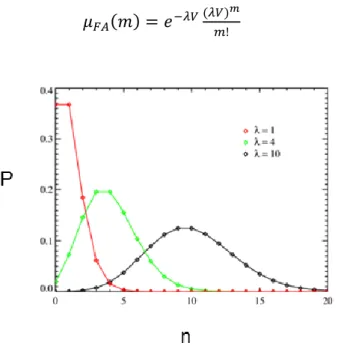
Let us now consider the limiting case +∞, that is we reduce the cell size until the continuous case. Then, the Binomial becomes a Poisson distribution with

( ) 𝑒 ( ) (3.3)

Therefore the pmf of the number of false alarms or clutter points in the volume , in terms of their spatial density λ, is given by

( ) 𝑒 ( ) (3.4)

Fig. 3.3 False alarms distribution in function of their spatial density

This serves as justification for the common use of the Poisson distribution for the number of false measurements in a certain volume under the two assumptions given above.

(52)

38

The spatial distribution of the false alarms is uniform, thus, neglecting the granularity due to the resolution cells, the probability density function (pdf) of the location of a false alarm is

( | 𝑒 ) (3.5) where V denotes now the volume of the subspace in which the measurement is known to lie. Depending on the situation considered, this can be the sensor’s surveillance region or a target’s validation region [35].

3.4 Single target tracking

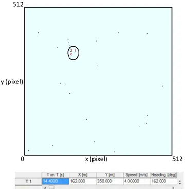
Initially, the case of application of KF and the Cheap PDAF in a scenario in the absence of false alarms is shown. The trajectory of the target estimated by the algorithms in three different instants of time is illustrated in Fig. 3.4a-c, respectively.

(53)

39

Fig. 3.5b Single target without clutter (acquisition time t2)

Fig. 3.6c Single target without clutter (acquisition time t3)

In each figure a table reporting the current state of various targets is given. In particular:

(54)

40

1. the first column represents the number of identified target;

2. the second column represents the Time on Target (T on T), which is how long the algorithm follows that particular target;

3. the third column represents the position X, in meters, of the identified target;

4. the fourth column represents the position Y, in meters, of the identified target;

5. the fifth column represents the magnitude of the velocity in meters / second, the identified target;

6. the sixth column represents the direction, in degrees, at which the target is moving, respect to the image center.

Of course, in case of absence of false alarms, the two algorithms are equivalent, since they both correctly follow the target.

Then we have considered a scenario where false alarms occurs. In the worst conditions, it has been assumed that, in each time instant k, three false alarms distributed randomly were present in the scene of observation, as well as the measure relative to the target. Therefore, for each time instant, four measures are present in the scene of analysis: three are false alarms and one will be the real one associated to the target of interest.

In the following, the trajectory of the target estimated by the two algorithms in three different instants of time is illustrated.

(55)

41

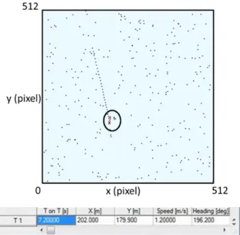
Fig. 3.7a Single target with clutter assuming 3 false alarms every time instant tracked

with NNSKF (acquisition time t1)

Fig. 3.8b Single target with clutter assuming 3 false alarms every time instant tracked

(56)

42

Fig. 3.9c Single target with clutter assuming 3 false alarms every time instant tracked

with NNSKF (acquisition time t3)

In figures 3.5a-c, the trajectory of the single target T1 is correctly estimated, in fact the value of the T on T in the tables is always growing.

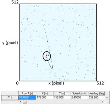
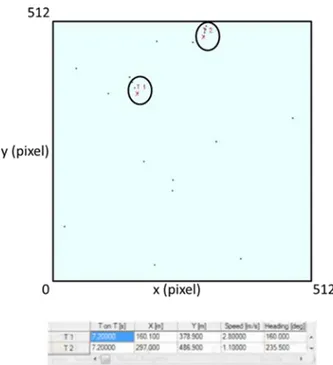
Subsequently, it was decided to further worsen the situation, working with 11 measures, 10 of which are false alarms and 1 measurement is really associated with the target.

Fig. 3.10a Single target with clutter assuming 10 false alarms every time instant

(57)

43

Fig. 3.11b Single target with clutter assuming 10 false alarms every time instant

tracked with NNSKF (acquisition time t2)

Fig. 3.12c Single target with clutter assuming 10 false alarms every time instant

(58)

44

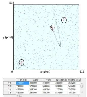
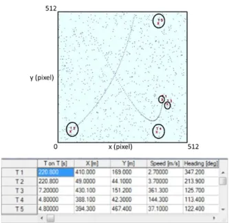
Figures 3.6a-c shows that the target T1 is followed by the tracking algorithm with some difficulties, in fact a consistence presence of false alarms can be noticed. Moreover, in Fig. 3.6b only two false alarms are present (one is named T1, as the target of interest, but it cannot be the target because it is completely outside the old trajectory), but, in this particular time instant, the trajectory is lost. Moreover, in figure 3.6c, in addition to the target of interest T1, also another target, T4, is detected near T1: this is due, essentially, to the problem concerning the association procedure; in particular, it is shown the case in which it wrongly attributes the origin of a measurement to the target of interest, since, among all the measurements present within that gate, one of these false alarms was also chosen as a measure originated from the target. The following Figures 3.7a-c will show the validation of the Cheap PDAF on the same simulated data

(59)

45

tracked with Cheap PDAF (acquisition time t2)

tracked with Cheap PDAF (acquisition time t3)

Also in this case, the target T1 is correctly tracked by the algorithm, regardless the presence of some false alarms. However, sometimes it is lost, in fact the

(60)

46

value of T on T related to this target is growing in Fig. 3.7a-b, but it is decreasing in Fig. 3.7c.

As in the NNSKF case, in the following figures we further complicate the problem, working with 11 measures, 10 of which are false alarms and 1 measurement is really associated with the target.

tracked with Cheap PDAF (acquisition time t1)

(61)

47

tracked with Cheap PDAF (acquisition time t3)

Figures 3.8a-c represents a situation similar to that shown on Fig. 3.7a-c, but in this case the presence of false alarms is very strong.

3.5 Multi target tracking

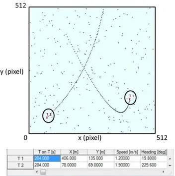
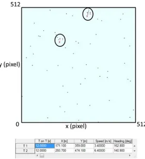
A scenario in presence of false alarms has been directly considered. As for the single target tracking case, in the worst conditions, it has been assumed that, in each time instant k, three false alarms distributed randomly were present in the scene of observation, as well as the measure relative to the target. Therefore, for each time instant, four measures are present in the scene of analysis: three are false alarms and one will be the real one associated to the target of interest.

In the following, the trajectory of the target estimated by the two algorithms in three different instants of time is illustrated.

(62)

48

Fig. 3.19a Two targets with clutter assuming 3 false alarms every time instant

tracked with NNSKF (acquisition time t1)

Fig. 3.20b Two targets with clutter assuming 3 false alarms every time instant