Volcano deformation in different tectonic settings using InSAR and modeling

Volcano deformation in different tectonic

settings using InSAR and modeling

Adriano Nobile

Università degli Studi Roma Tre

Dipartimento di scienze

XXV Ciclo - Scuola Dottorale in

Geologia dell’Ambiente e Geodinamica

Tutor: Dr. Valerio Acocella

Co-Tutor: Dr. Joel Ruch

Dedicata ad Amelie,

i

Index

2.4 - Mean velocity map 20

2.5 - Ground deformation time series 21

2.6 - Analytical models 26

2.6.1 - Earth and Source Models 26

2.6.2 - Confidence Intervals 33

3 - Data processing

3.1- Dallol proto-volcanic system

3.1.1 - Introduction 33

3.1.2 - The Afar triple junction 39

3.1.3 - Dyke-fault interaction during the 2004 Dallol intrusion at the

northern edge of the Erta Ale Ridge (Afar, Ethiopia) 51 3.1.4 - 2005-2010 surface deformation time series at Dallol 66 3.1.5 - Testing possible surface deformation relationships between

Dallol and the Erta Ale Ridge 73

3.1.6 - Discussion 77

3.1.7 - Conclusions 79

3.2 - 1993-2011 InSAR measurements at Aso caldera (Japan)

3.2.1 - Introduction 81

3.2.2 - Tectonic setting 81

3.2.3 - Data 88

ii 3.2.5 - Conclusion 103 4 - General Discussion 4.1 - Discussion 105 4.2 - Conclusions 109 5 - Bibliography 111 Appendix A.1 - Introduction A - 1

A.2 – Volcano Database (Chaussard and Amelung 2012) A - 2

A.3 – roi_loop.sh A - 24

A.4 – Mean velocity deformation map script A - 26 Acknowledgements

1

Abstact: Magma movements from reservoir toward the surface are responsible for volcanic unrest. Unrest can culminate with an eruption or the volcanic system can return to quiescence if magma fails to reach the surface. However, magma movements produce effects that can be observed and measured at the surface: Seismicity, ground deformation and gas emission; monitoring these geo-indicators at unresting volcanoes allow to evaluate the probability of occurrence of an eruption and which type of eruption is expected in order to define the hazard. It is also necessary to monitor these geo-indicators between unrest periods in order to define the background behavior of the volcano.

Space geodesy techniques allow to monitor ground deformation. In particular InSAR technique allow to measure mm-scale surface displacements over time spans of days to years and over wide areas. Inverting these data using analytical or numerical models allow to obtain information about the deformation source.

I studied ground deformation using InSAR technique and I evaluated the deformation sources parameters with analytical models at two magmatic systems located in extensional and compressional settings.

The first target area is Dallol, a proto-volcano located along the Afar rift axis; here I studied deformation associated to the October 2004 dyke intrusion that highlighted the presence of magma at shallow depth below the hydrothermal field, in an area without evidence of volcanism, and provided new information about the extension mechanisms along the rift segment. Furthermore, I produced ground deformation time series between 2005-2010 for an area that cover Dallol and the Erta Ale Ridge, another volcanic segment located along the Afar rift axis. This data suggest that Dallol subsided after the dyke intrusion whereas Alu Dalafilla and Erta Ale caldera uplifted. Data inversion for the subsidence at Dallol suggest the presence of a shallow deflating source.

The second target area is Aso Caldera that belongs to the Japanese South West volcanic arc. I studied ground deformation between 1993-2011 using different SAR sensors. I observed small displacement associated to eruptions. In particular I inverted InSAR data for a subsidence period between 1996-1998 caused by a deflation of a deep magmatic source just after the last phreato-magmatic eruption.

Finally I compared results on the magmatic sources at Dallol and Aso with those of volcanic systems located along divergent plate boundary and intra-arc volcanoes to verify if there are similarities between volcanoes that belong to the same tectonic setting.

2

1 - Introduction

Eruptions are generally preceded and accompanied by volcanic unrest, indicated by variations in the geophysical and geochemical state of the volcanic system. Such geoindicators commonly include changes in seismicity, ground deformation, nature and emission rate of volcanic gases, fumarole and/or ground temperature. This geoindicators can be observed and measured at the surface.

Volcanic unrest is related to magma movements from reservoir towards the surface (Fig.1.1 – e.g. Dvorak and Dzurisin, 1997). Magma intrude the host rocks forming conduits, sills, dykes and produce cracks that can depressurize the reservoir causing magma degassing. Fluids upward migration and heat flow changes can influence the behaviour of the shallow hydrothermal field even producing phreatic eruptions. However, not all volcanic unrest culminates in eruptions: in many cases the rising magma fails to breach the surface to erupt.

It is very important to monitor seismicity, ground deformation and gas emission and collecting information about eruptive histories of unresting volcanoes in order to evaluate the probability of occurrence of an eruption and also which type of eruption is expected, in order to define the hazard.

3

To define the volcanic unrest is essential to characterize the background level of these geoindicators; This requires to monitor volcanic areas also during quiescent periods and collecting information about the plumbing system.

In the last 40 years monitoring of active volcanoes increased its efficiency (e.g. Dzurisin, 2003; 2007) and in particular in the last 20 years the evolution of space geodesy techniques (GPS and InSAR) allowed scientist to better understand magmatic processes and to investigate volcanic unrest episodes studying ground deformation with high resolution data (e.g. Fournier et al., 2010, Chaussad and Amelung, 2012).

Fig. 1.2 Global map of volcanoes (black triangles) (Smithsonian Institution, Global volcanism report, available at http://www.volcano.si.edu) with areas of observed volcanic deformation shown as red triangles (Fournier et al., 2010).

Actually more than 1500 volcanoes are considerate active (Fig. 1.2) but just 800 are geodetically monitored (Fournier et al., 2010; Chaussard and Amelung, 2012). In many cases it is possible to know the state of a volcano in real time; however several magmatic systems are still poor studied.

Seismicity remains an important parameter used to forecast eruptions (e.g. Fig. 1.3); however geodetic and geochemical data are becoming progressively more and more important, so that a combination of the three types of data is required to understand unrest

4

episodes, to forecast any eruption and to study the volcano eruptive cycle, that is the combination of all the processes from deep magma generation through surface eruption, including such intermediate stages as partial melting, initial ascent, crustal assimilation, magma mixing, storage, degassing, partial crystallization, and final ascent to the surface (Dvorak and Dzurisin, 1997; Dzurisin, 2003; 2007; Fournier et al., 2010).

Fig. 1.3 A comparison of RSAM (real-time seismic amplitude measurement) culminating in eruption at three volcanoes. Mount St. Helens (May 1985 dome building), Mount Pinatubo (eruption of June 7, 1991), and Mount Redoubt (eruption of January 1990). (Endo et al., 1996).

There are several examples of how multidisciplinary volcano monitoring mitigated hazard and prevent causalities. The first and most famous is the reawakening of Mount St. Helens (Washington USA) in 1980, after 123 years of inactivity, that was correctly recognized from an unusual seismicity beneath the volcano on March 1980. A whole monitoring revealed patterns of earthquakes, ground deformation and volcanic gas emissions that preceded the first of six eruption in 18 may 1980 (Swanson et al., 1983; Brantley and Myers, 2000). USGS scientists saved thousands of lives evacuating the area before the eruption.

Another case is the Pinatubo volcano (Fig. 1.4), Philippines, that in 1991 produced one of the world's largest eruption of the 20th century (VEI 6 – Smithsonian Institution, Global volcanism report, available at http://www.volcano.si.edu). Between March-April 1991, a seismic swarm occurred on the north-western side of the volcano. On April 2, the volcano awoke after ~500 years of quiescence, with a phreatic eruptions occurring near

5

the summit. Volcanic activity increased throughout May. A rapid increase of sulphur dioxide emissions suggested that fresh magma rise up beneath the volcano. The first magmatic eruptions occurred on 3 June, and the first large explosion on 7 June generated an ash column 7 km high (Punongpayan et al., 1996).

Fig. 1.4 Pinatubo eruption (1991). http://vulcan.wr.usgs.gov

In many cases scientist forecasted the eruption but anyway this produced considerable damages because is not easy to predict the eruption type or all the phenomena that can combine with volcanic products (e.g. wind, rain, ice melting on the top of the volcano). For example the 2010 relatively small volcanic eruption of Eyjafjallajökull in Iceland caused enormous disruption to air travel across western and northern Europe between April and May (Petersen, 2010). About twenty countries closed their airspace. Unrest started at the end of 2009 with anomalous seismic activity that gradually increased in intensity until on 20 March 2010. Seismic data revealed that the eruption was preceded by several intrusions and highlighted the magma movements toward surface during the eruption (Tarasewicz et al., 2012a; Tarasewicz et al., 2012b).

Sometimes it is not easy to interpret the geoindicators and evaluate if a volcanic unrest will culminate in an eruption. Campi Flegrei Caldera (Italy) is experiencing an uplift

6

with a maximum rate of 3 cm/month measured with GPS and InSAR data (INGV – internal report). Seismic activity is not showing an anomalous behaviour compared to the background level (INGV – weekly bulletin). The last eruption in this area occurred in 1538 at Monte Nuovo (Rosi et al, 1983; De Vito et al., 1987). Deep structure of Campi Flegrei is well studied using different techniques, seismic tomography (e.g. Ferrucci et al., 1992; Zollo et al., 2003), gravimetric and magnetic data (Berrino et al., 1984; Barberi et al., 1991; Scandone et al., 1991;), inversion of geodetic data (Lanari et al., 2004; Battaglia et al., 2006; Gottsmann et al., 2006; Amoruso et al., 2008; D’Auria et al., 2012). Actually the Caldera is under close monitoring (e.g. Chiodini et al., 2012). Despite the large amount of information about this Caldera is not simple to understand if the uplift is related to a magmatic or an hydrothermal unrest.

What we actually know from literature about ground deformations before eruptions is that basaltic volcanoes generally inflate prior to eruptions (Wicks et al., 2002; Lu et al., 2010; Poland et al., 2012) instead the uplift at explosive, andesitic volcanoes is difficult to interpret (Fournier et al., 2010). There are many observations of inflation without eruptions, at Peulik, Akutan (Lu et al., 2007); Hualca-Hualca, Uturuncu, Lazufre (Pritchard and Simons, 2004); Laguna del Maule, Cordon Caulle, Cerro Hudson (Fournier et al., 2010). There are also examples of eruptions without precursory inflation at Shishaldin, Pavlov, Chiginagak, Veniaminof (Lu et al., 2007); Sabancaya, Ubinas, Lascar, Irrupuntuncu, Aracar, Ojos del Salado (Pritchard and Simons, 2004); Nevado del Chillan, Copahue, Llaima, Villarica, Chaiten, Reventador, Nevado del Tolima (Fournier et al., 2010); Galeras (Parks et al., 2011).

Ground deformations associated to aborted eruptions can be explained by magma overpressure remaining below a critical threshold (e.g., Pinel and Jaupart, 2004), by dikes stopping at various crustal levels without reaching the surface (Gudmundsson, 2006; Pallister et al., 2010; Nobile et al., 2012), or by changes in geothermal systems (Tait et al., 1989). Eruptions without precursory inflation suggests that volcanoes were in a critical state in which small perturbations lead to eruptions, or that they are lacking reservoirs at depths shallow enough to create detectable ground deformation (Fournier et al., 2010).

Actually, observations of pre-eruptive deformation at explosive andesitic volcanoes are limited to isolated cases. Increasing the number of monitored volcanoes will probably lead to a better understanding of the problem (Fournier et al., 2010; Chaussard and Amelung 2012).

7

Fig. 1.5 Satellite radar data spanning the 2005 Dabbahu main rifting event produced using data from ESA’s Envisat satellite. Left column (a, c, e) from descending track 49 using images acquired on 6 May and 28 October 2005, right column (b, d, f) from ascending track 29 images on 28 July 2005 and 26 October 2005. a, b, Wrapped interferograms; c, d, range change (unwrapped interferogram where available, range offsets elsewhere); e, f, azimuth offsets. LOS, satellite line of sight. (Wright et al., 2006).

Measuring ground deformation in volcanic areas also allow to relate magmatic processes to those tectonics. For example geodetic data for the rifting episode occurred between 2005-2009 in North Afar along the Dabbahu-Manda Hararo rift segment highlighted that extension occurs through repeated magma intrusions and dyke-induced faulting (Sigmundsson, 2006). This rifting episode consist of a sequence of 13 dyke intrusions accompanied by thousands earthquakes with magnitude ranging between 2-5; these intrusions were observed using InSAR (e.g Fig. 1.5), GPS and seismicity (Wrigth et al., 2006; Hamling et al., 2009; Grandin et al., 2010; Ebinger et al., 2010; Belachew et al., 2011). The intrusions involved an area 80 km long with 3 km3 of intruded magma (Ebinger et al., 2010; Nobile et al., 2012).

8

Another dyke intrusion occurred between August – July 2007 at Lake Natron (Tanzania) along the East African Rift System axis. In this case InSAR data and seismicity allowed to understand that a Ml = 5.9 earthquake produced the pressure change that

triggered the dyke intrusion (Calais et al., 2008; Biggs et al., 2009).

In this thesis, using InSAR technique (Goldstain et al., 1988; Massonet and Feigl, 1998; Madsen and Zebker 1999; Rosen et al., 2000) I studied surface displacements and using analytical models (Mogi, 1958; Okada, 1985; McTigue, 1987; Yang et al., 1988; Cervelli et al., 2001; Fialko 2001; Wright et al., 2003; Amoruso and Crescentini, 2009) I evaluated the deformation sources at two magmatic systems, located in different tectonic settings in order to understand nature and features of the magmatic systems, to study the volcanic cycle and to relate ground deformation to the regional tectonic setting.

To produce interferograms I used ROI_PAC software (Rosen et al., 2004), the Jet Propulsion Laboratory (JPL – NASA) release; I wrote a Linux shell script in order to improve this software and manage a great number of data, running it in loop (Appendix A.2). I also wrote a Matlab function to post-elaborate interferograms making simple corrections and creating mean deformation velocity maps (Appendix A.3). Furthermore I used -rate software (Biggs et al. 2007; Elliott et al., 2008; Wang et al. 2009; Wang et al., 2012) to produce ground deformation time series. At least I used a non linear inversion software (Cervelli et al., 2001) to invert ground deformation data.

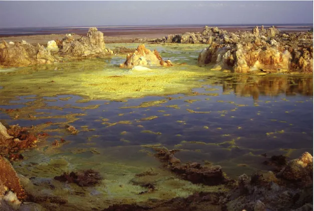
The first target area is Dallol magmatic system that is an hydrothermal field (Fig. 1.6) located along the northern Afar rift axis (Ethiopia), in a seafloor spreading area (Carniel et al., 2010; Nobile et al., 2012). Due to the remoteness of the area, few direct observations of Dallol have been made and volcanic products have not been found. InSAR data allowed to appreciate the surface deformation at Dallol, which would have been otherwise unnoticed because no instrumental monitoring was made. I studied ground deformation associated to a dyke intrusion occurred at Dallol between 22 October and 4 November 2004, that was not accompanied by an eruption but demonstrated the presence of magma at shallow depth, below the hydrothermal field. I also studied the surface displacement at Dallol for the period following the intrusion between 2005-2010. Results for the inversion of a subsidence period between 2008 - 2010 suggest the presence of a shallow deformation source. In order to contextualize surface displacements at Dallol with the regional tectonic setting I produced a deformation time series between November 2005 - February 2010 that cover also the area of the Erta Ale Ridge, a volcanic system located tens km south of

9

Dallol (Barberi and Varet, 1970). Results suggest a correlation between ground deformation in Dallol, Gada Ale, Alu Dalafilla and the Erta Ale Caldera.

Fig. 1. 6 Dallol hydrothermal field. Shot by Valerio Acocella (2003).

The second study case is Aso Caldera located in Southwest Japan on Kyushu Island (Sudo et al., 2001; Kaneko et al., 2007; Myabuchi et al., 2008; Abe et al., 2010; Unglert et al., 2011). Aso is one of the largest caldera belonging to the Japanese southwest volcanic arc. Several post-caldera cones are located in the central part of the caldera, among which Naka Dake, the only still active (Fig. 1.7), characterized by strombolian and phreatic activities (Kenda et al., 2008; Miyabuchi et al., 2008; Miyabuchi and Terada, 2009). Aso Caldera is in continuous unrest as highlighted by the frequent eruptions (seven in the last 20 years) the last in May – June 2011, the high geothermal activity, seismic swarms and ground deformation (Hase et al., 2005; Miyabuchi and Terada, 2009; Unglert et al., 2011; Terada et al., 2012). I produced interferograms that cover the period between 1993-2011 using four different SAR sensors (ERS_1, ERS_2, ENVISAT and ALOS). I inverted the signal obtained for a subsidence period between January 1996 - November 1998, just after the last phreato-magmatic eruption that occurred between May 1994 - November 1995, obtaining a deformation source at 6-7 km of depth. Ground deformations observed with InSAR data and inversion results are in

10

agreement with available GPS and seismic data (Sudo and Kong., 2001; Ohkura and Oikawa, 2008; Abe et al., 2010; Unglert et al., 2011).

Fig. 1. 7 Naka Dake crater filled by an acid lake. (www.aso-geopark.jp)

The choice of these two areas was based on (1) the availability of SAR data, (2) to not overlap with other work-groups, and (3) for their peculiar feature: Dallol is a proto-volcanic system, poorly studied, without evidence of proto-volcanic products, located along the Afar rift axis and with high ground displacements and seismicity. Aso Caldera is a well monitored, large volcanic complex, with frequent eruptions and with small ground deformation.

Furthermore I compared the obtained results about Dallol and Aso Caldera deformation sources with data available in literature about other volcanic systems that belongs to the same regional tectonic settings. I improved a pre-existing database of volcanic-arc magmatic source depth (Chaussard and Amelung, 2012) collecting information about magma reservoir in volcanic systems located along divergent plate boundary.

11

2 – Methods

2.1 Introduction

Measuring surface deformation in volcanic areas allows to obtain information about the nature and evolution of a magmatic system. Magma movements produce ground displacement and are frequently related to eruptions; so it is useful to use geodesy in order to evaluate the hazard in unresting volcano.

InSAR is the acronyms of Interferometric Synthetic Aperture Radar; this technique was developed during the ’80s but expanded in the ‘90s after the orbit of the European Space Agency Satellite ERS-1 in 1991. InSAR allow to measure mm-scale surface displacements over time spans of days to years (Massonnet and Rabaute, 1993; Zebker et al., 1994; Massonnet and Feigl, 1998; Burgmann et al., 2000; Rosen et al., 2000; Dzurisin, 2007).

Inverting the obtained deformation maps using analytical or numerical models may provide information about the deformation source (Mogi, 1958; Okada, 1985; McTigue, 1987; Yang et al., 1988; Cervelli et al., 2001; Fialko 2001; Amoruso and Crescentini, 2009).

In this chapter I will describe the InSAR processing technique and additional techniques to use interferograms in order to increase reliability of data and produce velocity maps and deformation time series as well as analytical inversion techniques.

2.2 InSAR processing

2.2.1 SAR technique

A satellite in polar orbit passes over the same area with the same orbital parameters every 30-50 days (depending on the altitude and orbit inclination; Fig. 2.2.1). The satellite is equipped with an antenna that sends an electromagnetic signal at a precise wavelength and receive the reflected signal by the surface. Typical wavelength are in X-band, C-band and L-band that corresponds respectively to ~3 cm, ~6 cm and ~24 cm.

Using particular algorithms that take advantage of physical phenomena like Doppler effect and chirp sonar, a synthetic aperture radar (SAR) image is created. A focused SAR image contains information about the SAR-to-surface range, the radar beam’s two way transit through the atmosphere, and its interaction with a myriad of small reflectors on the ground. When the signal scattered from a given resolution cell on the ground is received

12

back at the SAR, it contains a microwave fingerprint of the cell encoded as amplitude (i.e., intensity or brightness) and phase information, which is mathematically distinctive. This information can be recorded as a single complex number Aeiϕ, with A representing the amplitude of the echo and ϕ representing its phase. A fully focused SAR amplitude image is similar in many ways to an aerial photograph with a spatial resolution of ~10 m (e.g. Fig. 2.2). Instead the SAR phase image is totally random (e.g. Fig. 2.2), but it contain information about the ray-path and if this is used with other SAR images acquired in successive satellite pass, allows to detect any ground deformation occurred between two acquisitions or to create a Digital Elevation Model (DEM).

Fig. 2.1 Advanced Land Observing System (ALOS) orbit track. This was the Japanese satellite equipped with a SAR that worked in L-band. It acquired images between January 2004 – April 2011 with a 46 days of recurrence cycle.

2.2.2 Principles of InSAR

It is possible to map the Earth surface with SAR from an aircraft or satellite at meter-scale resolution, but to produce a DEM or to image centimeter-meter-scale surface displacements requires some additional cleverness and mathematical manipulation. First, it is necessary a pair of overlapping radar images taken from slightly different vantage points. Overlapping radar images can be obtained in two ways. First, an aircraft or satellite can be equipped with two spatially separated antennas. One of the antennas serves as both transmitter and receiver, while the other serves as a second receiver. The images produced by the antennas are similar but subtly different owing to the different viewing

13

geometries. NASA used this single-pass, dual antenna approach for its Shuttle Radar Topography Mission (SRTM), which mapped approximately 80% of Earth’s land surface between 60°N and 56°S during an 11-day flight in February 2000 (Farr and Kobrick, 2000;

Fig. 2.2 Two SAR images of the same target area (top and middle) acquired at different times and from slightly different vantage points, with perpendicular baseline 35 m. They are co-registered to produce an interferogram by differencing the phase values (bottom) . The resulting interferogram contains fringes produced by the differing viewing geometries (orbital fringes), topography (topographic fringes), any path delays present in the images, and surface displacements (deformation fringes). These images of Mount Peulik Volcano, Alaska, were acquired by ERS-1 on 4 Oct. 1995 (top) and ERS-2 on 9 Oct. 1997 (middle). Dzurisin (2007).

14

Williams, 2002). For SRTM, the SIR-C/X-SAR radar system was augmented by secondary C-band and X-band receive (slave) antennas mounted at the tip of a 60m boom that could be extended from Space Shuttle Endeavor’s cargo bay to form a single-pass interferometer (Bamler et al., 1996; Jordan et al., 1996; Farr and Kobrick, 2000). Another way to obtain overlapping radar images is to observe the same land area at least twice with the same radar by returning to nearly the same vantage point at different times.

(a) Co-registration of overlapping radar images: The first step in producing an

interferogram is to co-register the two radar images so that we can difference (subtract) the phase information from corresponding pixels. The separation of image-acquisition points, or the distance between the SAR trajectories at the times of the two image acquisitions, is called the baseline. For long baselines (>1 km), differences caused by topography and viewing geometry can be too severe for coherence to persist. In such cases, the images are said to be spatially decorrelated. If the spatial coherence is good, it is possible to use both the amplitude and phase information to co-register the images. The two sets of phase data are random but in a similar way, so they are helpful if they are spatially coherent. Otherwise, the amplitude data alone are generally sufficient. Think of the amplitude and phase data as two layers of a single image. These layers are perfectly co-registered for each image, but corresponding pixels in the two images are offset from one another owing to the different viewing geometries and topography. Conceptually, it is necessary to slide the two images over one another and distort them to achieve the best possible alignment of corresponding pixels. In practice this procedure is accomplished using the cross correlation to determine the offsets between corresponding pixels. In one coregistration algorithm, a Fast Fourier Transform (FFT) is first run on a down-sampled version of each single-look complex (SLC) image. The FFT of the first image is multiplied by the conjugate of the FFT of the second image to compute the correlation matrix in the frequency domain, and an inverse FFT is run on the product to return to the spatial domain. The location of the peak in the correlation matrix approximates the overall offset between the images. This result is refined by selecting corresponding, full-sampled portions from near the center of each image, using the approximate offset determined earlier, and repeating the procedure. Finally, the images are divided into sections called chips and the correlation procedure is repeated on corresponding chips to determine the offsets between each of them as a function of position in the image. By fitting a polynomial to the results (second-order is sufficient in most cases), co-registration at the subpixel level

15

can be achieved throughout the entire image. The second image is then re-sampled into the viewing geometry of the first so the pixels in both images correspond precisely.

(b) Creating the Interferogram: When two images have been successfully

coregistered, it is possible to produce an interferogram simply by differencing the phase values of corresponding pixels (Fig. 2.2). The phase value associated with each resolution cell on the ground is determined in large part by the properties of numerous elementary reflectors within the cell, which combine to produce a unique phase signature. If these properties do not change appreciably between the acquisition times of the first and second images, their random contributions vanish in the difference image (i.e., the interferogram) and a nonrandom, useful information is obtained.

An interferogram produced in this way includes contributions from the different viewing geometries of the two parent images, topography, path delays owing to different atmospheric conditions, noise, and any range changes caused by surface deformation during the interval spanned by the image acquisitions.

First it is needed to remove or account for the other sources of phase differences in the interferogram.

(c) Removing the effects of viewing geometry and topography: The difference in

viewing geometry between two images acquired from slightly different vantage points produces a regular pattern of phase differences between the images. If the target area were perfectly flat, these differences would manifest themselves in the interferogram as a series of nearly parallel bands called orbital fringes (Fig. 2.3). These can be computed and removed based on the known trajectory and imaging geometry of the SAR, along with the small additional effect of Earth’s curvature. The result is called a flattened interferogram.

Surface topography also contributes to the phase images, which is helpful if our goal is to produce a DEM but superfluous if the real interest is ground deformation. In the latter case, the effect of topography can be removed from a flattened interferogram by first constructing a synthetic interferogram based on known topography (i.e., on a DEM). A useful concept in this regard is the altitude of ambiguity ha which is the amount of surface

height difference that would produce exactly one topographic fringe:

𝑕

=

16

where H is the satellite altitude, λ is the wavelength of the SAR,  is the incidence angle, and b is the perpendicular component of the baseline with respect to the incidence angle

Fig. 2.3 Orbital fringes can be computed from the known trajectory and imaging geometry of the SAR and removed from the initial interferogram by subtraction (top) to produce a flattened interferogram. Similarly, topographic fringes can be removed by subtracting a synthetic interferogram (middle) based on the known topography (e.g. DEM) to produce a topography removed interferogram, which includes fringes produced by surface displacements (deformation fringes) and any path delays present in the images, plus noise. Spatial filtering suppresses the noise and accentuates the fringes (lower right). Dzurisin (2007).

17

. For example, ha 10 m means that, for a given image pair, each 10 m of surface height

difference would produce one topographic fringe in the interferogram, which would resemble a topographic map with a contour interval of 10 m. Given ha for a particular image pair, it is relatively straightforward to produce a synthetic interferogram that simulates topographic fringes. Subtracting the synthetic interferogram from the observed flattened interferogram, we are left with a topography removed interferogram that contains only the effects of noise, path delays, and (most importantly) surface deformation (Fig. 2.3).

Fig. 2.4 Displaying an interferogram over an amplitude image facilitates visual correlation of fringes with surface features (B). Images A and B are displayed in the SAR viewing geometry. Because the orbit and imaging characteristics of the SAR are known, the interferogram and amplitude image can be georeferenced (i.e., rectified to geographical coordinates) for consistency with standard map products (C) (Williams, 2002), and the rectified interferogram can be displayed over a shaded relief image produced from a digital elevation model (D). Each fringe corresponds a 0-2 phase variation i.e. to λ/2 range change (2.8 cm in this case). The concentric pattern indicates ~17cm of uplift centered on the southwest flank of Mount Peulik Volcano, Alaska, which must have occurred sometime during the interval spanned by the interferogram (October 1995-October 1997). Dzurisin (2007).

18

Any errors in the DEM used to produce the synthetic interferogram will remain in the topography removed interferogram, so for deformation studies it is important to choose image pairs with a large altitude of ambiguity (i.e., short baseline). An interferogram formed from such pairs will have low sensitivity to DEM errors but full sensitivity to surface displacements. Conversely, if the goal is to produce a DEM from the interferogram, a small ha value (long baseline) is desirable for better sensitivity to topography.

A topography removed interferogram can be spatially filtered to reduce the effect of short wavelength noise, and displayed over an amplitude image to facilitate visual correlation of deformation fringes with surface features (Fig. 2.4(A) and (B)). A final step to enhance the utility of the interferogram is to rectify (warp) the image to a geographical coordinate system, so that it can be displayed over a shaded relief image derived from the DEM or with other georeferenced map features (Fig. 2.4 (C) and (D)).

(d) Range-change resolution of InSAR: Using InSAR is possible to image topography with ~10 m resolution, and it is also possible to measure millimeter-scale surface displacements. If part of the target area moves toward or away from the satellite during the time between two image acquisitions, the round-trip distance would have changed; This means that the phase signals reflected from the same resolution cell in the two images (after corrections for viewing geometry and topography) would be varied of a quantity proportional to the displacement.

Phase signal can vary between 0 and 2. A phase difference of 2 correspond to a displacement of λ/2, where λ is the radar wavelength. However there is an ambiguity because to a displacement di corresponds a phase change Δϕi, but to a displacement dj =

di + λ/2 corresponds the same phase change Δϕi. The process to solve this ambiguity and

convert the phase variance in displacement in cm is called unwrapping. There are several algorithms that allow to unwrap phase variance as the Statistical-cost Network-flow algorithm (Chen and Zebker, 2002) or the brunch-cut algorithm (Goldstein et al., 1988).

So the range-change resolution depends on the radar wavelength (3.1 cm for the X-band, 5.6 cm for the C-band and 23.6 cm for the L-band) and on the precision in measuring the phase variance. By interpolation, we could in theory measure surface displacements corresponding to a small fraction of λ/2, perhaps as little as 1 mm. In practice, various sources of image noise, mostly phase delays caused by inhomogeneity in the troposphere and ionosphere, limit the range-change accuracy of interferometry to 1–10 mm under favorable conditions. A crucial assumption in the foregoing discussion is that nothing in the target area changed during the time between successive radar images other

19

than the surface height. This is not necessarily true over timescales of days to years, which are of interest for volcano monitoring. Over that period of time, vegetation might grow or die, rainfall might change the soil moisture, snow might accumulate or melt, or the surface might be affected by erosion or deposition. If such non-deformation changes are large with respect to the radar wavelength, our attempt to co-register the images and form a useful interferogram might fail. In this case, the images are said to lack coherence or be temporally decorrelated.

2.3 ROI_PAC

In order to produce interferograms I used the open source software Repeat Orbit Interferometry package (ROI_PAC Version 3.0.1), developed by the Jet Propulsion Laboratory (JPL) - NASA - Caltech (Rosen et al., 2004). This software is configurable to work with SAR images from different satellites. ROI_PAC community developed several tools that allow to convert Level-0 images from several satellites to raw radar data. I worked with SAR images by European Space Agency (ESA) spacebornes as ERS-1, ERS-2 and EnviSAT and by Japan’s Advanced Land Observing System (ALOS). ROI_PAC uses raw radar data, ancillary information from telemetry and navigation solutions, and digital elevation models (DEM; externally provided or interferometrically derived) to produce a variety of derived data products, including full resolution images, interferograms, phase images measured as principal value and continuously "unwrapped" DEMs, and error estimates. It uses the branch cut algorithm to unwrap phase differences (Goldstein et al., 1988) but it support also other algorithms. Each of the products is available in its natural radar coordinate system and is georeferenced to a DEM. The software computes the interferometric baseline from the navigation solutions provided, and then refines the estimate to the millimeter level of precision using the DEM provided and the optional deformation model for reference. To remove the topographic signature from an interferogram, ROI_PAC simulates an interferogram from the orbit data and the DEM, and subtracts the phase from the measured interferogram, leaving just the deformation phase. ROI_PAC implements its fundamental algorithms in C and Fortran 90, and drives each executable module with a Perl control script.

ROI_PAC source code is available to the international community for research purposes from the NASA Open Channel software distribution system (http://www.openchannelfoundation.org).

20

2.4 Mean velocity map

Using InSAR technique is possible to produce maps of ground displacement over wide areas but it is still difficult to measure slow, small and long wavelength deformation signals due to spatial and temporal decorrelation, orbital errors and atmospheric errors (e.g. Biggs et al., 2007; Eliot et al., 2008). In order to reduce the impact of these factors on mine measurements and increase the reliability of data, I have created an original algorithm consisting of four stages: (a) relate observed ground displacement to a stable reference point; (b) correct for signal/topography correlation; (c) create a velocity map; (d) stack rate maps and evaluate a mean deformation velocity map.

(a) Reference point: The signal amplitude observed in one pixel is related to the reference point chosen to unwrap the interferogram. This reference point can change for each interferograms and sometimes it is not a real zero deformation point. It is very useful, in order to elaborate contemporaneously several interferograms, to refer ground displacement to the same reference point that can be considered stable.

The reference point must be coherent in each interferogram. A single pixel can be affected by random noise, so it is better to choose an area; in particular I consider 1 km2 area. I calculate the average signal in the area and I subtract this value to each interferogram pixel. The chosen area becomes a zero deformed area and the signal at each pixels is related to this area.

(b) Correlation signal/topography: During InSAR processing a Digital Elevation Model (DEM) is introduced in the processing to remove the topographic component from the interferograms. When the DEM is not precise enough, residual topographic fringe patterns appear and can be misinterpreted or confused with the sought-after displacement fields (Bombrun et al., 2009). The residual topography signal Δϕ_topoi _{for the i-th}

interferogram can be expressed by (Zebker et al., 1994; 1997; Bombrun et al., 2009):

Δ𝜙

=

𝜆 𝐵_⊥𝑖

𝐻 sin 𝜃

Δ𝑧

where  is the radar wavelength,

𝐵

Correlation between the signal and topography can be assumed linear. By calculating a linear regression between the interferogram signal and the topography for

21

each pixel, and subtracting this synthetic signal to the interferogram it is possible to reduce the error due to this correlation.

(c) Velocity map: each interferogram, which measures the total deformation between the dates of the master and slave acquisitions, can be converted into an average deformation rate by dividing by the time span of the interferogram.

(d) Stacking: The simplest, stacking, works on the principle that the signal in the interferograms has a systematic pattern, while the atmospheric noise is random. Addition of N interferograms with equal duration has a signal N times larger than a single interferogram, but the noise is only 𝑁 times larger. The signal-to-noise ratio is improved by a factor of 𝑁 (Peltzer et al. 2001; Wright et al. 2001; 2004b; Fialko, 2006).

Dividing the stacked map by N is obtained a mean velocity map. Furthermore it is possible to save the information about the deformation rate also in pixels not coherent in each stacked interferogram. However to not introduce large errors I impose that pixels in the final velocity maps must be coherent in at least the 75% of the number of stacked interferograms and the value of this pixels in the stacked map is divided by the number of interferograms in which it is present in order to evaluate the mean deformation rate.

2.5 Ground deformation time series

In order to measure surface displacement rate and time evolution, I used -rate software (Biggs et al., 2007; Elliot et al., 2008; Wang et al., 2009; 2012). This software was written in order to estimate the interseismic deformation along the Denali Fault, Alaska, where the deformation rate is small, coherence is very variable and high atmospheric noise affects interferograms (Biggs et al., 2007). It is an iterative algorithm with three steps; orbital error correction, construction of a rate map, and estimation of the fault slip rate (Fig. 2.5). In this work I used only the first two steps in order to study ground deformation time series. The first step estimates and removes the orbital error on each acquisition. The second step estimates the best-fitting deformation rate at each pixel based on whichever interferograms are coherent and produces a rate map and an associated error map. The last step is to invert the rate map to find the best fitting displacement rate using assumptions about the geometry of the area.

(a) Network orbital correction: Most previous studies estimate the orbital contribution on interferograms individually. However, each acquisition is used to construct several interferograms and so it is possible to estimate the orbital contribution to a single

22

acquisition using constraints from many interferograms. Therefore, this software uses a network approach to empirically estimate the orbital error on each acquisition rather than each interferogram.

Fig. 2. 5 Flow chart showing the algorithm for analysing interseismic strain accumulation using distributed scatterer interferograms in areas where coherence is variable. Biggs et al., 2007.

Orbital contributions to interferograms behave in a conservative manner and can be thought of as the difference between the orbital contributions to each acquisition. Initially is assumed that the interferogram is dominated by the orbital contribution and any other contribution is considered a source of noise. Assuming a planar orbital error, for a pixel, p, at location [xp, yp], the phase in the interferogram, φlm can then be written as a linear

function of two parameters, u and v, for each of the acquisitions, m and n, and a reference frame shift for the interferogram, wmn

φ

= u

x

− u

x

+ v

y

− v

y

+ w

Similar equations can be written for each coherent pixel in each interferogram.

This approach separates the long wavelength component (due to orbital errors and long wavelength ionospheric and tropospheric delays), which behaves as a linear combination of the long wavelength components on the acquisitions, from the long wavelength tectonic signal, which is simply related to the duration of the interferogram.

23

Short duration interferograms, which are often ignored because they have only a small component of deformation, provide valuable additional constraints to improve the estimates of the orbital component.

The value wmn is a reference frame shift which takes into account the different

unwrapping reference point locations used when unwrapping each interferogram.

Problems of this kind are intrinsically underdetermined since there will always be at least one fewer interferogram than the number of acquisitions. For a system of N interferograms with P pixels constructed using A acquisitions, there are 2A + N unknowns and NP observations. However, not all these observations act as independent constraints, the rows of the design matrix are linearly related giving a rank of 2(A − 1) + N. A truncated singular value decomposition is used to find the minimum norm solution using a threshold of 2 × 10−9 for truncating the singular values. This approach distributes the remaining orbital error, which cannot be solved for, across the existing orbital corrections, leaving an additional planar tilt and offset which must be corrected for at a later stage in the algorithm. For 90 m resolution, each interferogram contains roughly one million pixels making a total of 4.4 × 107 observations. However, since orbital errors have long wavelength features, this stage can be carried out at a much lower resolution, for example a pixel size of 6.4 km reduces the number of observations to a more manageable 7500. The variance– covariance matrix for these observations would contain 55 million elements. Although the matrix would be sparse, it is assumed that the observations are uncorrelated and equally noisy and perform the inversion without a variance–covariance matrix. Once the orbital parameters have been estimated, they can be used to construct a full resolution version of the orbital contribution for each interferogram and then removed.

A comparison between the estimation of orbital errors using the network approach versus the simple planar approximation highlights a reduction of 5–10 per cent for the Residual Mean Square (RMS) misfit between input parameters and correction parameters. The accuracy of the ramp parameters for an individual interferogram depends on the coherent area available, so for interferograms with poor coherence, the errors on the estimated ramp parameters are large. Using the network approach is improved the estimates for these interferograms, by using information from interferograms for which the orbital parameters are best constrained. Hence an overall improvement in the orbital correction is produced despite is reduced the number of free parameters.

(b) Rate map formation: It is necessary to combine measurements from pixels which are coherent in some but not all the interferograms. To do this a least-squares

24

matrix inversion on a pixel-by-pixel basis is used to find the best fitting rate, rlos, from the

available interferograms at each pixel. 2𝜋



𝑻 𝑟

= 𝑷

where T is a vector containing the time-spans, [t12, t23, t34 . . . tmn]T , and P is a vector

containing the phase, [φ12, φ23, φ34 . . . φmn]T for each interferogram which is coherent at

that pixel.

The inversion is weighted using a variance–covariance matrix, P, to take into

account the atmospheric and orbital noise at each interferogram and the correlation between interferograms. The element σlm−nq of the variance–covariance matrix, P

corresponding to the interaction between interferograms lm and nq depends on the atmospheric error estimate for each interferogram σlm and σnq, the orbital error estimate on

each pixel, σp, and the correlation between interferograms.



= (





+



) 𝑐

If the interferograms, lm and nq, have a common master or a common slave (l = n or

m = q), clm−nq = 0.5; if the master of one interferogram is the slave of the other (l = q or m =

n), clm−nq =−0.5 and at l = n and m = q, clm−nq = 1. For the sake of simplicity, the

atmospheric error, σlm, on each interferogram is assumed to be constant.

Since a common reference pixel is used for all the interferograms, errors in the orbital adjustment increase with distance from this point. The orbital error parameter for each pixel, σp, is based on its distance from the reference pixel.

Since the inversion is carried out on a pixel by pixel basis, it is not necessary to include the spatial correlation between pixels. The rate and associated error at each pixel is given by,

𝒓

=

𝑻

_Σ

𝑻

𝑻

Σ

𝑷

Σ

= 𝑻

Σ

𝑻

25

The reliability of the values at each pixel depends on the number and distribution of interferograms which are coherent at that pixel; Therefore, using the values from the error map is possible to determine the intensity of the pixels such that bright pixels have low a

priori errors.

(c) Slip rate estimate: For an assumed fault geometry and locking depth, the rate of ground deformation expected for a nominal slip rate (1 mmyr−1) is modeled. Using a simple deep fault model is expected that the ground deformation scale linearly with slip rate so a direct comparison of the corresponding pixel values in the rate map and the forward model should result in a straight line. The noise free test shows perfect correlation between the forward model and rate map, with the slope of the line reflecting the slip rate. For the test including noise, the points no longer fit on a perfect straight line, but the correlation is clear.

Similarly, the forward model can be used as a Green’s function for a linear least-squares inversion to find the slip rate, s,

rp = s fp + gxp + hyp + q (2.8)

where rp are pixel values from the rate map and fp are the corresponding pixel values

from the forward model. The additional parameters g, h and q are included to allow for the planar tilt and offset between the forward model and rate map which resulted from in using the minimum norm solution to the network orbital correction. The inversion is weighted using a variance–covariance matrix, P which takes into account the error estimates on

each pixel and the spatial correlation between pixels. The elements, σjk, of the variance–

covariance matrix, P , are constructed using σjk = σjσkcjk , where σj are the error estimates

on each pixel producing during formation of the rate map and cjk is the spatial correlation

between the pair of pixels. The correlation coefficients, cjk is estimated using the

exponential form.

Since variance–covariance matrices are used to weight the inversions, an a priori estimate of the error on the slip rate is produced at each stage of the algorithm. This significantly underestimates the scatter in results, probably because the spatial correlation between pixels is underestimated, so it is preferable to use a Monte Carlo method for a more realistic error estimate.

26

2.6 Analytical models

Space geodesy has provided numerous, high-quality surface deformation data sets. Large continuous GPS network and Interferometric synthetic aperture radar (InSAR) provide deformation data.

These geodetic data can provide important constraints on fault geometry, slip distribution and magma movements in volcanic areas.

For this reason, I used and nearly automatic methods for rigorously inverting surface deformation fields for source type and geometry provided by Cervelli et al., 2001.

2.6.1 Earth and Source Models

Estimating source geometry from geodetic data requie a forward model of how the crust responds to various kinds of deformation sources. The most commonly used crustal model is the homogeneous, isotropic, linear, elastic halfspace, which is adopted here. In spite of its limitations, the elastic half-space model is widely used primarily because of the simplicity of the expressions for the surface deformation caused by uniform, rectangular dislocations (e.g. Okada,1985) and point sources (Mogi, 1958). Moreover, until recently, most geodetic data were not of sufficiently high quality to justify more complex crustal models.

(a) Inversion as Optimization: The relationship between the deformation field and the source geometry can be expressed by the following observation equation:

𝒅 = 𝐺 𝒎 + 𝜀 (2.9)

where d is the deformation data vector, m is the source geometry vector (e.g., for a dislocation length, width, depth, dip, strike, location, slip), and G is the function that relates the two. The 𝜖 term is a vector of observation errors.

For the source geometry estimation problem the data are related nonlinearly to the source parameters. For this reason, source estimation reduces to nonlinear optimization.

The optimal source model, 𝒎 , will minimize the misfit between observation and prediction. Therefore it is systematically searched the finite dimensional parameter space for 𝒎 , using G to predict the deformation field for a given m.

27

In order to quantify the misfit is used the weighted residual sum of squares, which can be normalized by the number of individual data, n, minus the number of estimated model parameters, p. This forms the "residual mean square error" (RMS), expressed as:

𝑅𝑀𝑆 =

𝑛 −𝑝 (2.10)

Where r = d - G(m) and  is the presumably known data covariance. Several statistical tests exist for evaluating the significance of the RMS (e.g.,t he 2 _{and F tests),}

but it should be emphasized that the validity of these tests, as well as the meaningfulness of the n-p normalization, depends on Gaussian noise and a linear relationship between model and data. Statistical tests on the RMS should therefore be regarded skeptically. The geodetic signal contains unmodeled deformation components such as those arising from elastic heterogeneity or anisotropy. This unmodeled signal contributes to the misfit, so the best fitting model for a particular data set may yield an RMS that is quite high. The "optimality" of our estimated source model is thus always conditional on the assumptions intrinsic to the forward model.

(b) Solving the Optimization Problem: Derivative-based algorithms, Levenberg-Marquardt or the method of conjugate gradients, offer the most straightforward and efficient approach to solving this optimization problem (Gill et al., 1981). However, because these algorithms depend on the gradient and higher-order derivatives to guide them through misfit space, they can get trapped in the first local minimum that they encounter and never find or even approach the global minimum. Consequently, these algorithms work well only when the initial guess is near the global minimum. A priori information can often provide a good initial guess.

Clearly, whether a derivative-based method (or any method that always moves "downhill") reaches the global minimum depends on where it starts. Moreover, it is observed that particularly in cases with low signalto-noise ratios (SNR), the misfit space often contains numerous local minima and lacks a deep, well-defined global minimum. Therefore it is only possible to endorse derivative-based methods as a solution to the geodetic inversion problem in cases characterized by both a high SNR and good geologic insight into the probable type and location of the deformation source. Even in these cases, it is essential to show that the optimization converges to the same minimum from many different starting values.

28

Another way to solve the optimization problem involves discretizing the misfit space and then searching exhaustively through the resulting grid. Exhaustive searches prove viable, however, only when the number of estimated parameters stays small. The number of possible combinations equals QP, where Q is the number of divisions in the grid and p is the number of parameters. Adopting a coarse grid does little to help the problem both because of the exponential growth and because an overly coarse grid might miss the part of the misfit space containing the global minimum. Random searches prove more efficient than exhaustive searches, but the increase in efficiency is not sufficient to overcome the exponential nature of the problem. For these reasons, neither exhaustive nor random searching seems useful for anything but the most modest source geometries and the simplest Earth models.

In spite of their inefficiency, exhaustive and random searches do not suffer from the local minimum problem. Beginning in the 1940s, mathematicians sought algorithms that combined the effciency of a derivative-based method with the robustness of a random search. The result was the Monte Carlo class of algorithms. The common feature that all algorithms of this class share is an element of randomness that permits an occasional uphill move, that is, the algorithms will not always move from a candidate model with higher misfit to a model with lower misfit. This feature permits Monte Carlo algorithms to escape local minima. Monte Carlo algorithms differ from "conventional" random search methods in that the former retain a directivity that engenders a high level of efficiency. The two Monte Carlo algorithms explored in this paper are simulated annealing (Metropolis et al., 1953) and the random cost algorithm of Berg (1993).

(c) Simulated annealing: In simulated annealing, the likelihood of choosing a higher misfit model over a lower one depends not only on the misfit difference between the two but also on the state of the annealing process at the time of the choice. The algorithm quantifies this state dependance in terms of a temperature. At high temperatures all source models have roughly equal chance of getting picked, while at low temperatures the algorithm favors low misfit models.

The specific annealing algorithm adopted here follows from the work of Metropolis et al. (1953) and Cruetz (1984). Called the "heat bath" algorithm it proceeds as follows. The initialization procedure consists of two steps: (1) set bounds on the values for all the model parameters (these bounds can come from geologic constrains or physical limitations) and (2) randomly pick an initial starting model. Cycle through the individual model parameters, m1 throughr mp. At each mi, compile a list of candidate models by varying mi while holding

29

parameters mji fixed at their current values. Next, calculate the misfit associated with each

model, and form a probability distribution according to

𝑝

~𝑒

where T refers to the current temperature and RMSk refers to the RMS of the model

corresponding to the k-th permissibile value of the i-th parameter. To update the value for the i-th model parameter, randomly sample from the distribution. Continue updating until all the parameters have been cycled through, then lower the temperature according to a "cooling schedule" and repeat until some termination criterion obtains. Usually, that criterion is some preset number of model updates or some time period. Alternatively, a "freezing" criterion can be used where the algorithm stops if the current model has remained unchanged for some specified number of iterations.

At high temperatures the annealing algorithm essentially functions as a random search. As the temperature cools, low misfits are preferred, but the random sampling ensures that they are not required. Occasional uphill moves occur; local minima are visited and exited. In the final stages of annealing, when the temperature is very low, the probabilities associated with low misfits become very high, making uphill moves extremely unlikely.

The most significant complication to the simulated annealing algorithm is the cooling schedule i. e. how the temperature changes as the annealing progresses. This plays a crucial role in the success or failure of the optimization. Rothmann (1985) defined a critical temperature at which the bulk of the annealing should, for maximum effciency, occur. In brief, at the critical temperature the system remains cool enough to favor low misfits but still high enought o escape local minima. Basu and Frazer (1990) developed a method to quickly find the critical temperature that greatly improved on Rothmann's trial and error approach. This method runs the annealing algorithm at a number of different fixed temperatures and defines the critical temperature as the temperature at which the algorithm retains a high degree of directivity yet can still easily escape local minima. At temperatures much higher than the critical temperature, the algorithm behaves very much like a random search, while at temperatures much lower than the criticalt emperature it behaves like (an inefficient implementation of) a derivative-based algorithm.

30

It has been found that for the geodetic inversion problem it is generally not necessary to calculate the critical temperature using the algorithm described by Basu and Frazer (1990). Instead using extensive trials, it has been derived a fast method of forming a cooling schedule that works well for the geodetic inversion problem: calculate the average RMS for 100 randomly selected models (Cervelli et al., 2001). The approximate critical temperature Tc can be found from

𝑙𝑜𝑔10𝑇𝑐 = 𝑙𝑜𝑔10 𝑀𝑆𝐸 − 2.5 (2.12)

The first term on the right side of (2.12) provides a natural scale for the misfit function, while the second term is derived empirically. Once a good approximation of the critical temperature has been found, a cooling schedule can be easily generated. Like Basu and Frazer (1990), is recommended that the bulk of the annealing time be spent at or near the Tc. Specifically, the cooling schedule should begin 1 order of magnitude higher

than Tc and end 1 order of magnitude lower. The number of iterations spent at a particular

temperature should decay rapidly with distance from Tc. It has been found that a Gaussian

distribution centered at Tc works well (Cervelli et al., 2001).

(d) Random cost: Random cost is an alternative Monte Carlo approach for nonlinear optimization problems with many local minima in a broad misfit space (Berg, 1993). It uses a simple stochastic process to enforce a random walk in misfit space, which enables it to overcome local increases in misfit to find the global minimum. It preferentially samples minima (or maxima) while thoroughly sampling the misfit space. Several tests indicate that it is significantly less efficient than simulated annealing, but it is much easier to implement because it does not require a specific cooling schedule (Cervelli et al., 2001).

The random cost approach begins by generating a set of trial models that span a region about an arbitrary a priori model. The method for generating the trial model set is not unique. Following Berg (1993) a geometric grid in parameter space is defined centered on the a priori model. A geometric grid provides a convenient means to simultaneously sample the parameter space both broadly away from the a priori model (i.e., thorough sampling) and densely near the a priori model (i.e., high accuracy).

In the discussion that follows, the "cost" function is the RMS misfit. The misfit difference, ∆, is determined for each trial model, such that ∆ is the difference between the misfit of the trial model and the misfit of the a priori model. ∆ is negative for trial models with an RMS smaller than the a priori model and positive for trial models with higher RMS.

31

For simplicity, complications that arise when the trial model RMS equals the misfit of the a priori model are ignored (see Berg (1993) for discussion). Let f- equal the average of all the negative ∆ (i.e., better trial models) and f+ equalt he average of all the positive ∆ (i.e., worse trial models). If the a priori model is not at a misfit extremum, the random cost method chooses a new a priori model from the existing trial models based on a probability function determined from f- and f+. Let two probabilities p- and p+ (p- + p+ = 1) be defined by

𝑝−𝑓−= 𝑝+𝑓+ (2.13) which yields

𝑝−₌ 𝑓+

𝑓+_+𝑓− (2.14)

Let r be a random number chosen from a uniform distribution between 0 and 1. If r ≤ p-, a new a priori model is randomly selected from the set of trial models with negative ∆; otherwise, it is selected from the set of trial models with positive ∆. A new set of trial models is generated about the new a priori model, and the process is repeated until a local minimum (or maximum) is encountered, that is, until no better (or worse) trial models are found. This model is recorded and then the process can be restarted at another randomly chosen a priori model.

When the a priori model is near a misfit minimum, negative misfit differences will, on average, have smaller magnitude than the positive cost difference (f- ≤ f+). From (2.14) this implies that p- will be greater than p+, so there is a greater probability that the next a priori model will be chosen from the set with negative cost differences and therefore be closer to the cost minimum. As the a priori models get closer to the misfit minimum, the probability increases that an even better a priori model will be chosen for the next iteration. Thus the random cost method preferentially samples the local minima. However, there always remains a finite probability that a poorer fitting a priori model will be chosen, enabling the random cost method to overcome local increases in the misfit function in order to locate the global minimum.

From the symmetry of (2.13) and (2.14), it should be noted that maximum misfits will also be preferentially sampled, that is, the algorithm preferentially visits extrema, not just minima. Since we are seldom interested in the model that fits the data worst, they are simply discarded those models corresponding to maxima in misfit space.