Nonlinear static procedures for analysis and retrofitting of existing buildings with dissipative braces

(1)

SCIENZE DELL’INGEGNERIA CIVILE

______________________________________________________

SCUOLA DOTTORALE / DOTTORATO DI RICERCA IN

XXVI CICLO

_______________________

CICLO DEL CORSO DI DOTTORATO

NONLINEAR STATIC PROCEDURES FOR ANALYSIS

AND RETROFITTING OF EXISTING BUILDINGS WITH

DISSIPATIVE BRACES

__________________________________________________

Titolo della tesi

XU LIU __________________

Nome e Cognome del dottorando

firma

PROF. CAMILLO NUTI __________________

Docente Guida/Tutor: Prof.

firma

PROF.ALDO FIORI __________________

(2)

Collana delle tesi di Dottorato di Ricerca In Scienze dell’Ingegneria Civile

Università degli Studi Roma Tre Tesi n° 45

(3)

(4)

Nonlinear Static Procedures (NSPs), often called pushover analyses, are deemed to be very practical tools to assess the nonlinear seismic performance of structures. The use of NSPs for the seismic assessment of plan regular buildings and bridges is widespread nowadays. The use of NSPs in the case of real existing structures, which are almost always irregular, has so far been studied by a limited number of authors. This fact limits the application of NSPs to assess current existing structures. In order to improve the use of NSPs in practical, the applicability of NSPs for analysis and retrofitting of existing buildings with dissipative braces is evaluated in this thesis. In this work, a more efficient incremental modal pushover analysis (IMPA) to obtain capacity curve of the structure to evaluate the seismic demand is proposed: the procedure allows defining the capacity curve based on the execution of a series of MPAs. The case studies chosen are a benchmark structure as the regular structure and a real existing reinforced concrete building, which shows a strong irregularity in plan and vertical.Comparative evaluation of the different commonly used NSPs, which are Capacity Spectrum Method (CSM) adopted in ATC-40, Displacement Coefficient Method integrated into FEMA356, and N2 method presented in Eurocode 8 and modal pushover analysis (MPA), to describe their relative accurancy and limitations. A displacement based design procedure of dissipative devices for seismic upgrading structures is applied to the exising builidng. The accuracy of the IMPA is evaluated by comparison with IDA curve for the regular and irregular structure. Force-based and displacement design procedure of passive energy dissipation devices are applied to retrofit a school building located in shanghai, the comparisons of the two design methods and the seismic behavior of the retrofitting structure with different passive energy dissipation devices are discussed.

(5)

Figure 2.1Conceptual diagram for transformation of MDOF to SDOF system ... 8 Figure 2.2(a) Capacity curve for MDOF structure, (b) bilinear idealization for the equivalent SDOF system. ... 9 Figure 2.3 Conceptual explanation of uncoupled modal response history analysis of inelastic MDF systems ... 17 Figure 2.4Properties of the nth-“mode” inelastic SDF system from the pushover... 19 Figure 3.1 Evaluation of the performance points (P.P.) for each capacity curve that belongs from the pushover analysis with the selected load distributions: proportional to Mode1..Mode n. ... 36 Figure 3.2 Construction multimodal capacity curve (MCC) from the IMPA procedure. By applying SRSS rule with the P.P. obtained with each load distribution (Mode1..Mode n) and for each intensity level (the response spectrum is scaled from lower to higher intensity levels) the MCC) can be obtained. ... 37 Figure 4.1 retrofitting existing building with base isolation ... 39 Figure 4.2 retrofitting existing building with dissipative braces ... 39 Figure 4.3 The mechanism of the base isolation and dissipative braces ... 41 Figure 4.4 Schematic mechanism of the BRB ... 42 Figure 4.5 Examples of BRB bracing configurations, a) Diagonal bracing, b) Chevron bracing, c) V bracing, d) X bracing (Tremblay et.at,2004) ... 43 Figure 4.6 Connection to steel structure ... 43

(10)

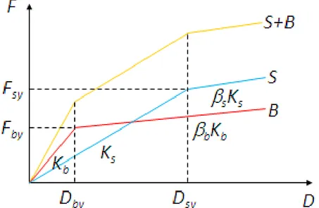
Figure 4.7 Connection to R.C. structure ... 44 Figure 4.8 Scheme of the braced structure (S+B) as sum of the existing structure (S) and the bracing system (B) ... 47 Figure 4.9 Interaction between the structure (S) and the bracing system (B) expressed in terms of horizontal components of the force-displacement relationship ... 47 Figure 4.10 Deformed shape of a generic single part of the braced frame ... 48 Figure 4.11 Evaluation of the equivalent bilinear capacity curve ... 54 Figure 4.12 Evaluation of the equivalent viscous damping needed to achieve the target performance point ... 56 Figure 4.13 Dissipative device “j” assembled in series with an extension element (e.g. a steel profile): equivalent model of springs in series (K’d,j; K’p,j) and equivalent single spring model (K’b,j) ... 57

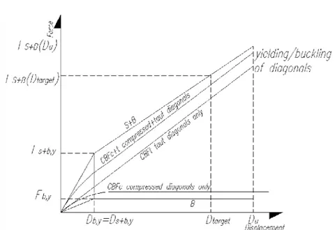
Figure 4.14 Force-Deformation of the existing structure (CBF) and of the retrofitted structure (CBF+dissipative braces). Dtarget is the target of the retrofitting design: diagonals must remain elastic and Dtarget<Du.

... 64 Figure 4.15 existing structure (CBF) under seismic action ... 65 Figure 4.16 Retrofitted structure (CBF+dissipative braces) before and during seismic action. The diagonals are still elastic and the dissipative braces are yielded Dtop after retrotting is limited in order to

obtain the retrofitting of the structure: Dtop=Dtarget>Du ... 66

Figure 5.1 Nine-storey building (adapted from Ohtori etc. (2000)). . 68 Figure 5.2 Response spectrum of 2/50 set of records ... 69 Figure 5.3 Response spectrum of 10/50 set of records ... 69

(11)

Figure 5.4 Response spectrum of 50/50 set of records ... 70

Figure 5.5 2D finite element model in SAP2000 ... 71

Figure 5.6 Plan layout of the existing building ... 72

Figure 5.7 Elevation layout of the existing building ... 72

Figure 5.8 Section A-A ... 73

Figure 5.9 Graphic documentation type for the project ... 74

Figure 5.10 Response spectra of the code-compliant set of Time Histories (TH): TH1..TH7 are the selected ground motion records, NTC’08 is the response spectra according to Italian technical code for a returning period of TR=949 years, Sa is the average response spectra from the set and Sa+σis the range of variation according to standard deviation ... 78

Figure 5.11 Code- compliant and earthquake acceleration horizontal response spectra ... 79

Figure 5.12 Natural accelerogram associated with SLV Tr = 949 years ... 79

Figure 5.13 Transverse sections of the building. ... 80

Figure 5.14 Longitudinal sections of the building ... 80

Figure 5.15 oblique views ... 81

Figure 5.16 simulation of shell wall ... 82

Figure 5.17 oblique view ... 82

Figure 6.1 Modal mass participation for the first three modes ... 84

Figure 6.2 Modal shapes for the first three modes ... 85

Figure 6.3 P.P. is determined via CSM from original and reduced demand spectrum for the first mode. ... 86 Figure 6.4 P.P. in terms of spectral acceleration and spectral

(12)

displacement can be converted to P.P. in terms of the roof displacement (Ur) and base shear Vbn corresponding to Ur from the

pushover capacity curve through Eq.(6.2) ... 86

Figure 6.5 P.P. is determined via N2 ... 87

Figure 6.6 Peak response of 50/50 set of records ... 88

Figure 6.9 Normalized lateral load distributions of 10/50 set of records ... 91

Figure 6.10 Peak response of 10/50 set of records a) floor displacements profile, b) storey-drifts profile ... 92

Figure 6.11 Normalized lateral load distributions of 2/50 set of records ... 92

Figure 6.12 Peak response of 2/50 set of records a) floor displacements profile, b) storey-drifts profile ... 93

Figure 6.13 Modal mass participation ... 95

Figure 6.14 Modal shape configurations considering different control nodes: CM, DX, SX a) ϕ1,b) ϕ2, c) ϕ3, d) ϕ4 ... 95

Figure 6.15 Nonlinear response history of displacement for control points in roof ... 97

Figure 6.16 Nonlinear response history of storey-rift for control points in roof ... 97

Figure 6.17 Maximum and minimum floor displacements from RHA_NL ... 98

Figure 6.18 maximum and minimum storeydrifts from RHA_NL ... 98 Figure 6.19 P.P. for the CM is determined via CSM from original and

(13)

reduced demand spectrum for the first mode. a) Capacity spectra along X direction, b) Capacity spectra along Y direction. ... 100 Figure 6.20 P.P. for the CM is determined via N2, a) along X direction, b) along Y direction ... 102 Figure 6.21 Pushover curves obtained with different load distributions (Mode1…Mode n) and considering different control joints. a) Pushover curves along X direction, b) Pushover curves along Y direction ... 103 Figure 6.22 P.P. for the CM is determined via CSM from original and reduced demand spectrum for the predominate modes. a) Capacity spectra along X direction, b) Capacity spectra along Y direction. .. 104 Figure 6.23 P.P. in terms of spectral acceleration and spectral displacement can be converted to P.P. in terms of the roof displacement (Ur) and base shear Vbn corresponding to Ur from the

pushover capacity curve through Eq.10 a) P.P. along X direction, b) P.P. along X direction, ... 105 Figure 6.24 Floor displacements from the predominate modal pushover analysis and their combination through SRSS for SX, CM and SX, a) X direction for mode 3,9,10 and their combination, b) Y direction for mode 1,4,7 and their combination ... 106 Figure 6.25 Peak response for SX along X direction, a) floor displacements profile, b) storey-drifts profile ... 107 Figure 6.26 Peak response for CM along X direction, a) floor displacements profile, b) storey-drifts profile ... 108 Figure 6.27 Peak response for DX along X direction, a) floor displacements profile, b) storey-drifts profile ... 108

(14)

Figure 6.28 Peak response for SX along Y direction, a) floor displacements profile, b) storey-drifts profile ... 109 Figure 6.29 Peak response for CM along Y direction, a) floor displacements profile, b) storey-drifts profile ... 110 Figure 6.30 Peak response for DX along Y direction, a) floor displacements profile, b) storey-drifts profile ... 110 Figure 6.31 Normalized lateral load distributions, a) X direction, b) Y direction ... 111 Figure 6.32 Peak response for SX along X direction, a) floor displacements profile, b) storey-drifts profile ... 112 Figure 6.33 Peak response for CM along X direction, a) floor displacements profile, b) storey-drifts profile ... 112 Figure 6.34 Peak response for DX along X direction, a) floor displacements profile, b) storey-drifts profile ... 113 Figure 6.35 Peak response for SX along Y direction, a) floor displacements profile, b) storey-drifts profile ... 113 Figure 6.36 Peak response for CM along Y direction, a) floor displacements profile, b) storey-drifts profile ... 114 Figure 6.37 Peak response for DX along Y direction, a) floor displacements profile, b) storey-drifts profile ... 114 Figure 6.38 Capacity curves for center of mass (CM) ... 116 Figure 7.1 P.P. for the first three modes ... 120 Figure 7.2 capacity curves obtained from different methods: the standard pushover analysis (for the predominate mode), IMPA method and IDA method... 120 Figure 7.3 El Centro (1940) ground motion ... 121

(15)

Figure 7.4 the maximum base shear is asynchronous with the maximum roof displacement in the NL_RHA of El Centro, the maximum roof displacement and maximum base shear is obtained to form the IDA curve ... 121 Figure 7.5 Construction MCC from the IMPA procedure. The P.P.mm is obtained by applying SRSS rule with the P.P. obtained from single mode pushover (Mode1..Mode n) and for each intensity level, repeat this procedure for a range of intensity levels (the response spectrum is scaled from lower to higher intensity levels and the MCC can be obtained ... 123 Figure 7.6 the maximum base shear is asynchronous with the maximum roof displacement in the NL_RHA of TH1, the maximum roof displacement for the CM and maximum base shear is obtained to form the IDA curve ... 124 Figure 7.7 capacity curves obtained from different methods: the standard pushover analysis (for the predominate mode), IMPA method and IDA method for the left edge of building (SX) ... 126 Figure 7.8 capacity curves obtained from different methods: the standard pushover analysis (for the predominate mode), IMPA method and IDA method for the center of building (CM). ... 127 Figure 7.9 capacity curves obtained from different methods: the standard pushover analysis (for the predominate mode), IMPA method and IDA method for the right edge of building (DX) ... 128 Figure 8.1 Structural interstorey drifts by nonlinear dynamic analysis. ... 131 Figure 8.2 Design procedure of dissipative braces: capacity curve and

(16)

P.P. ... 132

Figure 8.3 Design procedure of dissipative braces: interstorey drifts profiles ... 133

Figure 8.4 Distribution of the dissipative braces: Plan layout ... 133

Figure 8.5 Distribution of the dissipative braces: Elevation layout (B-B section)... 134

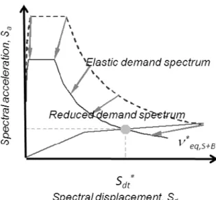
Figure 8.6 Variation of the total equivalent viscous damping with the spectral displacement Sd. At the p.p., Veq,S+B=19% for the retrofitted structure and Veq,S =11% for the existing building. ... 135

Figure 8.7 Modal mass participation for retrofitted structure ... 137

Figure 8.8 Modal shape configurations considering different control nodes: CM, DX, SX a) ϕ1,b) ϕ2, c) ϕ3, d) ϕ4 ... 138

Figure 8.9 P.P. for the CM is determined via CSM from original and reduced demand spectrum for the first mode Capacity spectra along Y direction ... 139

Figure 8.10 P.P. for the CM is determined via DCM ... 140

Figure 8.11 P.P. for the CM is determined via N2 ... 140

Figure 8.12 Pushover curves for the first significant three modes .. 141

Figure 8.13 P.P. for the CM is determined via CSM from original and reduced demand spectrum for the predominate modes along Y direction ... 142

Figure 8.14 P.P. obtained from different NSPs ... 142

Figure 8.15 Deformation of braces ... 143

Figure 8.16 Peak response for SX along Y direction ... 144

Figure 8.17 Peak response for CM along Y direction ... 145

(17)

Figure 8.19 normalized lateral load distributions ... 147

Figure 8.20 Effects of lateral load patterns ... 148

Figure 8.21 Force–displacement curves of BRBs ... 149

Figure 8.22 Capacity curves for CM ... 150

Figure 8.23 Construction MCC from the IMPA procedure. The P.P.mm is obtained by applying SRSS rule with the P.P. obtained from single mode pushover (Mode1..Mode n) and for each intensity level, repeat this procedure for a range of intensity levels (the response spectrum is scaled from lower to higher intensity levels and MCC can be obtained ... 151

Figure 8.24 the maximum base shear is asynchronous with the maximum roof displacement in the NL_RHA of TH1, the maximum roof displacement for the CM and maximum base shear is obtained to form the IDA curve ... 152

Figure 8.25 capacity curves obtained from different methods: the standard pushover analysis (for the predominate mode), IMPA method and IDA method for the left edge of building (SX) ... 153

Figure 8.26 capacity curves obtained from different methods: the standard pushover analysis (for the predominate mode), IMPA method and IDA method for the center of building (CM) ... 153

Figure 8.27 capacity curves obtained from different methods: the standard pushover analysis (for the predominate mode), IMPA method and IDA method for the right edge of building (DX) ... 154

Figure 8.28 Geometry of the original structure ... 155

Figure 8.29 Simulation of the initial imperfection of diagonal braces ... 156

(18)

Figure 8.30 P.P. is determined via CSM from original and reduced

demand spectrum for the first mode Capacity spectra ... 157

Figure 8.31 P.P. for the CM is determined from original and reduced demand spectrum for the first mode pushover curve ... 157

Figure 8.32 the axial force-displacement curve for BRBs ... 158

Figure 8.33 Geometry of the retrofitted structure ... 159

Figure 8.34 P.P. for diagonal braces in tension ... 160

Figure 8.35 P.P. for diagonal braces in compression ... 162

Figure 9.1 Force-displacement curves of viscous damper under various a ... 165

Figure 9.2 Force-displacement curves of viscoelastic damper ... 166

Figure 9.3 Force-displacement curves of metallic damper ... 168

Figure 9.4 Elevations of the existing structure ... 172

Figure 9.5 Plan view of the existing structure ... 172

Figure 9.6 Time history of the ground motions ... 173

Figure 9.7 Response spectrum curves under different earthquake waves ... 174

Figure 9.8 Analytical mode of the school building ... 176

Figure 9.9 Inter-story drift under minor earthquake ... 177

Figure 9.10 inter-story drift under major earthquake ... 177

Figure 9.11 Deign procedure for BRBs: performance points ... 179

Figure 9.12 Deign procedure for BRBs: Interstorey drifts ... 179

Figure 9.13 Optimization of BRBs ... 180

Figure 9.14 Elevation layout of the BRBs ... 182

Figure 9.15 Plan layout of the BRBs ... 182

(19)

Figure 9.17 Configuration of ADAS damper ... 184 Figure 9.18 Plan layouts of viscous or viscoelastic dampers ... 185 Figure 9.19 Plan layouts of ADAS dampers... 185 Figure 9.20 modal mass pacitipation: BRB designed through displacement base approach ... 187 Figure 9.21 modal shapes ... 188 Figure 9.22 Seismic response of the retrofitting structure under minor earthquake ... 190 Figure 9.23 Seismic response of the retrofitting structure under major earthquake ... 191 Figure 9.24 Maximum base shear ... 192 Figure 9.25 Location of the selected BRB to check the energy dissipation ... 193 Figure 9.26 Axial foece-displacement of the BRB designed through displacement based approach ... 194 Figure 9.27 Axial force-displacement of the BRB designed through force based approach ... 194 Figure 9.28 Axial force-displacement of the viscous damper designed through force based approach ... 195 Figure 9.29 Axial force-displacement of the ADAS damper designed through force based approach ... 195 Figure 9.30 Axial force-displacement of the Viscoelastic designed through force based approach ... 205 Figure 9.31 the internal force of the column ... 207

(20)

Tables index

Table 2.1Summary of studied NSPs ... 21

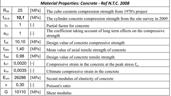
Table 5.1 Concrete properties ... 74

Table 5.2 Steel properties ... 75

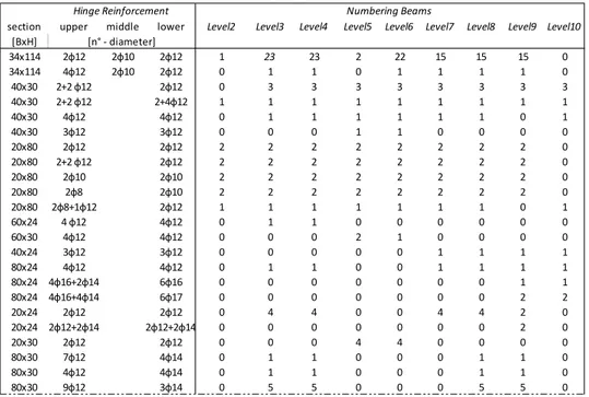
Table 5.3 Excerpt of variability of the sections and reinforcements beams at various levels ... 75

Table 5.4 Mass distribution for the structure ... 76

Table 5.5 the parameters defining the elastic spectrum ... 79

Table 6.1 P.P. obtained from DCM ... 87

Table 6.2 modal periods and participating mass ... 94

Table 6.3 SDF Parameters: Equivalent Elasto-Viscous system ... 99

Table 6.4 P.P. obtained from capacity spectra and capacity curve ... 99

Table 8.1 Parameters of dissipative braces for each floor ... 134

Table 8.2 Modal periods and participating mass for existing and retrofitted structures ... 136

Table 8.5 Parameters of BRBs ... 157

Table 9.1 Interstorey drift limit ... 175

Table 9.2 First six periods of the structure ... 175

Table 9.3 Shear forces and story drifts of time history analysis ... 180

Table 9.4 the parameters of the BRBs designed by two different approaches ... 181

(21)

Table 9.5 the parameters of the dampers ... 183 Table 9.6 Distribution of the Added Dampers ... 183 Table 9.7 First six periods of the structure ... 186

(22)

Symbol Index

m mass matrices of the system

c classical damping matrices of the system k lateral stiffness matrices of the system u floor displacement ι influence vector ( ) u t_g ground motion φ shape vector ut roof/top displacement

u* _{reference displacement of the SDOF system}

Vb Base Shear

ut Roof Displacement

Vy yield strength

Ke effective elastic stiffness

Ks hardening/softening stiffness α strain-hardening ratio

Teq initial period of the equivalent SDOF system

*

t

d trial peak deformation demand eq

ξ equivalent damping ratio

0

ξ inherent damping of the structure k a damping modification factor

h

ξ hysteretic damping

Γ modal participation factor

0

C the modification factor to relate spectral displacement of an equivalent SDOF system to the roof displacement of the building

1

C the modification factor to relate expected maximum inelastic

displacements to displacements calculated for linear elastic response

2

C the modification factor to represent the effect of pinched

hysteretic shape, stiffness degradation and strength deterioration on maximum displacement response

3

C the modification factor to represent increased displacements due to dynamic P-Δ effects

a

S the response spectrum acceleration at the effective fundamental

period and damping ratio (5% in this study) of the building e

T the effective fundamental period of the building in the direction under consideration

fs lateral force

sn modal inertia force distribution

n

w natural vibration frequency n

ξ _{the damping ratio for the nth mode}

qn(t) modal coordinate

(23)

st n

r modal static response

( ) n

D t _{movement of linear SDF system} i

F lateral load applied at floor level i i

m _{he floor mass}

i

h _{the story height}

k the period-dependent coefficient i

φ _{amplitude of the fundamental mode at level i}

i the floor number

j _{the mode number}

ij

φ _{amplitude of mode j at level i}

( , )

j j j

Sa ξ T the spectral acceleration at the periodTj

I0 diagonal matrix with I_{floor diaphragm} 0jj= I0j the polar moment of inertia of jth

a_λ _{non-negative scalar} λ _{scale factor (SF)}

1

a _{unscaled accelerogram}

ξni effective damping for nth mode

ξ0 the inherent damping of the elastic structure

Edni the energy dissipated in an ideal hysteretic cycle

Es0ni the maximum strain energy that the structure dissipates

Vbmmi multimodal base shear

urmmi multimodal roof displacement eq

ν equivalent viscous damping

,

'b j

K _{the elastic axial stiffness}

,

'b j

F _{the yield strength}

,

b j

β _{the hardening ratio}

b

θ _{the inclination of each brace}

Kb the horizontal components of stiffness

Fby the horizontal components of yield strength

Dby the horizontal components of displacement

δj the interstorey drift

νeq,s the equivalent viscous damping of the structure

ED,S the energy dissipated in a single cycle of amplitude D

ES,S the elastic strain energy corresponding to the displacement D

D the displacement reached from the structure ( )

s

F D _{the force corresponding to D (the force is the base shear)} sy

D _{displacement at yielding} sy

F _{the yielding force (base shear at yielding)}

,

bilinear D B

E the energy dissipated by the ideal hysteretic cycle of the

dissipative brace

(24)

χB corrective coefficient for the braces

νeq,S+B equivalent viscous damping of the braced structure

νI the inherent damping

, ,

bilinear D B j

E _{the energy dissipated by the dissipative braces placed at level j}

, ,

bilinear D B i

E the energy dissipated by the i braces placed at level j

νeq,S equivalent viscous damping provided by the original structure

νeq,B equivalent viscous damping provided by the braces

νtot total damping for the braced structure

K’b,j the equivalent stiffness of the spring series in the plastic range

K’p,j the equivalent stiffness of the spring series in the plastic range

Ad,j cross section of BRBs

fdy,j the yielding stress of the device

Ed,j the e elastic modulus of the device

ld,j the length of the device

VR the reference design life

PVR probability of exceedance of the seismic action

VN the nominal life

TR the return period

CN the importance coefficient

σ(Ti) the standard devisation of the response spectrums of the natutral

records in correspondence of the period Ti

Saj (Ti) the pseudo-acceleration of the jth spectrum

( )

a i

S T the mean pseudo-acceleration, N the number of the natural records

d

F the damping force of a single viscous damper

C the damping factor

v the velocity of the viscous damper

a damper parameter

K storage stiffness of the damper

β ratio of post stiffness

y

u the yield displacement

( )

Z t _{the evolutionary variable} F the story shearing force

(25)

1. Introduction

In recent years, as a result of seismic events occurred in Italy, the safety of buildings has become a topic of considerable interest. Therefore it is very important to develop fast and reliable analysis procedures to identify the safety level of existing structures.

The nonlinear dynamic time-history analysis is considered to be the most accurate method for the seismic assessment/design of structures. Nonlinear dynamic time-history analysis utilizes the combination of ground motion records with a detailed structural model, therefore is capable of producing results with relatively low uncertainty. In nonlinear dynamic analyses, the detailed structural model subjected to a ground-motion record produces estimates of component deformations for each degree of freedom in the model. Since the properties of the seismic response depend on the intensity, or severity, of the seismic shaking, a comprehensive assessment calls for numerous nonlinear dynamic analyses at various levels of intensity to represent different possible earthquake scenarios. This has led to the emergence of methods like the Incremental Dynamic Analysis.

Nonlinear dynamic time-history analyses are very time-consuming, which is a relevant drawback in design offices. Additionally the response derived from such an analysis is generally very sensitive to the characteristics of the ground motions as well as the material models used. All these render it quite impractical for everyday use, especially when overly complex structures need to be considered.

Nonlinear Static Procedures (NSPs) are deemed to be very practical tools to assess the nonlinear seismic performance of structures. In a pushover analysis, a mathematical model of the building, that includes all significant lateral force resisting members, is subjected to a monotonically increasing invariant (or adaptive) lateral force (or displacement) pattern until a pre-determined target displacement is reached or the building is on the verge of incipient collapse. Seismic design codes, like the FEMA273, FEMA356, FEMA440, ATC40 and Eurocode 8, have recommended the use of this type of procedures.

The use of NSPs for the seismic assessment of plan regular buildings and bridges is widespread nowadays. Their good performance in such cases is widely supported by the extensive number of scientific studies described in the previous studies.

(26)

However, capability of NSPs to closely correlate results from inelastic dynamic analysis has been checked with reference either to idealized building models or to geometrically simple tested structures. Real structures are almost always irregular as perfect regularity is an idealization that very rarely occurs. Structural irregularities may vary dramatically in their nature and, in principle, are very difficult to define. Actually, irregularity conditions in existing buildings can go far beyond the code definition of plan (and vertical) irregularity and, in any case, it is very likely that vertical and plan irregularities are combined. The use of NSPs in the case of real existing structures has so far been studied by a limited number of authors. This fact limits the application of NSPs to assess current existing structures.

Due to the development of NSP to evaluate the seismic demands of the structure, it is of a great interest to replace the NL_RHA for each given seismic intensity level by NSP to reduce the computational effort required for IDA. Remembering that MPA procedure retains the conceptual simplicity and computational attractiveness of current pushover procedures with invariant force distributions, it is of great interest to obtain capacity curves by replacing the nonlinear response history analysis of the IDA procedure with Modal Pushover Analysis (MPA). Another important use of NSPs is for the seismic retrofit of existing buildings. A displacement-based procedure to design dissipative bracings for the seismic protection of frame structures was proposed by Bergami & Nuti (2013): the procedure uses the capacity spectrum method, and no dynamic non linear analyses are needed. Two performance objectives have been considered developing the procedure: protect the structure against structural damage or collapse and avoid non-structural damage as well as excessive base shear. The compliance is obtained dimensioning dissipative braces to limit global displacements and interstorey drifts. In the design procedure, the capacity spectrum method is adopted to evaluate the seismic response of the existing or retrofitting buildings in terms of global displacement and interstorey drifts to evaluate the required equivalent viscous damping, valuate the additional equivalent viscous damping contribution due to the naked structure and braces, and check whether the insertion of the dissipative brace could make the structure satisfy performance requirement. In that paper, the procedure was validated through a comparison with nonlinear dynamic response of two 2D R.C. frames and a simple existing structure. In fact, frequently, the characteristics of an existing building (e.g. non regular distribution of

(27)

masses and stiffness, presence of a soft story) can compromise the effectiveness of procedures that impose a predefined loading pattern during pushover analyses. Moreover, in case of medium rise building (quite widespread in Italy), it is a matter of fact that the relevance of higher modes depends not only on their level of irregularity but also related to the quite high number of stories. To check such hypothesis of the design procedure has been tested on a medium rise irregular existing R.C. building in this work.

Another important issue in the procedure is the pushover curve in terms of base shear and roof displacement is taken as the capacity curve, and the intersection of capacity spectrum, which is transformed by the capacity curve, and demand spectrum is taken as the performance point (P.P.). There is big error for the capacity curve obtained from the monomodal pushover curve. Incremental dynamic analysis (IDA) is considered to be the most accurate method for the estimation of the seismic response and capacity of structures over the entire range of structural response, from elastic behavior to global dynamic instability. However, its intensive computation of many NL_RHA limits its practical use. It is necessary to improve the capacity evaluation for the structure in the design procedure. My work starts from the study of these problems and I tried to give a contribute on evaluating the accuracy of current NSPs on the seismic assessment of existing irregular structures, proposing a more efficient incremental modal pushover analysis (IMPA) to obtain capacity curve of the structure, incorporating IMPA into the design procedure of dissipative braces and its application to existing building. I studied these topics, I will describe the state of the art of NSPs, propose a more efficient incremental modal pushover analysis (IMPA) to obtain capacity curve of the structure, incorporate IMPA into the deign procedure of dissipative braces, a regular structure and an irregular structure are introduced and the current NSPs and IMPA are applied to these two buildings to check their accuracy, then the most accurate NSP and IMPA for the irregular structure are incorporated into the design procedure to retrofit the existing irregular structure, finally some other passive energy dissipation devices are selected to retrofit the existing irregular building to investigate their effectiveness.

1.1 Aims of the study

(28)

alternative to nonlinear response history analysis tools. Many international seismic design codes, like FEMA440, ATC40, Eurocode 8, Italian Technical Code NTC 2008 (NTC2008) and Chinese seismic code (GB 50011-2010) have recommended the use of this type of procedures. The use of NSPs is backed by a large number of extensive verification studies that have demonstrated their relatively good accuracy in estimating the seismic response of regular structures. The few studies on the extension of NSPs to the case of 3D irregular structures limit significantly the employment of NSPs to assess actual existing structures. In order to improve the use of NSPs in practical, the applicability of NSPs for analysis and retrofitting of existing buildings with dissipative braces should be checked. Therefore, the primary objectives of this work are: 1. Checking whether the commonly used procedures can be successful

even in the case of very complex irregularity conditions: Capacity Spectrum Method (CSM) adopted in ATC-40, Displacement Coefficient Method integrated into FEMA356, and N2 method presented in Eurocode 8 and modal pushover analysis (MPA).

2. Comparative evaluation of the different commonly used NSPs describing their advantages and limitations.

3. During the displacement based design procedure of dissipative braces, NSP is adopted to evaluate the seismic response of the existing and retrofitted structure, the applicability of NSPs to the case of braced irregular structures will be discussed. And The necessity of using a multi modal pushover instead of the standard single mode pushover in the design procedure has been investigated

4. Proposing a more efficient incremental modal pushover analysis (IMPA) to obtain capacity curve of the structure to evaluate the seismic demand: the procedure allows defining the capacity curve based on the execution of a series of MPAs.

5. Evaluating feasibility of force-based and displacement-based approaches for the design of passive energy dissipation devices and investigates the effectiveness of different passive energy devices.

1.2 Thesis layout

In chapter 2, the state of the art is reviewed. Four popular NPSs, which are Capacity Spectrum Method (CSM) adopted in ATC-40, Displacement Coefficient Method integrated into FEMA356, and N2 method presented in Eurocode 8 and modal pushover analysis (MPA), and the commonly

(29)

used lateral load distribution, are introduced. The development of extension of NSPs to 3D structure is presented.

In chapter 3, a more efficient incremental modal pushover analysis (IMPA) to obtain capacity curve of the structure to evaluate the seismic demand is proposed. The basic idea of IMPA is presented and the step-by-step computational procedure is summarized.

In chapter 4, a displacement-based procedure to design dissipative bracings for the seismic protection of frame structures is presented and the step by step procedure is summarized.

In chapter 5, the case studies used in this thesis and the modeling options assumed during the work are presented.

In chapter 6, the applicability of commonly used procedures to the very complex irregularity conditions is checked.

In chapter 7, IMPA is applied to existing building to evaluate seismic demand and capacity of structures over the entire range of structural response.

In chapter 8, the design procedure of dissipative bracings for the seismic protection of frame structures is applied to existing irregular structure and steel concentric braced frames (CBF).

In chapter 9, force-based and displacement design procedure of passive energy dissipation devices are applied to retrofit a school building located in shanghai, the comparisons of the two design methods and the seismic behavior of the retrofitting structure with different passive energy dissipation devices are discussed.

At the end, conclusions of the work developed are drawn and future work is outlined.

(30)

2. State of the art: NSP

2.1 Introduction

It is well known that the most accurate method of seismic demand prediction and performance evaluation of structures is nonlinear time history analysis. It is usually considered to be ‘exact’ results to assessment or design problems. The properties of each structural element are properly modeled, including nonlinearities of the materials, with the analysis solution being computed through a numerical step by-step integration of the equilibrium equation:

mu+cu+ku=-m u (t)ι _g (2.1)

where m, c and k are the mass, classical damping, and lateral stiffness matrices of the system; each element of the influence vector ι is equal to unity., and u (t)_g is the ground motion.

However, step-by-step integration demands a considerable computational effort and is very time-consuming; which is a relevant drawback especial in design phase.

During the last decade, the Nonlinear Static Procedure (NSP) analysis, often called Pushover Analysis, has been proposed among the structural engineering society as an alternative mean of analysis. The purpose of the pushover analysis is to assess the structural performance by estimating the strength and deformation capacities using static, nonlinear analysis and comparing these capacities with the demands at the corresponding performance levels.

In the pushover analysis, the structural model is subjected to a predetermined monotonic lateral load (forces or displacements) pattern, which approximately represents the relative inertia forces generated at locations of substantial mass. The intensity of the load is increased, i.e. the structure is ‘pushed’, and the sequence of cracks, yielding, plastic hinge formations, and the load at which failure of the various structural components occurs is recorded as function of the increasing lateral load. This incremental process continues until a predetermined displacement limit.

(31)

the force distribution and target displacement are based on the assumption that the response is controlled by the fundamental mode and that the mode shape remains unchanged after the structure yields. Obviously, after the structure yields both assumptions are approximate, but investigations (Saiidi and Sozen, 1981; Miranda, 1991; Lawson et al., 1994; Fajfar and Fischinger, 1988; Krawinkler and Seneviratna, 1998; Kim and D’Amore, 1999; Maison and Bonowitz, 1999; Gupta and Krawinkler, 1999, 2000; Skokan and Hart, 2000) have led to good estimates of seismic demands. However, such satisfactory predictions of seismic demands are mostly restricted to low- and medium-rise structures in which inelastic action is distributed throughout the height of the structure (Krawinkler and Seneviratna, 1998; Gupta and Krawinkler, 1999).

By assuming a single shape vector, {φ}, which is not a function of time and defining a relative displacement vector, u, of the MDOF system:

u= uφ t (2.2)

where ut denotes the roof/top displacement, the governing differential equation of the MDOF system will be transformed to:

m u +c u +k u =-m u (t)φ _t φ _t φ _t ι _g (2.3) If the reference displacement u* of the SDOF system is defined as

T * T m m t u φ φu φ ι = (2.4)

Pre-multiplying equation (1.3) by{φT

}, and substituting for ut using equation (2.3) the following differential equation describes the response:

T_{m u + c u + k u =- m u (t)}T T T t t t g φ φ φ φ φ φ φ ι (2.5) * *_{u + u + u =-}* * * * *_{u (t)} g M C K M (2.6) where *_{= m}T M φ ι (2.7) T * T T m = c m C φ φφ ι φ φ (2.8) T * T T m K = k m φ ι φ φ φ φ (2.9)

This provides the basis for transforming a dynamic problem to a static problem which is theoretically flawed. Furthermore, the response of a

(32)

Multi degree of freedom (MDOF) structure is related to the response of an equivalent Single degree of freedom (SDOF) system, ESDOF, as shown in Figure 2.1.

Figure 2.1Conceptual diagram for transformation of MDOF to SDOF system A nonlinear incremental static analysis of the MDOF structure can now be carried out from which it is possible to determine the force-deformation characteristics of the ESDOF system. The outcome of the analysis of the MDOF structure is a Base Shear, Vb, - Roof Displacement, ut, diagram, the global force-displacement curve or capacity curve of the structure,as shown in . This capacity curve provides valuable information about the response of the structure because it approximates how it will behave after exceeding its elastic limit. Some uncertainty exists about the post-elastic stage of the capacity curve and the information it can provide since the results are dependent on the material models used (Pankaj et al. 2004) and the modeling assumptions.

For simplicity, the curve is idealized as bilinear from which the yield strength Vy, effective elastic stiffness Ke and a hardening/softening stiffness Ks are defined. The idealised curve can then be used together with Eqs (2.4) and (2.9) to define the properties of the equivalent SDOF system, as shown in

Ks=αKe (2.10)

(33)

relationship of the ESDOF system is taken as the same as for the MDOF structure.

Thus the initial period Teq of the equivalent SDOF system will be: * * 2 eq M T K π = (2.11)

Figure 2.2(a) Capacity curve for MDOF structure, (b) bilinear idealization for the equivalent SDOF system.

The maximum displacement of the SDOF system subjected to a given ground motion can be found from either elastic or inelastic spectra or a time-history analysis. Then the corresponding displacement of the MDOF system can be estimated by re-arranging Eq. (2.4) as follows:

T * T m = m t u φ ι u φ φ (2.12)

The inelastic displacement of the controlled node (ut) is obtained by

making the correspondence of the target displacement of the SDOF system to the MDOF. In order to obtain the peak inelastic deformations of individual structural elements, such as interstorey drifts or chord rotations, one has to go back to the MDOF pushover curve step corresponding to the controlled node inelastic displacement previously calculated, and take the results in the desired elements.

The nonlinear static procedures can be classified as displacement-based evaluation methods for the assessment and rehabilitation of existing structures. However, these methods can be applied together with displacement-based design methods for the seismic design of new structures. In fact, to perform a pushover analysis it is necessary to

(34)

develop a nonlinear model of the structure, which includes the nonlinear formulation of the material relationships. In the case of reinforced concrete structures, the reinforcement in the elements must be correctly defined.

The main advantages of the nonlinear static analysis when compared with the linear dynamic and nonlinear dynamic analysis are listed below: 1) The seismic assessment and design using nonlinear static analysis are performed based on the control of structural deformations;

2) The NSPs explicitly consider the nonlinear behaviour of the structure instead of using the behaviour factors applied to the linear analysis results.

3) The nonlinear static analysis allows the definition of the capacity curve of the structure allowing the sequential identification of the structural elements that yield and collapse. This analysis identifies the structural damage distribution along the structure during the loading process, giving important information about the structural elements that first enter the inelastic regime which can turn out to be very useful when performing seismic strengthening of the structure;

4) The nonlinear static analysis is very useful within the performance based design and assessment philosophy, because it allows the consideration of different limit states and the performance check of the structure for the corresponding target displacements.

2.2 Pushover analysis methods

The use of nonlinear static procedures for the seismic assessment of planar frames and bridges has become very popular amongst the structural engineering community. The reason for their success lies in the possibility of gaining an important insight into the nonlinear seismic behaviour of structures in a simple and practical way.

The popular conventional pushover methods are the capacity spectrum method (CSM), Displacement Coefficient Method (DCM), N2 method and modal pushover analysis (MPA). The conventional pushover methods were officially introduced in design codes all over the world. They started to be implemented within the framework of performance-based seismic engineering ATC40, FEMA237 and FEMA356. Recently, the Japanese structural design code for buildings has adopted the capacity spectrum method (CSM) of ATC40 as a seismic assessment tool. In Europe, the N2 method was implemented in Eurocode 8.

(35)

2.2.1 Capacity Spectrum Method (CSM)

The Capacity Spectrum Method (CSM) was initially proposed by Freeman (1998) and later included in ATC-40 guidelines (ATC, 1996). This method compares the capacity of a structure to resist lateral forces to seismic demand given by a response spectrum. The response spectrum represents the demand while the pushover curve (or the “capacity curve”) represents the available capacity.

The capacity spectrum method is a very practical tool in the evaluation and retrofit of existing concrete buildings. Its graphical representation allows a clear understanding of how a building responds to an earthquake. The CSM was developed to represent the first mode response of a structure based on the idea that the fundamental mode of vibration is the predominant response of the structure. For buildings in which the higher mode effects can be important, the results obtained with the CSM may not be so accurate. A step-by-step summary of the CSM procedure to estimate the seismic demands for building is briefly described following, and the detailed procedure can be found in Appendix A.

1) Perform pushover analysis and determine the capacity curve in base shear (V_b) versus roof displacement of the building (D)； 2) Convert the capacity curve to acceleration–displacement terms

(AD) using an equivalent Single Degree of System (SDOF);

3) Plot the capacity spectra on the same graph with the 5%-damped elastic response spectrum that is also in AD format;

4) Select a trial peak deformation demand *

t

d and determine the

corresponding pseudo-acceleration from the capacity spectrum, initially assumingξ =5%;

5) The equivalent damping ratio ξ_eqcorresponding to *

t

d is evaluated

from the following relationship form: 0

eq k h

ξ = +ξ ξ (2.13)

where ξ is inherent damping of the structure, k is a damping ₀ modification factor that depends on the hysteretic behavior of the system, and ξ is the hysteretic damping. h

6) Update the estimate of *

t

d using the elastic demand spectrum for

eq

(36)

7) Check for convergence the displacement *

t

d . When convergence

has been achieved the target displacement of the MDOF system is equal to d_t:

*

t t

d = Γ d (2.14)

where Γ is the modal participation factor.

2.2.2 Displacement Coefficient Method (DCM)

When DCM is implemented, the target displacement, which is the displacement during a given seismic event of a characteristic node on the top of a structure, typically in the roof, is defined with the following formula: 2 0 1 2 3 ₄ 2 e t a T d C C C C S g π = (2.15)

where C0is the modification factor to relate spectral displacement of an equivalent SDOF system to the roof displacement of the building; C₁ is the modification factor to relate expected maximum inelastic displacements to displacements calculated for linear elastic response; C2 is the modification factor to represent the effect of pinched hysteretic shape, stiffness degradation and strength deterioration on maximum displacement response; C₃ is the modification factor to represent increased displacements due to dynamic P-Δ effects; Sa is the response

spectrum acceleration at the effective fundamental period and damping ratio (5% in this study) of the building in the direction under consideration; and T_eis the effective fundamental period of the building in the direction under consideration.

2.2.3 N2 method

The N2 method was initially proposed by Fajfar (1988, 1996) and was later expressed in a displacement-acceleration format (1999). And, the method has been included in the Eurocode8 (2004).

The basis of the method came from the Q-model proposed by Saiidi and Sozen (1981), which was improved by Fajfar and Gaspersic (1996). The N2 method was extended to bridges in 1997 (Fajfar. etc, 1997). In 1999, the N2 method was formulated in the acceleration-displacement format ((Fajfar, 1999), which combines the advantages of the graphical

(37)

representation of the capacity spectrum method developed by Freeman with the practicality of inelastic demand spectra. The method is actually a variant of the capacity spectrum method based on inelastic spectra.

Conceptually the method is a variation of CSM that instead of highly damped spectra using an R_μ − −μ T relationship. This method, as implemented in EC8, consists of the following steps:

1) Perform pushover analysis and obtain the capacity curve in

b

V −Dterms;

2) Convert the pushover curve of the MDOF system to the capacity diagram of an equivalent SDOF system and approximate the capacity curve with an idealized elasto-perfectly plastic relationship to get the period Te of the equivalent SDOF

3) The target displacement is then calculated: * _{( )[} _]2 2 e et a e T d S T π = (2.16)

where S Ta( )e is the elastic acceleration response spectrum at the

period T_e.

To determine the target displacement *

t

d , different expressions are suggested for the short and the medium to long-period ranges ,thus:

z *

C

T <T (short period range): If *_/ * _{( )}

y a e

F m ≥S T , the response is elastic and thus * *

t et

d =d . Otherwise the response is nonlinear and the ESDOF maximum displacement is calculated as * * et_{[1 (} ₁₎ C_] t e d T d R Rμ μ T = + − . z * C

T ≥T (medium and long period range):The target displacement of the inelastic system is equal to that of an elastic structure, thus * *

t et

d =d .

4) The displacement of the MDOF system is always calculated as *

t t

d = Γ . d

2.2.4 Modal Pushover Analysis (MPA)

None of the invariant force distributions can account for the contributions of higher modes to response, or for a redistribution of inertia forces

(38)

because of structural yielding and the associated changes in the vibration properties of the structure. To overcome these limitations, several researchers have proposed adaptive force distributions that attempt to follow more closely the time-variant distributions of inertia forces (Fajfar and Fischinger, 1988; Bracci et al., 1997; Gupta and Kunnath, 2000). While these adaptive force distributions may provide better estimates of seismic demands (Gupta and Kunnath, 2000), they are conceptually complicated and computationally demanding for routine application in structural engineering practice.

Chopra and Goel (2002) proposed an improved pushover analysis procedure based on structural dynamics theory, which retains the conceptual simplicity and computational attractiveness of current procedures with invariant force distribution. In this modal pushover analysis (MPA), the seismic demand due to individual terms in the modal expansion of the effective earthquake forces is determined by a pushover analysis using the inertia force distribution for each mode. Combining these ‘modal’ demands due to the first two or three terms of the expansion provides an estimate of the total seismic demand on inelastic systems. This procedure has been improved, especially in its treatment of P-Δ effects due to gravity loads, by including them in all modes. The improved version of MPA is summarized in Goel and Chopra (2004). This improved accuracy is achieved without any significant increase in computational effort. The MPA procedure estimates seismic demands much more accurately than current pushover procedures used in structural engineering practice (Goel and Chopra 2004, Chopra and Chintanapakdee 2004, Chopra,etc, 2004).

For each structural element of a building, the initial loading curve can be idealized appropriately (e.g. bilinear with or without degradation) and the unloading and reloading curves differ from the initial loading branch. Thus, the relations between lateral forces fs at the N floor levels and the

lateral displacements u are not single-valued, but depend on the history of the displacements:

(u,signu)

s s

f = f (2.17)

With this generalization for inelastic systems, Eq. (2.1) becomes:

mu+cu+ (u,signu)=-m u (t)fs ι g (2.18)

The standard approach is to directly solve these coupled equations, leading to the ‘exact’ non-linear RHA.

(39)

earthquake forces:

( ) - ( )

eff g

P t = m u tι (2.19)

The spatial distribution of these effective forces over the height of the building is defined by the vector s=mιand their time variation by ( )u t . _g

This force distribution can be expanded as a summation of modal inertia force distribution sn: 1 1 N N n n n n n mι S mφ = = =

∑

=

∑

Γ (2.20) , T , T n n n n n n n L L m M m M φ ι φ φ Γ = = = (2.21)

Although classical modal analysis is not valid for inelastic systems, it will be used next to transform Eq.(2.18) to the modal coordinates of the corresponding linear system. Each structural element of this elastic system is defined to have the same stiffness as the initial stiffness of the structural element of the inelastic system. Both systems have the same mass and damping. Therefore, the natural vibration periods and modes of the corresponding linear system are the same as the vibration properties of the inelastic system undergoing small oscillations (within the linear range).

Expanding the displacements of the inelastic system in terms of the natural vibration modes of the corresponding linear system, we get

1 (t) N _{n n}(t) n u φ q = =

∑

(2.22)

Substituting Eq. (2.23) into Eq. (2.18), pre-multiplying by φnT, and using the mass and classical damping orthogonality property of modes gives: 2 sn - ( ), 1, 2,..., n n n n n g n F q w q u t n N M ξ + + = Γ = (2.23) ( , ) T ( , ) sn sn n n n s n n F =F q signq =φ f u signu (2.24)

where wn is the natural vibration frequency and ξ is the damping ratio n

for the nth mode.

1. UNCOUPLED MODAL RESPONSE HISTORY ANALYSIS

Neglecting the coupling of the N equations in modal coordinates leads to the uncoupled modal response history analysis (UMRHA) procedure. This approximate RHA procedure is the preliminary step in developing a

(40)

modal pushover analysis procedure for inelastic systems.

The spatial distribution s of the effective earthquake forces is expanded into the modal contributionss_n, where φn are now the modes of the corresponding linear system. The equations governing the response of the inelastic system to peff,n (t ) given by:

2 sn - ( ), 1, 2,..., n n n n n g n F q w q u t n N M ξ + + = Γ = (2.25)

This resisting force depends on all modal coordinates qn(t), implying coupling of modal coordinates because of yielding of the structure. The solution qn of Eq.(2.25) is given by:

( , ) - ( ) s n g mu cu+ + f u signu = s u t (2.26) ( ) ( ) n n n q t = Γ D t (2.27)

where D tn( ) is governed by the equation of motion for the nth-mode

linear SDF system, an SDF system with vibration properties—natural frequency wnand damping ratio ξ —of the nth-mode of the MDF n

system, subjected to u t : _g( ) 2 sn - ( ) n n n n g n F D w D u t L ξ + + = (2.28) ( , ) T ( , ) sn sn n n n s n n F =F D signD =φ f D signD (2.29)

Substituting Equation (2.27) into Equation (2.24) gives the floor displacements

( ) ( )

n n n n

u t = Γ φ D t (2.30)

Any response quantity r(t)—storey drifts, internal element forces,

etc.—can be expressed as ( ) st (t) n n n r t =r A (2.31) where st n

r denotes the modal static response, the static value of r due

to external forcess_n, and

2 (t)=

n n n

(41)

a) Static Analysis of Structure

b) Dynamic Analysis of Inelastic SDF System Figure 2.3 Conceptual explanation of uncoupled modal response history analysis of

inelastic MDF systems

Solution of the nonlinear Eq. (2.29) formulated in this manner provides

Dn (t) , which substituted into Eq. (2.30) gives the floor displacements of the structure associated with the nth-“mode” inelastic SDF system. Any floor displacement, story drift, or another deformation response quantity r

(t) is given by Eqs. (2.13) and (2.14), where An(t) is now the

pseudoacceleration response of the nth-“mode” inelastic SDF system. The two analyses leading to st

n

r and An(t)are shown schematically in Fig. 4.3.

Eqs. (2.13) and (2.14) represent the response of the inelastic MDF system to peff (t ), the nth-mode contribution to peff (t ) . Therefore the response of the system to the total excitation peff (t ) is given by Eqs. (2.15) and (2.16). This is the UMRHA procedure.

What is an appropriate invariant distribution of lateral forces to determine

Fsn? For an inelastic system no invariant distribution of forces can produce displacements proportional to φ at all displacements or force _n levels. However, before any part of the structure yields, the only force distribution that produces displacements proportional to φ is given by Eq. _n (2.22). Therefore, this distribution seems to be a rational choice—even

(42)

after the structure yields—to determine Fsn in Eq. (2.22). When implemented by commercially available software, such non-linear static analysis provides the so-called pushover curve, which is different than the

Fsn/Ln–Dn curve. The structure is pushed using the force distribution of Eq. (2.22) to some predetermined roof displacement, and the base shear Vbn is plotted against roof displacement urn. A bilinear idealization of this pushover curve for the nth-‘mode’ is shown in Figure 2.4 a). At the yield point, the base shear is Vbny and roof displacement is urny. How to convert this Vbn–urn pushover curve to the Fsn/Ln–Dn relation? The two sets of forces and displacements are related as follows:

, bn rn sn n n n rn V u F D φ = = Γ Γ (2.33)

Eq.(2.33) enables conversion of the pushover curve to the desired

Fsn/Ln–Dn relation shown in Figure 5(b), where the yield values of Fsn/Ln relation and Dn are

*,

sny bny rny

ny n n n rn F V u D L = M =Γφ (2.34) in which * n

M is the effective modal mass:

*

n n n

M = ΓL (2.35)

The two are related through

2 sny n ny n F w D L = (2.36)

implying that the initial slope of the bilinear curve in Figure 2.4 b) is 2

n

w .Knowing Fsny/Ln and Dny from Eq. (2.24), the elastic vibration period

Tn of the nth-‘mode’ inelastic SDF system is computed from 2 2 ( n ny) n sny L D T F π = (2.37)

(43)

a) idealized Pushover Curve

b) Fsn/Ln–Dn relation

Figure 2.4Properties of the nth-“mode” inelastic SDF system from the pushover curve

3. Modal pushover analysis

A pushover analysis procedure is presented next to estimate the peak response rno of the inelastic MDF system to effective earthquake forces

(44)

lateral forces distributed over the building height according to sn, with the structure is pushed to the roof displacement urno. This value of the roof displacement is given by Eq. (2.21) where Dn, the peak value of Dn (t ) , is now determined by solving Eq. (2.28); alternatively, it can be determined from the inelastic response (or design) spectrum (Chopra, 2001; Sections 7.6 and 7.12). At this roof displacement, the pushover analysis provides an estimate of the peak value rno of any response rn(t): floor displacements, storey drifts, joint rotations, plastic hinge rotations, etc.

This pushover analysis, although somewhat intuitive for inelastic buildings, seems rational for two reasons. First, pushover analysis for each ‘mode’ provides the exact modal response for elastic buildings and the overall procedure, as demonstrated earlier, provides results that are identical to the well-known RSA procedure. Second, the lateral force distribution used appears to be the most rational choice among all invariant distribution of forces.

The response value rno is an estimate of the peak value of the response of

the inelastic system to peff,n(t), governed by Eq. (2.26). As shown earlier for elastic systems, rno also represents the exact peak value of the

nth-mode contribution rn(t) to response r(t). Thus, we will refer to rno as the peak ‘modal’ response even in the case of inelastic systems. The peak ‘modal’ responses rno, each determined by one pushover analysis, is combined using an appropriate modal combination rule, e.g. Eq. (2.17), to obtain an estimate of the peak value ro of the total response. This application of modal combination rules to inelastic systems obviously lacks a theoretical basis. However, it provides results for elastic buildings that are identical to the well-known RSA procedure described earlier.

2.3 Summary of NSPs

Table 2.1 shows a summary of the methods used in this work pointing out the main differences between the methods in each step of the nonlinear static procedure.