Control architectures for heterogeneous fleets of unmanned vehicle systems

(1)

UNIVERSITÀ DEGLI STUDI DI CATANIA

FACOLTÀ DI INGEGNERIA ELETTRICA ELETTRONICA E

INFORMATICA

XXVII cycle Ph.D. in System Engineering

Antonino Catena

Control Architectures for Heterogeneous Fleets of

Unmanned Vehicle Systems

Ph.D. Thesis

Tutor: Prof. G. Muscato Coordinator: Prof. L. Fortuna

(2)

(3)

Preface | I

Preface

The field of aerial robotics, from 20 years ago up to now, has had an incredible growth. The reasons are several, but surely, the key motivation is the development of MEMS sensors and microcontroller more and more cheap and reliable. The “Dipartimento di Ingegneria Elettrica, Elettronica e Informatica” (DIEEI) at the University of Catania is involved in several research projects focused on the study and development of Unmanned Aerial Systems (UASs).

The most well-known project of DIEEI in the field of Unmanned Aerial Vehicles (UAVs) is the Volcan Project, an autonomous aerial platform for volcano activities monitoring in order to analyze gases and to improve the forecast of the lava flow during an eruption.

In addition to the Volcan project, many research activities of DIEEI are focused on problematic related to UAVs that nowadays are still open, such as cooperation with different type of robotic platforms, inertial navigation, visual navigation and last but not least, the power management in order to maximize the autonomy. This Ph.D. course was related to and funded by the Ambition Power project [64], whose objective was the virtual prototyping of power devices in avionics field.

(4)

Acknowledgements

First of all, I would like deeply thank my family: had it not been for them, nothing would have been possible.

My very special thanks go to my Tutor Prof. Eng. Giovanni Muscato, who believed in me, gave me the possibility to demonstrate my capabilities, supported me with his scientific knowledge, and to the Ph.D. Coordinator Prof. Eng. Luigi Fortuna, because he worked as a real team manager, defending and motivating our group.

I would also like to thank the members of the Service Robots Group for their being helpful, patient and sapient: Eng. Donato Melita, Eng. Luciano Vito Cantelli, and Prof. Domenico Longo.

Last but not least, a particular thanks to my Ph.D. colleagues: Viviana, Davide e Marco, because they have contributed to make these three years unforgettable.

(5)

Nomenclature | III

Nomenclature

ACI: AscTec Communication Interface ACK: Acknowledgement

ADAHRS: Air Data and Attitude Heading Reference System ADC: Analog to Digital Converter

AGATE: Advanced General Aviation Transport Experiment AoA: Angle of Attack

ASL: Above Sea Level

AUV: Unmanned Underwater Vehicle CAN: Controller Area Network

CSMA/CD: Carrier Sense Multiple Access with Collision Detection DIEEI: Dipartimento di Ingegneria, Elettrica, Elettronica ed Informatica DLL: Dynamic Link Library

DoF: Degree of Freedom DSD: Debug Service Data EAP: Electro-Active Polimer EKF: Extended Kalman Filter

ENAC: Ente Nazionale Aviazione Civile

EEPROM: Electrically Erasable Programmable Read-Only Memory FCCS: Flight Control Computer System

FW: FirmWare

GPS: Global Positioning System GUI: Graphical User Interface HIL: Hardware In the Loop HL: High Level (processor) HMI: Human Machine Interface I2_{C: Inter Integrated Circuit}

ICAO: International Civil Aviation Organization IDE: Integrated development environment IMU: Inertial Measurement Unit

LiPo: Lithium Polymer LL: Low Level (processor) LTA: Light then Air

(6)

MEMS: Micro Electro Mechanical Systems

NASA: National Aeronautics and Space Administration NOD: Normal Operation Data

NSH: High-priority Node Service Data ODR: Output Data Rate

OS: Operating System PCB: Printed Circuit Board PIC: Pilot in Command ROR: Route Of Robot RPA: Remotely piloted aircraft RPV: Remotely Piloted Vehicle RPY: Roll Pitch Yaw

RS-232: Recommended Standard 232 RTK: Real Time Kinematic

S&R: Search and Rescue

SACS: Servo Actuators Control System SDK: software development kit

SLAM: Simultaneous Localization And Mapping SNR: Signal Noise Ratio

SoA: State of Art

SPI: Serial Peripheral Interface SWD: Serial Wire Debug UAV: Unmanned Aerial Vehicle UDP: User Datagram Protocol UGV: Unmanned Ground Vehicle

USART: Universal Synchronous-Asynchronous Receiver/Transmitter USB: Universal Serial Bus

UVS: Unmanned Vehicle System VI: Virtual Instrument

VTOL: Vertical TakeOff and Landing WP: WayPoint

(7)

Contents | V

Chapter I. Introduction

I.1 The State of the Art

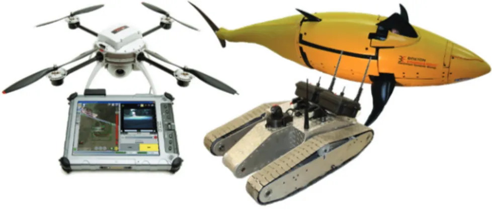
The adoption of UVSs (Unmanned Vehicle System) as performing tools to be used for data gathering, S&R operations, civil protection and safety issues is rapidly increasing. Generally, the unmanned vehicles are grouped in three categories:

• UAV, Unmanned Aerial Vehicles • UGV, Unmanned Ground Vehicles • AUV, Autonomous Underwater Vehicles

Figure 1 - Examples of UVSs

The topic of this thesis is strictly related to the first class of robots, which are the robotic platforms able to fly without pilot.

I.1.1 Normative: UAV, RPA or RPV?

The increasingly frequent use of drones in recent years [2] [3] has made it essential a legislation concerning them in order to regulate its use. There is a general legislation drafted by ICAO [15], the International Civil Aviation Organization, whereas as regards the UAVs with a weight less than 150 Kg there is a particular normative depending by the nation. In the case of Italy, this

(14)

normative is drafted by the ENAC [14]. The key aspect of the normative is that the use of a completely autonomous robotic platform in open field is illegal, except for very particular cases that, however, require permission by the relevant authorities. In fact, according to normative, there must be someone that pilots, or in general supervises, the aircraft. For this reason, the relevant authorities prefer using the terms such as Remotely Piloted Vehicle (RPV) or Remotely Piloted Aircraft (RPA) in place of UAV, in order to underline the role, and the responsibilities, of the operator that controls the plane, which, according to the normative, is to all effects a pilot. Moreover, still according to the law, anyone who pilots a drone must have a license, issued after an examination, and an insurance that covers the risks connected with the activity of the drone.

I.1.2 Classification of UAVs

To make a complete summary of all the models of UAV is a really difficult operation, because of the huge variety of applications in which they are used. On the other hand, it's possible to make a comparison between them, on the basis of particular aspects, such as dimension, airframe and scope [1].

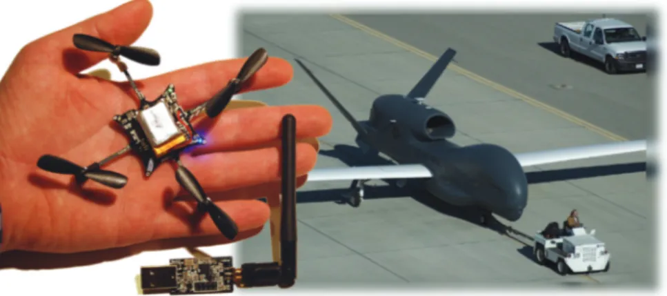
I.1.2.1 UAV Dimension

A first comparison between UAV takes into account their dimension, and then their mass (Figure 2). As it is shown in the following table, the mass of a drone is strictly connected to its autonomy and operational range.

Category Acronym Mass[Kg] Max Op. _Range[Km] Max Flight _Altitude[m] Max Duration _{of Flight[h]} Nano η <0.0250 1 100 0.5 Micro µ <5 10 250 1 Mini Mini <30 10 300 2 Close Range CR <150 30 3000 4 Short Range SR <200 70 3000 6 Medium Range MR <1250 200 5000 10

(15)

Figure 2 - Different dimensions of UAVs

I.1.2.2 UAV Airframes

Essentially, the airframe of an UAV may be of five different types. It is worth to point out that there isn't "the best one" airframe for every application, but each airframe has advantages and disadvantages, which must be evaluated, in order to choose the best drone to accomplish a given task.

Fixed wings

This is the most common airframe for big drones, especially for the maturity of technology (Figure 3). This type of airframe gives great advantages in terms of efficiency and power consumption, due to the additional lift provided from the wings. However, the wings require a minimum speed cruising to perform their tasks. This aspect brings to the main limit of this type of airframe: the incapability to hover or fly slower, in addition to the fact that they require a runway for takeoff and landing operations. For these reasons they are unsuitable for indoor applications.

(16)

Figure 3 - Fixed wings airframe

Rotary wings

This class of airframe gets the necessary lift to fly directly by the propellers. Moreover, they are able to hover and to execute vertical takeoff and landing (VTOL). This makes them perfect for indoor flight. Depending on propellers number, it is possible to split this class in two groups:

• Helicopters: this type of airframe has one or two rotors (Figure 4). In relation to this class of aircraft, this structure ensures the best performance in terms of energy consumption. In fact, the rotor has a practically constant speed and the aircraft movements are given by the variation of the angle of attack (AoA) of the blades. In a few words, the speed of a helicopter is not related to the speed of rotation of the rotor, but essentially to the AoA of the blades. Anyhow, such a rotor is a very complex system (Figure 5) and, even if its technology is consolidated, this has an impact on the cost and reliability.

(17)

Figure 5 - Helicopter rotor

• Multirotors: to this group belongs airframes that have three or more (generally, up to eight) rotors (Figure 6). With respect to helicopters, in these drones the propellers have a fixed AoA, but variable speed. This means a great simplicity in the mechanical structure, but a worst power management. It is precisely the mechanical simplicity that has made the multirotors the most common airframes for small drones, especially in the field of academic research.

Figure 6 - Multirotors airframe

Tilt rotors

This class of airframes is a hybrid between the two previously discussed configurations (Figure 7). Such a structure is capable, at the same time, to execute vertical takeoff and landing, to stay in hovering and to reach a cruise speed comparable with a fixed wings system. However, it is important to underline that these features are achieved by means the rotation of the rotors, which causes reliability problems and a very complex control during the transition phase. In

(18)

addition, another disadvantage of this airframe resides in the propellers: a propeller designed for the hovering is not optimized for flying, and viceversa. In other words, a tiltrotor is capable to hover, but it is worst with respect to a rotary wing. Moreover it is capable to fly forward for a long range, but consuming more energy respect to a fixed wing.

Figure 7 - Tiltrotor airframe

Flapping wings

This bio-inspired UAV airframe is the most recent. Its main limit, in fact, derives from the fact that the technology behind it is not mature yet. There are still open issues: ignoring for now problems related to control, probably the most interesting challenge regards the development of linear actuators, capable to reproduce the muscle motion. A possible solution could be the electro-active polymers (EAP), but this is not yet a mature technology and some years are still needed to obtain a commercial product. Depending on the animal to which they are inspired, there are two classes of flapping wings airframes:

• Ornithopters: bird-like airframes, which generate lift by flapping wings up and down with synchronized small variations of AoA (Figure 8). As in the fixed wings airframes, this type of flapping wings requires a forward flight to generate lift.

• Entomopters: inspired to the insect structure, this airframe generates a great variation of AoA between the upstroke and the downstroke phases (Figure 9). Unlike the previous one, this airframe is capable to hover and to execute vertical takeoff and landing.

(19)

Figure 8 - Flapping wings, bird-like airframe

Figure 9 - Flapping wings, insect-like airframe

Blimp

To this last class of airframe belong drones called Lighter Than Air, or LTA (Figure 10). It is easy to guess how this airframe has the best efficiency in terms of energy, since no energy is needed to hover. However, generally these airframes move slower than the other types of airframes, have a bigger volume, in order to obtain enough lift force and, above all, have a limited payload. The latter peculiarity represents the biggest disadvantage of this type of airframe, because a typical mission with a drone often requires additional equipment such as cameras, sensors, robotic arms and so on.

(20)

Figure 10 - LTA airframe

To summarize, in Table 2 the main features of each airframe are compared.

Fixed Wings Rotary Wings Tilt Rotors Flapping Wings Blimp Power efficiency Medium Bad Bad Medium Good

Control Good Good Medium Bad Good

Miniaturization Medium Good Bad Medium Bad

Payload Good Medium Good Bad Bad

Hover Bad Good Medium Medium Good

Low Speed Fly Bad Good Medium Medium Good

High Speed Fly Good Bad Medium Bad Bad

Robustness Good Medium Bad Bad Bad

Maneuverability Medium Good Medium Bad Good

Indoor usage Bad Good Bad Bad Medium

Outdoor usage Good Medium Medium Medium Good

Table 2 - UAV airframes comparison

I.1.2.3 Scope

In the last years the number and the diversity of applications regarding the use of UAVs is increased enormously. A first distinction is usually made between military and civil applications. Focusing on the second group, the non-military applications where the UAVs are commonly used are:

• Disaster management [4] [5].

• Agricultural monitoring and management [6]. • Infrastructure inspection [7] [8].

• Law enforcement [9]. • Weather monitoring.

• Environmental monitoring and exploration [10] [11] [12]. • Aerial imaging/mapping.

(21)

• Entertainment: television news coverage, sporting events, moviemaking. • Freight transport.

• Oil and gas exploration [13].

As regards the DIEEI [52], the research activities are focused mainly on monitoring and forecasting of volcanic activity. The volcano under examination is the Mount Etna, one of the most active volcanoes in the world, which is in an almost constant state of eruption. In the next chapter the developed UAV, i.e. the Volcan, will be treated.

(22)

I.2 Architecture of an UAV

The design of an UAV control system is a very complex mission and, as it often happens in engineering topics, there is no a single way to accomplish this task. Listing all the possible architectures goes beyond the scope of the thesis, therefore in the next chapters we will focus only on the control architectures of the UAVs used. However, some milestones are always present in the development of an UAV control system.

The choice of the model

This is the first and probably the most important step. A good modeling represents the key phase in order to obtain satisfactory dynamic performances. The expression "good modeling" is not intended as a perfect modeling, where every dynamic effect is considered, but as a modeling where only the most important dynamic modes are taken into account.

The control strategies

Once the model has been developed, it is necessary to ensure the system stability and, as far as possible, the immunity to noise and to unmodeled dynamics. The most used control strategies use PID [17] controllers or digital filters such as EKF [40] [41] and complementary filters [42] [43]. Once the stability is obtained, the next step is focusing on high level control tasks such as collision avoidance, cooperation, fault detection and so on.

Sensors

Sensors are fundamental in order to obtain information about the state of the drone. As regards the stability, an Inertial Measurement Unit (IMU) is needed. This system returns roll and pitch resulting by a sensors fusion of a three axial accelerometer and of a three axial gyroscope. Often a three axial magnetometer is added in order to obtain also the yaw angle. For navigation, generally GPS and pressure sensors are used. Finally, for high level tasks as obstacle avoidance or object tracking, cameras, laser scanners and ad hoc sensors are used. For the choice of the sensors, in addition to the precision, the other parameters to take into account are the bandwidth, the power consumption, the immunity to noise and last but not least, the easy of interfacing to a microprocessor.

(23)

Architecture of an UAV | 11

Motors and actuators

Motors and actuators connected to the mobile parts of the drones are necessary to transduce the commands coming from control unit. As for the sensors, precision and bandwidth are important parameters to consider in their choice. Moreover, it is extremely important to underline that this is the part of the whole architecture that consumes more energy. So, if in one hand more power means more torque, on the other hand it means more weight and less autonomy.

CPUs

The core of the control architecture computes data coming from sensors and in according to the task, sends commands to actuators. If to execute a stability control by means a set of PID controllers is adequate a commercial microprocessor that costs a few Euros, to accomplish complex tasks in real time such as SLAM or recognize a target by means of an HD camera it is necessary a dedicated PC with a real time OS. Also in this case it is mandatory the monitoring of the energy consumption, since the computational load of the control algorithm is strictly related to the energy necessary to execute it.

Communication Protocols

As discussed in the section I.1.1, for normative reason a drone always has to be connected to a remote station, where an operator can monitor and supervise its mission. Moreover, the control systems are becoming more and more complex and often they are realized as a combination of subsystems connected each other. For this reason the choice of the communication protocol is dual: to communicate to remote station and to interconnect the various subsystems of the control architecture. As regards the former, generally this link is used also to send the drone telemetry. In most cases this connection is made by a WiFi link. As concern the latter, is mandatory to choose a communication protocol that guarantees a data rate at least an order of magnitude greater than the bandwidth of the sensors and actuators used and also an SNR as small is possible. A differential communication with a good bandwidth, like the CANbus, is suitable for this purpose. However, generally also a normal serial communication could be suitable.

(24)

I.3 Limits and Challenges

From now on, this thesis will be focused exclusively on fixed wings and multirotors, i.e. those airframes mainly used for both civilian and research activities. As mentioned in the previous pages, the progress in this field has been enormous, especially in the last 5 years. However, there are still some aspects where some improvement and clarifications are needed. Probably, the key limitation resides on the current normative. If on the one hand, the scientific community tries to develop a completely autonomous UAV [2], on the other hand actual rules generally require a human supervisor responsible for the actions of the robot. Surely, this is a difficult aspect to solve and even if a normative exist, these are destined to be modified in accordance with the technological growth. As regards the technical aspect, the most evident bottleneck is the energy management. Generally, even if the energy density of the batteries has steadily increased during the last years, the autonomy of a commercial UAV with brushless motors is less than 30 minutes. This is a limit extremely incapacitating, when you consider a complex task to accomplish, such as mapping an area or search a target, which generally requires a lot of time. Moreover, a complex task requires a high computational load, which obviously consumes a lot of energy, further reducing the autonomy. At present, the most common batteries used are of LiPo type. A good alternative could be fuel cells, i.e. a sort of battery in which the fuel is transformed into electric current through an electrochemical process. However also fuel cells have an energy density lower than other sources, such as gasoline or methanol [1]. Increasing the autonomy of an UAV is without doubt the main challenge that the scientific community have to face in the next years. Concerning the control algorithms, the results so far are more than satisfactory, even if the best performance are generally obtained indoor, thanks to the feedback provided by motion detection systems, as the Vicon [59] . The ETH of Zurich [62] and the CATEC in Seville [63] are among the best European research centers in this field. However, to get a level of control comparable in outdoors conditions is a hard challenge. The main reasons are two:

• First of all, motion tracking systems are unsuitable for outdoor applications, in particular in the case of unstructured environments. Normally MEMS sensors are used, such as accelerometers, gyroscopes and magnetometers to help localization. These sensors are less precise and

(25)

Limits and Challenges | 13

noisier respect to a motion tracking system, and then the feedback of the control architecture is less reliable.

• Secondly, an unstructured environment introduces dynamics that degrade the accuracy of the mathematical model of the aircraft.

(26)

I.4 Development tools

The testing phase during the design of the control architecture of an UAV is the longest phase in terms of time. This is because, despite other robotics platform such as UGVs, a bug in the control algorithm most of the times means the destruction of the drone itself. A powerful method to test the control algorithm is the Hardware In the Loop (HIL) architecture [32] [33], where the real aircraft is substituted with a virtual one, generally within a flight simulator. In this way it is possible to test and tune the control architecture, under the assumption that the aircraft model of the flight simulator reflects satisfactorily the dynamic behavior of the real one. However, in HIL architecture it is not possible to test other fundamentals parts of the whole system, such as sensors and actuators. A step ahead in this direction is represented by the Motion Capture technique. In this scenario, the drone operates inside an arena, where a set of high speed cameras provide an extremely precisely feedback regarding pose and position. In this way, in addition to the control algorithm, it is possible to test the actuators and compare the telemetry coming from the sensors, with the other measurements one coming from the cameras. The only limitation in this case is that within the arena the environment is perfectly structured, so it is not possible to test the robustness of the control algorithm, i.e. its dynamic performance when the drone operates in noisy and not structured environments.

(27)

Objectives | 15

I.5 Objectives

In the previous paragraphs the UAV SoA was briefly presented, underlining as several research field are evolving. In particular, as regards the UAV features, it is clear as there isn't "a general purpose" drone, capable to accomplish whatever task. For this reason, a keyword in the next years for the researchers will be the cooperation between heterogeneous robotic platforms. More and more often complex tasks require features that a single drone doesn't have. For example, to patrol a huge area, it is required a drone suitable to fly forward with high speed, to be capable to hover and to have a good autonomy. In a few words, it is impossible for a single drone, but also for a homogeneous fleet.

From this consideration is born the objective of this thesis: to develop a fleet of heterogeneous UAV, composed by the following parts:

• A fixed wing aircraft, represented by the Volcan UAV [16].

• A quadrotor, represented by the Hummingbird produced by Asctec [60].

• A multiplatform HMI developed in LabView [48], in order to monitor and supervise the heterogeneous fleet.

The next chapters are organized in the following way: the second one describes the Volcan. The third chapter treats the Hummingbird by Asctec. The fourth chapter presents the HMI developed and finally, the last one discusses about the conclusions.

(28)

Chapter II. The Volcan UAV

II.1 Introduction

As mentioned before, the Volcan UAV is the fixed wing developed for the mission related to volcano monitoring. In order to accomplish missions in hard environments and conditions, the project designed is a V-tail fixed wings very similar to the famous Aerosonde [18] (Figure 11), with the following features:

• Fuselage in carbon fiber and fiberglass • Wooden wing and V-tail

• A wing span of 3m • A total weight of 13kg • A 2000W brushless motor

• A maximum cruise speed of 150km/h

Figure 11 - Volcan UAV

The choice to develop a fixed wing is given by the fact that on the Etna the weather conditions are really adverse, not to mention the reduction of the air density, which at 3000m reduces drastically the lift of the airframe. The use of an electric engine is given by two factors:

• First of all, because the reduced air density has a negative effect on the carburetion of a stroke engine.

• Secondly, gases produced by the motor would distort the measures of the gas sensors.

(29)

Introduction | 17

The Volcan has been entirely designed in the DIEEI laboratories. In particular, during this Ph.D. activity a new control architecture has been developed [17]. In the following sections the steps that have led to the development the whole system will be discussed.

II.1.1 System architecture overview

The core of the control architecture is based on the interaction between different sub-systems developed in DIEEI laboratories (Figure 12):

• ADAHRS, the Air Data and Attitude Heading Reference System, is the sensors board and manages all the sensors in order to compute the pose and the position of the vehicle

• SACS, the Servo Actuators Control System, controls the engine and the actuators connected to the mobile parts of the drone.

• FCCS, the Flight Control Computer System, receives data from the sensors and, according with the flight plan, sends commands to the interface board.

• UDP2CAN, the data link board, connects the drone with a remote station, in order to send telemetry and to permit to the operator to supervise it.

Figure 12 - Volcan control system

The whole architecture has been divided in various subsystems in order to maximize flexibility and modularity.

(30)

II.2 CAN: Control Area Network

The different subsystems forming the UAV control system need to exchange data constantly. Therefore it is necessary to use a communication protocol which gives wide guarantees of reliability and immunity to noise, moreover with a bandwidth such as to permit a real-time control of the drone. For these reasons the CANbus protocol (Controller Area Network) was chosen. CANbus is a broadcast serial bus, introduced by Bosch in the early 80s [19]. Initially designed for automotive applications, now the CANbus is used in many industrial sectors, including avionics. Its success is due to the considerable technological advantages it offers:

• Rigid Response time. This feature is fundamental for the control process. • Simplicity and flexibility of wiring: the CAN is a serial bus which is

typically implemented on a twisted pair (shielded or not, depending on the requirements).

• Multi-Master architecture, where all nodes of the network can transmit and multiple nodes of the network can request to transmit data simultaneously. They are characterized by network addresses different by the conventional sense. In fact the messages are routed on the basis on the importance of the variable to be sent and not on the basis of the address of the transmitter. Each variable has an identifier, which indicates the priority for the access to the bus. Thanks to this peculiarity, the nodes don't have an address that identifies them, so in this way they can then be added or removed to the network without reorganizing it.

• High noise immunity: the standard ISO11898 [20] imposes that the transceiver chip can continue to communicate even in extreme conditions, such as the interruption of one of the two wires or short circuit of one of them with ground or with the power supply.

The transmission rate depends on the size of the maximum length of the bus (Figure 13). In case of short distances, as in the case under exam, it is possible obtaining a bit-rate up to 1Mbit/s

(31)

CAN: Control Area Network | 19

Figure 13 - CANbus data rate

II.2.1 Rules for bus access

In order to manage a multi-master architecture, the CANbus uses a modified CSMA/CD protocol, which uses the concept of dominant and recessive bits. When two or more nodes are transmitting simultaneously, the conflict is resolved with an arbitration mechanism that avoids both loss of information and time. During each transmission, the transmitting node monitors the channel and compares the level of the bit transmitted with the level on the monitored channel. If the two bits coincide, the node continues transmitting. If the level associated with the bit is recessive and in the channel there is a dominant level, the node immediately stops the transmission. Through this mechanism it is possible to assign to each CAN frame a priority level, through the Arbitration Field. For example, in Figure 14 three nodes try to transmit simultaneously. During the transmission of the fourth bit, node A notifies an inconsistency between what transmits and what is present on the bus, and hangs up. This is because the node A is transmitting a recessive bit, while nodes B and C a bit dominant. The same considerations applies during the transmission of the eighth bit, in which the node C hangs up and leaves the channel to node B, having an ID with a higher priority.

(32)

Figure 14 - Example of bus access

II.2.2 CANbus Frames

In the CANbus protocol there are five different message structures:

• Data Frame (DF): it allows the transmission of data from one transmitter node (TX) to all the others (RX). Each node decides if consider relevant or discard the received data.

• Remote Frame (RF): it has a structure similar to the Data Frame, but is devoid of the data field; it is used to request the sending of a determined Data Frame by the interrogated node.

• Error Frame: it is sent from a node that reveals an error and causes the retransmission of the message from the transmitter node.

• Overload Frame: it is sent from a node that is busy in order to delay the transmission of the next packet.

• Interframe Space: it precedes any Data and Remote Frame and has a separating function.

The last three frames are automatically generated, owing to special conditions. The implementation of the CAN protocol to communicate between the various UAV subsystems doesn't require the use of remote frames. In a few words, only the DFs will be used, which are explained in the next paragraph.

(33)

II.2.2.1 Data Frame (DF) structure

A CANbus DF consists of seven fields:

• Start of Frame (SoF): it consists of a single dominant bit and signals the start of the message. It also provides a sync function for all other nodes that detect the start of transmission.

• Arbitration Field: it contains the identifier of the content of the message. The identifier has 11 bits in the CAN protocol 2.0A (Standard CAN) or 29 bits in the CAN 2.0B (Extended CAN).

• Control Field: it consists of 6 bits, 4 are used to specify the number of bytes of the Data Field (DLC) and 2 are reserved for future expansion of the protocol.

• Data Field: it contains the data, ranging from a maximum of 8 bytes to a minimum of 0. The bytes are sent from the most significant to the least significant.

• CRC Field: it consists of 16 bits, the first 15 contain the control sequence (cyclic redundancy check) and the last bit is a recessive delimiter. If the cyclic redundancy code does not reveal the presence of errors, the node puts a recessive bit in the ACK field of the current Data Frame.

• ACK Field: it is constituted by an ACK bit and another delimiter bit. They are both sent as recessive, but ACK Slot is overwritten as a dominant by every node that receives the message correctly. In this way the TX node knows that at least one node has received the message correctly.

• End of Frame (EoF): it is made up of 7 recessive bits that indicate the end of the Frame.

A graphical representation of the DF structure is shown in Figure 15

(34)

II.2.3 CANAerospace

The CANbus covers only the first two levels of the ISO/OSI protocol, the physical layer and the data link layer. CANaerospace [21] is a specification that defines the application level, specifically for use in avionics and aerospace field. It was introduced in 1997 by Stock Flight Systems, a German company founded in 1993, now partner of many leading international aerospace companies. A subset of the specification has been standardized by NASA in 2001 as AGATE (Advanced General Aviation Transport Experiment) Avionics Databus. The specifications dictated by CANAerospace are used to arrange the Arbitration Field and Data Field of the data frame previously treated. CANAerospace supports both the CAN 2.0A (11bit) and CAN 2.0B (29bit) identification, with whatever bit-rate. For the Volcan control system a standard identifiers to 11bit and a bit-rate equal to 1 Mbit/sec have been chosen.

II.2.3.1 Arbitration Field

In according with CANAerospace directives, the ID of a given DF has the priority summarized in Table 3:

Message Type ID range Description Emergency Event Data

(EED) 0 - 127 0x000-0x07F Transmitted asynchronously whenever a situation requiring immediate action occurs.

High-priority Node Service

Data (NSH) 128 – 199 0x080-0x0C7

Transmitted asynchronously or cyclic with defined transmission intervals for operational commands

High-priority User-defined

Data (UDH) 200 - 299 0x0C8 - 0x12B Message/data format and transmission intervals entirely user-defined

Normal Operation Data

(NOD) 300 - 1799 0x12C – 0x707

Transmitted asynchronously or cyclic with defined transmission intervals for operational and status data.

Low-priority User-defined

Data (UDL) 1800 - 1899 0x708 – 0x76B Message/data format and transmission intervals entirely user-defined

Debug Service Data (DSD) 1900 - 1999 _{0x76C - 0x7CF} Transmitted asynchronously or cyclic for debug communication &software download actions.

Low-priority Node Service

Data (NSL) 2000 - 2031 0x7D0 -0x7EF Transmitted asynchronously or cyclic for test & maintenance actions

(35)

II.2.3.2 Data Field

The data field of a DF conforms to the specifications of the CANAerospace consisting of 8 bytes, 4 bytes form a header and the remaining 4 form the real data field (Figure 16). The header includes the following fields:

• Node ID, indicates the address of the node transmitter in the case of messages EED / NOD or the receiver address for messages NSL / NSH (the identifier 0x00 is reserved for broadcast transmissions).

• Data Type, specifies the data type of the last four byte. Are supported both standard data types and types specified by the user depending on the application.

• Service Code, reserved for specific purposes in the case of messages EED/NOD, or used to define the type of service in case of messages NSL/NSH.

• Message Code, is essentially a counter message used for debugging purposes in case of message EED/NOD.

Figure 16 - Data field of a CANAerospace DF

A complete description of the CANAerospace frames used in the Volcan UAV is available in [22].

(36)

II.3 Flight Control Computer System

The FCCS subsystem is the core of the control architecture. It is responsible of the stability of the aircraft, in addition to the management of a given flight plan. In other word, the FCCS is the controller of the whole system, since it provides two level of control:

• A low level control, in order to ensure the stability of the aircraft. In this case, the FCCS needs to receive roll and pitch data from an IMU, and it acts only on the ailerons and the elevator.

• A high level control, to accomplish a given flight plan, generally formed by a set of waypoints. In this scenario, in addition to the IMU, magnetometers, GPS and pressure sensors are needed.

II.3.1 Control strategy

In the scientific literature there are various control methods reported [24] [36] [42] [43] and the choice of which type to adopt is of crucial importance for the performance of the system. A first step in this evaluation is to list all the variables that are supposed to be controlled, i.e. Euler angles, GPS and air pressure sensors. Secondly, it must consider whether and how these variables are related to each other: in this case it is necessary that their control is in some way correlated. For instance, taking into consideration the roll and yaw, is evident as this two variables are strictly related. To point along a given direction (yaw), a plane must first turn activating the ailerons on the wings, thereby setting a certain roll angle. From the above it is clear another key observation concerning the dynamics of the two variables: the roll has a dynamic faster than the yaw, then to control these two variables a cascade control represents a suitable solution [23]. As regards pitch and altitude, the relation is the same. For this reason, two cascaded PID control loops, one for the heading-by-roll and one for the altitude-by-pitch regulations, and a simple feedback PID control loop for the speed regulation are implemented in the control architecture of the Volcan UAV [17]. The developed controllers are a similar implementation of the Altitude-Hold and Heading-Hold schemes presented in [24].

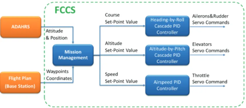
The “Mission Management” block of the FCCS supervises and controls the mission execution: the desired trajectory is assigned to the FCCS by means of a set of waypoints coordinates [32] and the “Mission Management” block

(37)

Flight Control Computer System | 25

computes the reference signals to be assigned to the control loops with the aim of performing the planned mission. As it can be observed in Figure 17, the heading-by-roll regulator acts on the ailerons and the rudder, the altitude-by-pitch computes the signals for the elevator, while the throttle command is computed by the airspeed controller.

Figure 17 - The interaction of the different sub-systems implemented on the FCCS.

In Figure 18 the block scheme of the altitude-by-pitch regulator is shown. The reference altitude is the height of the next waypoint to be reached. The current altitude is obtained by means of an EKF-based sensor fusion between the altitudes given by the on-board GPS and by the absolute pressure sensor of the ADAHRS board; the computed altitude is sent via CANAerospace protocol to the FCCS. The resulting error is processed by PIDAlt which provides the

reference signal to the inner loop, regulating the pitch angle.

(38)

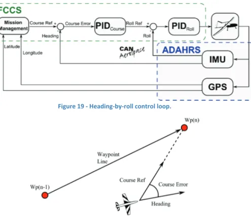
In Figure 19 the block scheme of the heading-by-roll control loop is shown. The course error is determined as it can be seen in Figure 20. The value of the desired course essentially depends on the coordinates of the next waypoint and the current coordinates of the aircraft (given by GPS); the measure of the heading is obtained from the ADAHRS. Obviously, this represents a simplification, because we are considering the heading as the direction in which the plane is pointing, without taking into account the effects of wind drift [26]. However, this problem is compensated by the FCCS navigation algorithm that continuously updates the Course Error. The resulting error is processed by the PIDCourse

regulator, which provides the reference signal to the inner loop, regulating the roll angle.

Figure 19 - Heading-by-roll control loop.

Figure 20 - Course error computation.

Finally, in Figure 21 the speed control block scheme is shown. The desired speed is related to the next waypoint, whereas the current speed is obtained

(39)

through a sensor fusion between the speed coming from GPS and the airspeed obtained by the differential pressure sensor connected to the Pitot tube.

Figure 21 – Speed control loop.

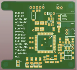
II.3.2 Hardware Design

The complete schematic of the FCCS subsystem is shown Appendix A. The main component is the dsPIC33FJ256GP710A, a microcontroller produced by Microchip [65]. Moreover, an EEPROM memory and a transceiver CAN are present. In Figure 22 the developed PCB is shown.

(40)

II.3.3 Operating modes

The operating modes of the FCCS determine the particular conditions in which the UAV operates, which results in a different iteration with the environment. Essentially, the operating modes necessary are two: the first is necessary for the tuning of the PIDs, and the second one is used to accomplish a given flight plan.

II.3.3.1 Assisted Mode

In assisted mode the aircraft does not follow any flight plan, but the reference values of the controlled variables (Roll, Pitch, Heading, Altitude and Speed) set by the user. This mode is particularly useful during calibration of the control loops or to verify the correct operations of them. Using the complete cascade control, it is possible to assign the reference to the variable on the outer loop (Heading and Altitude) Only. To assign the reference variables in the inner loop (Roll and Pitch) the outer loop should be opened, transforming the cascade control in a simple feedback control (in this configuration, yaw and altitude are not checked). For this reason two flags are inserted in the heading-by-roll and in the altitude-by-pitch control loops, TrackHold and AltitudeHold. These flags make it possible to set the reference of the outer loop, or inhibit it and give a reference value directly to the inner loop. As regards the speed control, being controlled by a simple feedback control, it always follows the reference set by the operator. This is summarized by Table 4 and Figure 23.

Flag →

Setpoints ↓ TrackHold True False AltitudeHold True False

RollAssisted Notused Used X X

TrackAssisted Used NotUsed X X

PitchAssisted X X Notused Used

AltitudeAssisted X X Used NotUsed

AirspeedAssisted X X X X

(41)

Figure 23 - Assisted Mode Flow chart

II.3.3.2 Navigation

This is the typical operating mode of the UAV, i.e. the navigation between waypoints. In this modality a waypoint is considered reached if the UAV is located within a given radius from it (typically chosen as 50m in this work). In Figure 24 the flow chart of this modality is shown.

(42)

Figure 24 - Navigation mode flow chart

II.3.4 Autotuning algorithm

The tuning procedures of the control algorithms of unmanned platforms represent one of the most time consuming phases, especially in the case of flying robots adopted in strongly not structured environments, like in volcanoes [11]. Usually a new mission needs to be preceded by a tuning procedure of the control loops, depending on weather and environmental conditions (pressure, temperature and so on). Propellers efficiency, wings lift and the power of a stroke engine depend on air density, which is strongly related to the weather conditions.

The implementation of automatic procedures represents an advantage that makes the development phase of an UAV easier and faster. Several papers deal with the automatic or self-tuning of control systems [34]. However, only a few

(43)

attempts are related to UAVs [28] [29] [30] [31]: this is mainly due to the risks connected to the tuning procedures of this kind of robotic platforms.

The relay feedback technique is widely adopted for the automatic tuning of PID controllers [27]. However, such algorithm is unsuitable for the automatic tuning of the control loops of an aircraft. Indeed, the first phase of this algorithm leads the system in a steady-state oscillation. It is clear how dangerous could be this condition for an aircraft. A different approach is based on Fuzzy rules, suggested by experience. The papers [28] and [29] are examples of this approach, where a self-adaptive fuzzy control is used to tune the PIDs of an UAV.

However, up to now the literature presents only works focused on the different methodologies to be adopted for the self or automatic tuning of UAVs. The step ahead is represented by the development of an hardware and software suite that makes the tuning phase safe, reliable and fast, independently of the control loops implemented on the on-board avionics [25].

The tuning algorithm analyses the step response of the control loop to be tuned and automatically implements a method based on Åström and Hägglund [27], where the PID parameters are chosen as a compromise between stability and speed, as summarized in Table 5.

Speed Stability Proportional Action increases Increases Reduces

Integral Action increases Reduces Increases

Derivative Action increases Increases Increases

Table 5 - Effect of the controller on speed and stability

Going into detail, a constant set-point is assigned to the control loop to be tuned and the response of the aircraft is analyzed to verify if the desired behavior is achieved. A set of constraints, assigned before the tuning procedure, must be satisfied: rise time, overshoot, steady state error and settling time (Figure 25). The values assigned to the constraints should be based on the specific aircraft model and, in general, on experience.

The algorithm, developed in Matlab-Simulink [68], communicates with the onboard avionics via CANAerospace protocol. A screenshot of the GUI implemented for executing and monitoring the tuning procedure is shown in Figure 27: in particular, the form dedicated to the automatic tuning is represented. This form allows the operator to assign the desired constraints (“Specifications” section), to start the tuning procedure (“Auto Tuning” section),

(44)

to analyze in real-time the response of the control loops (“Step Response” section) and to view the computed parameters (“Dynamic Features” section).

Figure 25 - Generic step response

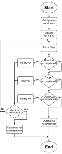
The tuning procedure, automatically executed by the implemented algorithm and started by acting on the “Auto Tuning” section of the GUI, is shown in Figure 26 and summarized below:

• The constraints must be introduced in the “Specifications” section of the developed HMI.

• An initial set of the PID parameters is assigned and sent via CANAerospace to the control loops of the FCCS.

• A step signal is assigned as input reference for the autopilot.

• The dynamic response of the system is analyzed and is compared with the assigned constraints.

If the response is not satisfactory, the PIDs gains are modified according to the following classical rules [27]:

• The proportional action is correlated to the speed and, then, to the rise time;

• The derivative action is correlated with the overshoot; • The integral action acts on the steady state error.

(45)

This procedure is iterated until the constraints are not satisfied or a specified number of iterations is reached.

(46)

Figure 27 - The developed GUI for the autotuning procedure

II.3.5 HIL Architecture

Hardware in the Loop architectures have been adopted by several projects to develop and test different aeronautical components [33] [35] [36].

To reduce time, costs and risks related to the trials on a real aircraft, an HIL architecture has been used to test and verify the developed architecture: the real aircraft has been substituted with a simulated virtual model closed in a HIL architecture with the real controller.

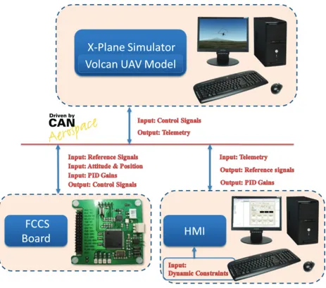
The used HIL architecture is similar to the one adopted in [32] to develop the VOLCAN project. In this architecture the VOLCAN has been replaced by the X-Plane Simulator by Laminar Research [53], connected both to the FCCS and the GUI via CANAerospace. In Figure 28 the adopted architecture is shown; the block named “FCCS” represents the real electronic board. Telemetry data, concerning plane pose, are sent from the simulator through CANbus to the FCCS board by using the CANaerospace protocol. Once attitude and position of the aircraft are known, the control algorithms implemented on the FCCS board compute the signals for the servo commands that are sent back to the simulator to actuate the mobile parts of the plane.

(47)

The GUI, presented in II.3.4, is closed in the loop to execute the automatic tuning procedure, sending the reference signals to the FCCS and capturing and recording the telemetry data sent by the simulator.

In the next paragraphs, several experimental results are presented. In particular, in the first part the procedure and the results related to the automating tuning of the “heading-by-roll” control loops (Figure 19) are discussed. The first step regards the tuning of the inner (and faster) variable, the roll (II.3.5.1). Once the roll loop has been tuned, the procedure to tune the outer loop (heading, with a slower dynamic) is automatically executed (II.3.5.2).

To validate the results of the automatic tuning algorithm, the computed parameters have been used during the execution of a complete flight mission in absence of wind (II.3.5.3) and in windy conditions (II.3.5.4).

(48)

II.3.5.1 Automatic tuning of the roll control loop

To tune the roll control loop, the outer loop (heading control) is deactivated and the reference signal is directly assigned to the inner control loop.

To execute this procedure, the aircraft has been placed at an altitude of 200m ASL, with a ground speed of 90 Km/h. The reference roll signal used to evaluate the step response has been set to ±30°: the procedure is considered as successfully completed when the constraints are satisfied both on the positive (+30°) and the negative (-30°) roll steps.

The constraints to be satisfied, assigned at the beginning of the procedure, are reported in the first row of Table 6; the second row reports the values reached at the end of the tuning procedure.

The initial values of the PID gains are shown in the first row of Table 7, while the computed parameters are reported in the last row.

Parameters Rise time _[s] Settling time _[s] Overshoot [DEG] Overshoot _[%] _[DEG]SSE Imposed 1 1 0.3 1 0.3

Achieved 0.82 0.82 0.17 0.58 0.21

Table 6- Constraints and results of roll loop tuning.

Gains Kp Kd Ki Starting values 1.5 0 0

Final values 2.4 0 0

Table 7 - Roll PID gains.

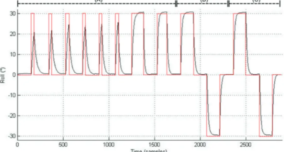
Figure 29 shows the time evolution of the roll angle, measured during the tuning procedure. As it can be observed, the responses of the first eighth steps are incomplete (A), because the constraint related to the rise time on the positive edge is not satisfied. In fact, when the reference signal is not reached in the assigned rise time, the algorithm stops the step under execution; then, the KP gain is modified and another step is executed.

At the ninth step (B), the constraints are satisfied on the rising edge of the +30° imposed roll; but they are not satisfied on the negative step.

(49)

Finally, at the tenth attempt (C), the algorithm executes positive and negative steps and verifies that the imposed constraints are achieved (Table 6), by acting only on proportional action (Table 7).

Figure 29 - Roll control loop auto-tuning procedure

II.3.5.2 Automatic tuning of the heading control loop

Once the roll loop has been tuned, the outer loop (heading) is reactivated while the PID gains of the inner loop (roll) are those achieved in the previous roll loop tuning. In this case, the reference amplitude, used to evaluate the step response, has been imposed to ±45°. Constraints and results are summarized in Table 8, while the achieved PID gains are shown in Table 9.

Parameters Rise time _[s] Settling _{time [s]} Overshoot _[DEG] Overshoot [%] SSE _[DEG] Imposed 6 6 2 4.44 2

Achieved 4.2 4.26 0.44 1 1.25

(50)

Gains Kp Kd Ki Startingvalues 0.8 1 0

Increments 0.1 0.1 0.01

Finalvalues 1 1.2 0.01

Table 9 - Heading PID gains

In Figure 30 the result of the heading control loop automatic tuning procedure is shown. Likewise to the roll tuning procedure, the first two steps (A) are partial, because the rise time constraint is not satisfied on the positive edge; then, the constraints are satisfied for the positive edge but not on the negative edge (B). Finally, the assigned specifications are satisfied both on the positive and the negative edges (C).

In order to tune the remaining control loops (pitch, altitude and speed) automatic tuning procedure have been executed and the algorithm has always found suitable PID gains satisfying the imposed constraints.

(51)

II.3.5.3 Parameters validation: mission execution without wind

The same procedure used for the “heading-by-roll” control loops has been adopted for the automatic tuning of the “altitude-by-pitch” and “speed” control loops.

Then, a mission has been executed in the HIL architecture to validate the obtained parameters. In Figure 31 the mission is represented: the red circles are the assigned WPs while the purple line represents the executed trajectory. Table 10 summarizes the assigned WPs and the altitude and speed assigned for each one.

Waypoint Latitude

[Deg] Longitude [Deg] Altitude [m] [km/h]Speed WP1 37.4728737 15.0714064 200 80

WP2 37.4591484 15.0772877 500 110

WP3 37.4603195 15.0517006 300 90

Table 10 - Waypoint assigned for parameters validation

Figure 31- The mission executed after the automatic tuning procedure

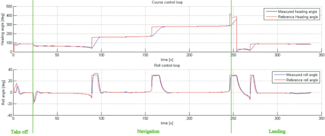
Figure 32 allows to observe the behaviors of the two control loops involved in the “heading-by-roll” regulation during the mission. The picture shows the time evolution during the take-off, navigation and landing phases.

(52)

Figure 32 - The time evolution of the heading-by-roll control loops

In Figure 33 the time evolutions of the control loops involved in the “altitude-by-pitch” regulation is shown.

As it can be observed by analyzing Figure 31, Figure 32 and Figure 33, the behavior of the tuned loops is fine and allows to execute the flight plan in a satisfactory way.

(53)

II.3.5.4 Parameters validation: mission execution in windy conditions

To validate the robustness of the control architecture with the parameters computed by the automatic tuning algorithm, the same mission assigned in the previous section has been executed in windy conditions, introducing in the simulator a wind of 20 km/h and with the direction shown in Figure 34. Such a wind condition is remarkable taking into account the aircraft under test.

Figure 34- The mission executed in windy conditions. The red arrow indicates the wind direction.

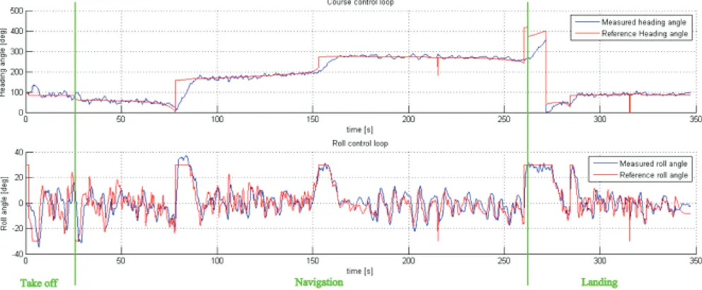
Figure 35 allows to observe the behaviors of the two control loops involved in the “heading-by-roll” regulation during the mission. The picture shows the time evolution during the take-off, navigation and landing phases.

In Figure 36 the time evolutions of the control loops involved in the “altitude-by-pitch” regulation is reported.

As it can be observed by analyzing Figure 35 and Figure 36, the response of the inner loops (roll and pitch) allows to obtain a good behavior of the outer loops (heading and altitude). This permits the aircraft to reach successfully the assigned waypoints, even if the trajectory is disturbed.

(54)

Figure 35 - The time evolution of the heading-by-roll control loops in windy conditions.

(55)

Servo Actuators Control System | 43

II.4 Servo Actuators Control System

This subsystem manages the engine and the actuators (up to seven) connected to the mobile parts of the Volcan UAV. It also allows switching from the UAV mode to the Pilot In Command (PIC) mode, in order to execute takeoff and landing operations or also to bypass instantaneously the FCCS in case of failures. Therefore, in UAV mode the reference signals come from the FCCS, whereas in PIC mode they come from the RC receiver. The core of the SACS is the microcontroller PIC18F4580 by Microchip [65]. Moreover, a transceiver CAN and an array of digital isolators, in order to isolate the ground of the servos (generally noisy) with the ground of the microcontroller, are mounted. PCB of the SACS is shown in the following figure, whereas the schematic is reported in Appendix A.

(56)

II.5 UDP2CAN

This subsystem acts as a bridge between the CANAerospace bus and a wireless link. This is because it is necessary for the operator to supervise and monitor the drone by means of a ground station. Obviously, a wireless link does not have the same robustness of a wired link. However, considering that the ground station receives only telemetry data and it sends asynchronous commands with ACKs (the NSH frames), it's clear as this type of connection represents an appropriate solution.

Going into details, an UDP2CAN bridge has been realized, i.e. a device that converts CAN frames coming from the drone control system in UDP frames suitable for a commercial WiFi link.

As regards the hardware, this subsystem has the same microcontroller of the FCCS, the dsPIC33FJ256GP710A, in addition to a transceiver CAN (MAX3051) and the ENC28J60, an Ethernet controller produced by Microchip [65]. PCB of the UDP2CAN is shown in the following figure, whereas its schematic is reported in Appendix A.

(57)

Air Data and Attitude Heading Reference System | 45

II.6 Air Data and Attitude Heading Reference System

The last subsystem of the whole control architecture is represented by the ADAHRS. In reality, for reasons of convenience, this subsystem is split into two boards:

• A sensors board, which manages GPS, pressure sensors and temperature sensor.

• An Inertial measurement unit, that gives information about attitude and heading. To this board, considering its complexity, the section II.7 is dedicated.

II.6.1 Sensors Board

The dsPIC33FJ256GP710A onboard manages the following sensors: • A classical GPS with RS232 interface.

• The STTS75 Digital temperature sensor.

• The absolute pressure sensor HSCMAND015PA2A3 by Honeywell [66], used as barometer in order to obtain information about altitude. • The differential pressure sensor HSCMRRN100MD2A3 by

Honeywell [66], used as Pitot tube in order to obtain information about airspeed.

PCB of the sensors board are shown in the following figures. Its schematic is shown in Appendix A

(58)

II.7 IMU board

The aim of this board is to provide the Euler angles of the aircraft. To make this possible, a set of inertial sensors are needed. Such a set of sensors, together with a 32bit ARM microcontroller, are present in the INEMO®_{-M1, produced by}

ST-Microelectronics [37]. Going into details, the key features of this device are the following:

• STM32F103REY6: WLCSP package, high-density performance line ARM®-based 32-bit MCU

• LSM303DLHC: 6-axis digital e-compass module, ±2g, ±4g, ±8g, ±16g linear acceleration programmable full scale, from ±1.3 gauss to ±8.1 gauss, I2_{C digital output}

• L3GD20: 3-axis digital gyroscope (roll, pitch, yaw), 16-bit data output, ±250°/s, ±500°/s, ±2000°/s selectable full scale

• LDS3985M33R: ultra-low drop, low-noise BiCMOS 300 mA onboard voltage regulator.

• Flexible interfaces: CAN, USART, SPI and I2_{C serial interfaces; full-speed}

USB 2.0

• Up to 8 ADC channels for external analog inputs • Compact design: 13 x 13 x 2 mm

Figure 40 - INEMO®_-M1

II.7.1 Hardware development

In order to interface the INEMO®_{-M1 with the other subsystems, some}

improvements have been added. In particular, a transceiver CAN and an SWD connector (to program the microcontroller) were inserted. In the following figure, the board is shown. The schematic is in Appendix A.

(59)

IMU board | 47

Figure 41 - INEMO®_{-M1 Board}

II.7.2 Firmware development

The IMU firmware development has represented one of the most complex phases in the design of the Volcan control system. The reason is that to develop a reliable system that calculates the RPY angles from a set of inertial sensors requires a very long phase of test and optimization. In the next paragraphs the various development and optimization steps are described.

II.7.2.1 CANAerospace implementation

The first step in the IMU development is represented by the implementation of the CANAerospace protocol. The CANAerospace directives impose only the most important frame structures, such as the frames for the RPY angles. There is therefore the possibility to insert several user defined frames, in order to make possible the management and the personalization of such a system. A complete documentation of the CANAerospace protocol implemented is reported in Appendix B.

II.7.2.2 Extended Kalman Filter implementation

The classical Kalman filter [38] [39] is an optimal observer under the hypotheses that the system is linear and that both the process and the measurement noises are Gaussian and additive. The Kalman Filter equations are summarized in Table 11

(60)

Initial estimates for and Time Update (“Predict”) Project the state ahead = + Project the error covariance ahead = +

Measurement Update (“Correct”)

Compute the Kalman gain = ( + ) Update estimate with measurement zk = + ( − )

Update the error covariance = ( − )

Table 11 - Kalman Filter Equations

Unfortunately, in this case of study the hypothesis of linearity is not satisfied. However, under the assumption that the process and the measurement noises are Gaussian and additive, it is possible to implement an Extented Kalman Filter (EKF) algorithm [40] [41]. With respect to a conventional Kalman filter, the EKF is its linearization around the current estimate. Considering a given process with the following equations:

= ( , , )

= ( , )

Where xk represents the state variables, zk the measurements and f, h non-linear functions. The following Jacobians represent the non-linearization of the system around the current estimate:

[ , ] = [ ] [ ]( , , 0) [ , ]= [ ] [ ]( , , 0) [ , ]= ℎ[ ] [ ]( , 0) [ , ]= ℎ[ ] [ ]( , 0)