Data mining techniques on volcano monitoring

U

NIVERSITÀ DEGLI

S

TUDI DI

C

ATANIA

F

S

MM.

FF.

NN.

D

M

I

DOTTORATO DI RICERCA IN INFORMATICA - XXVCICLO

Marco Antonio Aliotta

DATA MINING TECHNIQUES ON VOLCANO MONITORING

ANNO ACCADEMICO 2011-2012

Tutor:

Dott.Ing. P. Montalto (INGV-OE) Dott. Alfredo Pulvirenti (UNICT-DMI)

Preface

The aim of this thesis is the study of data mining process able to discover implicit information from huge amount of data. In particular, indexing of datasets is studied to speed the efficiency of search algorithm. All of the presented techniques are applied in geophysical research field where the huge amount of data hide implicit information related to volcanic processes and their evolution over time. Data mining techniques, reported in details in the next chapters, are implemented with the aim of recurrent patterns analysis from heterogeneous data.

This thesis is organized as follows. Chapter 1 introduces the problem of searching in a metric space, showing the key applications (from text retrieval to computational biology and so on) and the basic concepts (e.g. metric distance function). The current solutions, together with a model for standardization, are presented in Chapter 2. A novel indexing structure, the K-Pole Tree, that uses a dynamic number of pivots to partition a metric space, is presented in Chapter 3, after a taxonomy of the state-of-the-art indexing algorithm. Experimental effectiveness of K-Pole Tree is compared to other efficient algorithms in Chapter 4, where proximity queries results are showed. In Chapter 5 a basic review of pattern recognition techniques is reported. In particular, DBSCAN Algorithm and SVM (Support Vector Machines) are discussed. Finally, Chapter 6 shows some geophysical applications where data mining techniques are applied for volcano data analysis and surveillance purpose. In particular, an application for clustering infrasound signals and another to index an thermal image database are presented.

Acknowledgments

“First I would like to thank my scientific colleagues for their fundamental cooperation:

Dr. Andrea Cannata, Dr. Carmelo Cassisi and Dr. Ing. Michele Prestifilippo, loyal friends as

well as colleagues. Without their help this thesis would not have been possible. Many thanks

to my tutors Prof. Alfredo Pulvirenti and Dr. Ing. Placido Montalto. A particular mention to

Placido,

whose friendship since my childhood has supported my personal growth.

In addition, I would like to express my sincere gratitude to Prof. Alfredo Ferro and Dr.

Domenico Patanè, Director of “INGV – Osservatorio Etneo” for their constant guidance

and encouragement.

In the end, I wish to warmly thank my family for their support and the great help they have

given me. Last, but not least, a special thought goes to my girlfriend Elisabetta who has

always encouraged me to accomplish this work”.

1. Indexing and searching in metric space ... 1

1.1 Key Applications ... 3

1.1.1 Query by Content in Structured Database ... 3

1.1.2 Query by content on multimedia objects ... 4

1.1.3 Text Retrieval ... 5

1.1.4 Computational biology ... 6

1.1.5 Pattern Recognition and Functions Approximation ... 6

1.1.6 Audio and Video Compression ... 7

1.2 Basic Concepts ... 7

1.3 Proximity Query ... 9

1.4 Vector Spaces ... 11

2. Overview of Current Solutions ... 13

2.1 Discrete Distance Functions ... 13

2.2 Continue Distance Functions ... 14

2.3 Other techniques ... 15

2.4 Approximation and probabilistic algorithms ... 16

2.5 Summary Table ... 16

2.6 A Model for Standardization ... 18

2.7 Indexes and Partitions ... 19

2.8 Efficiency measures ... 20

2.9 Location of a partition ... 21

2.10 Intrinsic Dimension ... 22

3. Taxonomy of Searching Algorithms: K-Pole as a case of study ... 25

3.1 The Relation of Equivalence of Pivots ... 26

3.2 Selecting Pivots ... 27

3.3 Search Algorithms ... 28

3.4 Comparisons between existing Data Structures ... 30

3.5 Considerations and Open Problems ... 31

3.6 The Antipole Tree ... 32

3.7 Calculation of Diameter (Antipole) ... 35

3.8 How Antipole Tree works ... 35

3.9 Antipole Tree in generic metric spaces ... 36

3.10 Construction of the Tree ... 37

3.12 The calculation of the k centers of a set (K-Pole) ... 38

3.13 Gonzalez algorithm ... 40

3.13.1 Possible optimizations of Gonzalez Algorithm ... 41

3.14 The Data Structure ... 42

3.14.1 From Binary Tree to k-ary Tree ... 42

3.14.2 Inner nodes and clusters ... 44

3.14.3 The construction of the Tree ... 45

3.15 Dynamic k cardinality evaluation ... 47

3.16 The Range Search Algorithm ... 48

3.16.1 The procedure RANGE_SEARCH ... 49

3.16.2 The procedure VISIT_CLUSTER ... 50

3.17 The k-Nearest Neighbor Search algorithm ... 52

3.17.1 The procedure KNN_SEARCH ... 52

3.17.2 The procedure KNN_VISIT ... 54

3.17.3 The procedure KNN_VISIT_CLUSTER... 55

3.17.4 The procedure CHECK_ORDER ... 55

3.18 Caching Distance Calculations ... 56

4. Experimental Results (in Range Search and KNN Search) ... 58

4.1 Static K-Pole VS Dynamic K-Pole ... 58

4.2 K-Pole VS Other Index Structures... 59

4.3 Pivots decreasing rate ... 61

5. Pattern recognition analysis methods ... 63

5.1 Clustering: an overview ... 64

5.1.1 Hierarchical vs. partitional algorithms ... 66

5.1.2 Cluster assessment ... 68

5.1.3 Squared error clustering and k-means algorithm ... 69

5.1.4 Clustering algorithm based on DBSCAN ... 72

5.1.5 Features classification using SVM ... 73

5.2 Model selection ... 75

6. Data Mining in Geophysics ... 79

6.1.1 Clustering and classification of infrasonic events at Mount Etna using pattern recognition techniques ... 79

6.1.2 Infrasound features at Mt. Etna ... 80

6.1.3 Data Acquisition and Event Detection ... 82

6.1.5 Semblance Algorithm ... 85

6.1.6 Learning phase ... 86

6.1.7 Testing phase and final system ... 89

6.2 Data mining in image processing: Stromboli as a case of study ... 93

6.2.1 Morphological image analysis ... 93

6.2.2 Thermal Surveillance at Stromboli volcano ... 96

6.2.3 Mapping Explosions into a Metric Space ... 97

1.

Indexing and searching in metric space

The problem of the search for elements of a set being close respect to a query element, according to a similarity criterion, has a wide range of applications in computer science, from pattern recognition to information retrieval, both textual and multimedial.

The case we want to focus on is the one where the similarity criterion defines a Metric Space, rather than dwelling on spatial vectors. For this purpose, a large number of solution for different areas were proposed, in many cases developed without cross – knowledge.

Because of this, the same ideas have been reinvented several times and have been given different presentations for the same approach. We now present a unified view of all the proposals to build Metric Spaces, to include their organization through a common model. Many approaches appear to be variations of a few basic concepts. We will organize this work into a taxonomy that allows us to separate the new algorithms from combinations of concepts that were not disclosed earlier because of the lack of communication between the different communities.

Some of the new techniques, created as combinations of the above have proven very competitive

We present experiments that confirm our results and compare them to existing approaches, in order to determine the optimal solution for our problem. At the end of this chapter we show some recommendations for those who engage with this problem and open questions for future developers.

Research is a fundamental problem of computer science, present in virtually all of its applications. In some of these, exposed search problems are very simple, while in others, more complex, it requires a more sophisticated form of search.

Search operation is typically performed on particular data structures, e.g. alphabetic or numeric information, which are scanned exactly. In this case, given a query, the set of strings exactly equal to the query itself is returned. Traditional databases are built around the concept of exact search: they are divided into records, each with a well-defined and comparable key. A query made to the database will return all records whose keys match the query.

There are more sophisticated types of research, such as range queries on numeric key or the search for a prefix of alphabet keys, which are based on the concept that the keys may be identical or not, or there is a linear ordering among the total keys. Even in recent

times, when in databases was made possible to storing new data types like images, research has yet been performed on a predetermined number of numeric or alphabetic keys.

With the evolution of information and communication technologies, collections of unstructured information are emerged. Not only different types of data as simple text, images, audio and video can they be asked; also to structure the information in records and keys is no longer possible. Such structuring is very a difficult task (both from human and computational point of view) and narrows in advance the types of queries that can be placed after. Even when a classical structure is possible, new applications such as data mining require access to the database through any field, not just those marked as key. Therefore, you need new models for searching collections of unstructured data.

The scenarios just discussed require more general search algorithms and models than those classically used for simple data. A unifying concept is that search of similarity or proximity, i.e. the search for database elements that are similar or close to a given element (query). The similarity is modeled with a distance function that satisfies the triangular inequality, and the set of objects is called a Metric Space. Since the problem has appeared in different areas, the solutions in their turn have appeared in many fields, also disconnected from each other, as statistics, artificial intelligence, databases, computational biology, pattern recognition and data mining, and others. With solutions from several fields, it is not surprising that the same solutions have been reinvented many times, as an obvious combination of solutions that had not yet been disclosed, and that had not been against analytical or experimental comparisons. Above all, it has never been attempted to unify all of these solutions.

In many applications, the general problem is traversed from metric spaces in a vector space (the objects are represented as k-dimensional points with some interpretations of geometric similarity). It because the concept of similarity search appeared in first place in the spaces vector. This is a natural extension of the problem of finding the point closer to a plan. In this model there are optimal algorithms (on the size of the database) in both the average case that in the worst case [10] for the search of the nearest point. Search algorithms for vector spaces are called space access methods (SAM). Among the most popular, we include the kd-trees [8, 9], R-trees [36] and the most recent Xtrees [11] (see also [57, 35] for an overview). Unfortunately, existing algorithms are strongly affected by the size of the vector space: search algorithms depend exponentially on the

size of the space (this is called “curse of dimensionality”). In practical terms, we consider that the problem becomes intractable when it exceeds the 20 dimensions. For this reason, many authors have proposed the use of a distance based on indexing techniques, which uses only the distance between the points and avoids reference to the coordinates, in order to avoid the curse of dimensionality.

This may be particularly effective when a set with an intrinsically low dimension is “embedded” within an artificial more dimensional set (e.g. a plan within a three-dimensional set). Therefore, generic metric spaces can be used, not only when the problem is not structured in coordinates, but also when the number of these coordinates is very high.

With respect to generic metric spaces, the problem has been addressed by several points of view. The objective in general is to build a data structure (or index) to reduce the number of calculations of distances at the time of query execution, since it is assumed that the distance is expensive to compute.

Some important progresses were made, especially in database communities, where a certain number of indexes and data structures based on distances were developed and studied from different perspectives.

1.1 Key Applications

In the following sections, we present some applications in which the concept of finding proximity appears. Since we have not yet submitted a formal model, we will not try to explain the connections between applications, but will resume the treatment of this in the next section.

1.1.1 Query by Content in Structured Database

In general, a given query to the database presents a fragment of a record information, and we need to find the entire record. In classical approach, the fragment presented is fixed (the key). In addition, the search for a key that is incomplete or incorrect is not allowed. On the other hand, in the most general approach required nowadays, the concept of search with a key is generalized to the search from an arbitrary subset of records, which present or not errors.

This kind of research has earned a great variety of names, e.g. range query, query by content or proximity searching. It is used in data mining (where the interesting parts of the records cannot be predetermined), when the information is not accurate, when we look for a certain range of values, when the search key may contain errors (e.g. a word that contains misspelling), etc.. A general solution to the problem of range queries from any field of a record is the Grid File [46]. The domain of a database is considered as a hyper-rectangle of size k (one for each field in the record), where each size has a sort of solidarity to the domain of the field (numeric or alphabetically). Each record in the database is considered as a point within the hyper-rectangle. A query specifies a sub-rectangle (e.g. a interval along each dimension), and returns all the points in the latter. This does not address the problem of searching of not traditional data types, or mistakes that cannot be recovered with a range query. However, it converts the problem of original research to the problem of obtain, in a given space, all points “close” to a given query point. Grid Files essentially consist of an organization technique of the hard disk in order to obtain effective range queries in secondary memory.

1.1.2 Query by content on multimedia objects

New data types like images, fingerprints, audio and video (called “multimedia” data types) cannot be questioned appropriately using the classic way. Not only they cannot be ordered, but they cannot be compared for equality. Applications will never have interest in finding an audio segment that is equal to another given segment. Nonetheless, the probability that two different images are equal “pixel by pixel” is negligible unless they are digital copies of the same source. In multimedia applications, all queries require objects similar to the one given. Some important applications are recognition of well-defined biometric features (face, fingerprint, voice), and multimedia databases in general [1].

An example is a collection of images. Interesting queries could be something like: “find a picture of a lion with the savannah in the background”. If the collection is labeled, and each label contains a full description of what the image contains, then our query example can be solved with a classical scheme. Unfortunately, this classification cannot be performed automatically with the image processing technology available today. The recognition of an object in real-world scenes is still in an immature state to perform tasks of this complexity. Moreover, we cannot predict in advance all queries that could

be used to label images for all possible types of requests. An alternative to the automatic classification consists in considering the query as an image of example, so that the system looks for all the images similar to the query. This can be constructed within a more complex system of feedback where the user approves or rejects the found image, and a new query is submitted with the approved images. It is also possible that the query is only a part of an image and the system must recover the entire image.

These approaches are based on the definition of a similarity function between objects. These functions are provided by an expert, but they pose no assumption about the type of query can be absolved. In many cases, the distance is obtained through a set of k "features" that are extracted from the object (e.g. in an image, a useful feature is the average color). Then, each object is represented by its k characteristics (an object becomes a point in a k-dimensional space) and we are once again in the case of a range query on a vector space. There is a growing community of scientists deeply involved with the development of such similarity measures [20, 12, 13].

1.1.3 Text Retrieval

Although it is not properly considered a multimedia data type, the finding of unstructured text poses problems similar to the finding of multimedia data. This is because text documents are generally unstructured, and this does not allow you to easily find the desired information. Textual documents can be interrogated to find strings that are present or not, but in many cases it is asked to find semantic concepts of interest. For example, an ideal scenario would allow the search on a text dictionary for a concept such as “free from obligations”, finding the word “ransom”. Such research problem cannot be properly established with the classic tools. A large number of researchers have worked on this problem for a long time [48, 34, 7]. A certain amount of similarity measures was revealed. The problem is mainly solved finding documents similar to a given query. You can even submit a document as query, so that the system finds documents similar to it.

Some approaches which make use of similarity are based on the mapping of a document into a vector of real values, in so that each dimension is a dictionary word and the importance of word in the document (prepared by some formula) is the coordinate of the document in this dimension. In this space functions similarity are defined. Note however that the number of dimensions of the space is really high (we talk of thousands

of dimensions, one for each word). Another problem related to the discovery of text is typing. Since more and more text databases with low quality control appear (just think about the World Wide Web to get an idea), and typing mistakes or those of using an OCR (optical character recognition) are commonplace both in the text that in the query, we have that document in which appears a word that contains a spelling error is no longer retrievable from a misspelled queries. There are patterns of similarity between words (changes in distance editing [49]), which work very well with the presence of such errors. In this case, given a word, you want to find all the words like it. Another application is related to spell checking, where we try (correct) variations of a mistyped word.

1.1.4 Computational biology

DNA and protein sequences are the basic objects of study in molecular biology. Since they can be modeled as strings, we refer to the problem of finding a given (sub) sequence of characters within a string. However, the fact that an exact overlap occurs is unlikely, and computational biologists are more interested in discovery of parts of longer sequences that are similar to the (small) given sequences. The reason that research is not exact is due to small difference chains that describe genetic creatures of the same species or similar. The similarity measure used is linked to the probability of mutations [56, 49]. Other problems are related to the construction of phylogenetic trees (a tree which graphically shows the evolutionary path of one or more species), the search for pattern of which only certain properties are known, and more.

1.1.5 Pattern Recognition and Functions Approximation

A simplified definition of pattern recognition is the construction of a approximator of functions. In this formulation of the problem we have a certain finite number of data samples, and each of them is labeled as belonging to a certain class. When a new sample of data is given, the system is required to label the sample with one of the labels of the known data. In other words, the classifier can be imagined as a function defined from a space of objects (samples of data) and to values into a set of labels. In this sense, all classifiers can be approximators of considered functions.

If the objects are m-dimensional vectors of real numbers, then a choice are the natural neural networks and fuzzy approximators of functions. Another popular universal approximator of functions, the k-nearest neighbor classifier, finds the k nearest objects to the not labeled sample, and assigns it the "majority" label of the k nearest objects. In contrast to neural networks and fuzzy classifiers, k-nearest neighbor technique has no training costs, but it has linear complexity if it does not use any indexing algorithm [31]. Other applications of the k-nearest neighbor classifier are estimated density [30] and learning "reinforcement" [52]. In general, any problem where it is desired to infer a function based on a finite set of samples of data represents a potential application.

1.1.6 Audio and Video Compression

The audio and video transmission over a narrow band channel is a key problem, for example in the audio / video conferencing based on the Internet. A frame (a static image in a video, or audio fragment) can be thought as formed by a certain amount of (possibly overlapping) sub-frames (16 x 16 sub-images in a video, for example). In a really brief description, the problem can be completely solved by sending the first frame, and for the subsequent frames sending only the sub-frame that has a significant difference with the earlier sub-frame. This description includes the MPEG standard. The algorithms, in fact, use an under-frame buffer. Each time that a frame is going to be sent, it is searched (with a threshold of tolerance) in the sub-frame buffer and only if that fails then the whole sub-frame is added to the buffer. If the sub-frame is found then it is shipped only the index of similar frames found. This implies, of course, that a fast search algorithm of similarity should be embedded in the server in order to maintain a minimum rate of frames per second.

1.2 Basic Concepts

All the applications presented in the previous section share a common model, which basically consists in finding the nearest objects in according to a suitable similarity function, within a finite set of elements. In this section, we present the formal model that includes all cases discussed above.

We now introduce the basic notation for the problem of the discharge of proximity queries. The set X will denote the set of right or valid objects. A finite subset of them, U of cardinality n = | U |, is the set of objects where the search is performed. U will be called the dictionary, database, or simply our collection of objects or elements. The function d: X X  R denotes the distance measure between objects (in particular the shorter is the distance, the closer or more similar will be the objects). The distance functions have the following properties:

(p1) x, y X, d (x, y)  0 positivity (p2) x, y X, d (x, y) = d (y, x) symmetry (p3) x X, d (x, x) = 0 reflexivity and in many cases

(p4) x, y X, x y  d (x, y) > 0 strict positiveness

The properties of similarity listed above provide only a consistent definition of the function, and cannot be used to save distance computations in a proximity query. If d is really a distance, that is, if it satisfies

(p5) x, y, z X, d (x, y) d (x, z) + d (z, y) triangle inequality then the pair (X, d) is called a metric space.

If the distance function does not satisfy the property of strict positiveness (p4) then the space is called metric space. Although for simplicity we do not consider pseudo-metric spaces in this work, all the presented techniques are easily adaptable to simply identify all the objects with zero distance as one single object. This process works because if (p5) is valid, it is easy to prove that

d (x, y) = 0 z, d (x, z) = d (y, z).

In some cases we can have an almost – metric space, where the symmetry property is not valid (p2). For example, if the objects are corners of a city and the distance corresponds to the distance a car must travel to move from one corner to another, then the existence of one-way streets makes the distance asymmetric. There are techniques to

derive the new symmetric distance function from an asymmetric one, as d1(x, y) = d (x, y) + d (y, x).

However, in order to limit the search range of a query when we use a symmetric function, we need a specific knowledge of the domain.

Finally, we relax the triangle inequality (p5) to d(x, y) d(x, z) + d(z, y) + , and after some scaling we can search within this space using the same algorithms designed for metric spaces. If the distance is symmetric, then for consistency should be  = .

1.3 Proximity Query

There are mainly three types of queries of a certain interest in the metric spaces: (a) Range Query (or proximity query)

Returns all elements that lie within a certain distance r from q, that is {u  U / d (q, u)  r}. We denote this query as (q, r)d.

(b) Nearest Neighbor Queries

It finds items nearest to q in U, that is {u  U / v U, d (q, u)  d (q, v)}. In some cases we just find a single item (in continuous spaces still there is normally only one element that satisfies the query).

We may also impose a maximum distance r* (tolerance threshold), such that if the closest element is at a distance greater than r* from the query, then it will not return any items.

(c) k-Nearest Neighbor Query

It finds the k closest elements to q in U, which determines a set A U such that:

| A | = k  u  A, v  U – A, d (q, u)  d (q, v). Note that in the case of equal elements, any set of k elements that satisfy the condition will be acceptable.

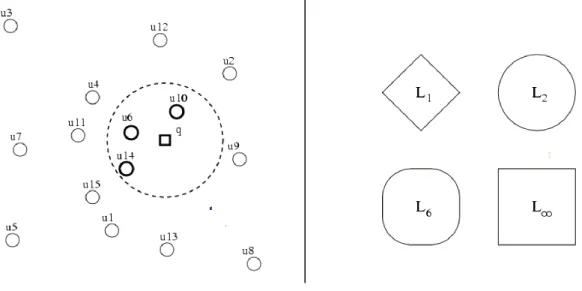
The most basic type of query is of the type (a). The left part of Figure 1 shows a query on a set of points that we use as an example. For simplicity we will use R2 as metric space. A proximity query will be so close to a pair (q, r)d, with q element (possibly) not

belonging to X and a real number r that indicates the radius (or tolerance) of the query. The set {u  U / d (q, u)  r} will be called the result of the proximity query. The query

is specified as a query "d-type" because for different distance functions there will be different query results (e.g. using the Euclidean distance we will have a different result from what we would get using the Manhattan distance, etc.).

The other two types of queries are usually fixed by using a variant of range queries. For example, the query type (b) is usually solved as a range query where the radius is initially placed as infinite, and is decreased at a distance less and less as elements closer to the query are found.

This is usually coupled to a heuristic trying to get items that are close to the query as soon as possible (the problem is increasingly easy for small radii). The queries of type (c) are normally resolved as a variant of type (b), where at each instant the k-nearest elements are maintained and the current radius is the distance between the query and the farther object from these k elements (given that most distant of these elements become free of interest).

Another widely used algorithm for query of type (b) and (c) based on those of type (a) is to search with fixed radius r = 2i, starting with i = 0 and incrementing until the desired number of elements (or more) "falls" in the search radius r = 2i. After that, the radius is redefined from r = 2i-1 to r = 2i, until the exact number of elements is included.

The total CPU time for calculating a query can be divided into

T = # distance calculations  d( ) complexity + extra CPU time and we want to minimize T.

In many applications, however, d() computation is so expensive that the extra CPU time can be neglected. This is the model that will be used in this thesis, and therefore the number of calculated distances will measure the complexity of the algorithms. We also take into account a certain amount of linear CPU (but reasonable) work, as soon as the number of distance calculations remains low. However, we set to some extent also the attention to the so-called extra CPU time.

It is clear that all the query types mentioned above may be solved examining the entire dictionary U. In fact, if we are not allowed to perform a preprocessing on the data, e.g. building the index data structure, then exhaustive investigation remains the only way forward. An Indexing Algorithm is an off-line procedure that builds in advance a data

structure (or index), designed to save distance computations during the execution of proximity queries. This data structure can be expensive to build, but the cost spent in the construction process will be amortized saving distance computations on many queries posed to the database. The intention is, therefore, to design efficient indexing algorithms in order to reduce the number of distance calculations. All these structures are working on the basis of discarding elements using the triangle inequality (the only property that actually saves distance computations).

1.4 Vector Spaces

If the elements of the metric space (X, d) are t-uples of real numbers (actually t-uples of any field) then the pair is called a finite-dimensional space vector, or more briefly a vector space.

A k-dimensional vector space is a particular metric space where objects are identified with k real-valued coordinates (x1,…, xk). There are many possibilities for the type of

distance function to be used, but by far the most used is the family of distances Ls (or

Minkowski), defined as

The right side of Figure 1 illustrates some of these distances. For example, the distance L1 returns the sum of the differences between the coordinates. It is called also block or

Manhattan distance, since in two dimensions it corresponds to the distance between two points in a city composed of rectangular blocks. The points at the same distance r from a given point p form a rectangle with the center in p and rotated by 45 degrees, and the distance between two points to the opposite corners of the rectangle is 2r.

The distance L2 is better known as the Euclidean distance, since it corresponds to our

vision of spatial distance. The points at the same distance r from a given point p form a sphere of diameter 2r, centered at p.

The most used family member together with L2 is L, that is equivalent to taking the

limit of the formula Ls when s tends to infinity. The result is that the distance between

and the points at the same distance r from a given point p form a rectangle of length 2r centered at p. Distance plays a key role in this study.

Figure 1 - At left, an example of a range query on a set of points. At right, the set of points at the same distance from a central point, for different Minkowski distances.

2.

Overview of Current Solutions

In this chapter, we describe briefly the existing indexes to structure metric spaces. Since we have not yet developed the concepts of a unifying perspective, the first description will be maintained at an intuitive level, without any attempt to analyze why some ideas are better or worse than others. We divide the description into four parts: the first deals with data structures based on the discrete distance functions, i.e. functions that produce a set of small values, the second part describes the indexes based on continuous distance functions, where the set of alternatives is infinite or very large. In third section, we consider other methods such as clustering and spaces vector mapping. Finally, we consider briefly specific approximation algorithms for this problem.

2.1 Discrete Distance Functions

- BKT (Burkhard-Keller Tree) [19]: probably the first solution for searching in general metric spaces.

- FQT (Fixed-Queries Tree) [5] is a further development of the BKT. In it, all stored pivot in nodes at the same level are equal.

- FHQT (Fixed-Height FQT) [54] is a variant of the FQT, whose peculiarity is the fact that the leaves are all at the same height h.

- FQA (Fixed Queries Array) [24]: it is not really a tree, but simply a compact representation of a FHQT.

- Hybrids: In [51] is proposed a solution where is made use of more than one element for a node. In practice, this implies a sort of fusion between BKT and FQT.

- Adaptations to a continuous function: In [5] refers to the fact that structures mentioned above can be adapted for continuous distance functions, assigning a range of distances to each branch of the tree. However, it is not specified how to get it. Some approaches for the constant functions distance are discussed below.

2.2 Continue Distance Functions

Although these data structures have been designed specifically for the continuous case, they can be used without modification for discrete spaces.

- VPT (Vantage-Point Tree): It was the first approach designed to constant function distance. At first called "Metric Tree" [54], was later renamed "Vantage-Point Tree". It is a binary tree built recursively.

- MVPT (Multi-Vantage-Point Tree) is an extension of the Vantage-Point Tree, which uses an m-ary tree instead of a binary one. The authors, in [15, 16] experimentally demonstrate how the use of a tree m-ary instead of binary leads to slightly better results (but not in all cases).

- BST (bisector Tree) [108]: "Bisector Trees" are constructed recursively according to two centers c1, c2, selected each time.

- VPF (Exclude Middle Vantage Point Forest) [60]: another generalization of VPT. In this case there are multiple trees simultaneously.

- GHT (Generalized-Hyperplane Tree) [54]: this is again a tree built recursively. It is shown that, for higher dimensions, it works better than the VPT.

- GNAT (Geometric Near-neighbor Access Tree) [16] is the extension of GHT to an m-ary tree. Experimental analyses show that the GHT is worse of the VPT, which is however beaten by GNAT only for arity of 50 and 100.

- VT (Voronoi Tree) is proposed in [107] as an improvement of BST, where this time the tree has two or three elements (and children) for each node.

- MT (M-Tree) [27]: The purpose of this data structure is to provide dynamic capacity and good I/O performance, in addition to the calculation of a few distances.

- AESA (Approximating Eliminating Search Algorithm) [55]: an algorithm very similar to those presented so far, but surprisingly better than them. The data structure is simply a matrix. The idea is similar to that of FQT, but with some differences. The problem with this algorithm is that it requires O(n2) space and O(n2) time of construction. This is unacceptable for any database, except very small ones.

- LAESA (Linear AESA) [42]: is a new version of AESA, using k fixed pivots, in order to lower the space and construction time to O(kn). In this case the differences with the FHQT become minimum.

In [41] another algorithm, that produces a similar structure to GHT using the same pivots, but with sub-linear CPU time, is presented.

- SAT (Spatial Approximation Tree) presented in [44], this algorithm does not use pivot to partition the set, but relies on "space" approximations.

2.3 Other techniques

- Mapping: a natural and interesting reduction in the problem of proximity finding is the "mapping" of the original space into a vector space. In this way, each point of the original metric space will be represented by a point in the objective vector space. The two spaces will be connected by two distances, the original d(x, y) and the distance d '((x),(y)) in projected space. Mapping studies are presented in [33].

A more elaborate version of this idea was introduced by fastmap [32]. In this case, a n-dimensional space is mapped in a m-n-dimensional one, with n > m.

- Clustering: this technique is employed in a wide spectrum of applications [39]. The overall objective is to divide a set into subsets of elements that are close to one another within the same subset. There are some approaches that use clustering to index metric spaces.

A technique proposed in [19] is to recursively divide the set U in compact subsets Ui

and choose the most representative for each of them.

It calculates the numbers ri = max{d(pi,u) / uUi} (are the upper limits of the radii of

the various subsets). To find the nearest objects to the query, it is compared with all the pi and the sets are considered starting from the one closest to the most distant. The ri are

2.4 Approximation and probabilistic algorithms

In order to complete our description we include a brief description of an important branch of the similarity search, where it is allowed a relaxation of the accuracy of the query to get more speed about the complexity of the execution time. In some applications, this is reasonable because the modeling of the metric space already includes an approximation of the right answer, and therefore a second approximation to the search time can be considered acceptable. Additionally to the query you also specify an accuracy parameter  and to check the outcome of the query away (in some sense) from the correct result. A reasonable behavior for this type of algorithms is to asymptotically reach the correct answer, for  to strive for zero, and on the other hand speed up the algorithm, losing precision, with  striving to the opposite direction.

The alternative to the exact similarity search is called fuzzy similarity search, and includes approximate and probabilistic algorithms.

Approximation algorithms are considered in depth in [57]. As example, we mention an algorithm for approximate nearest neighbor search for real-valued vector spaces using any of the metrics of Ls Minkowski [2]. The data structure used by this algorithm is

called BDtree.

2.5 Summary Table

Table 1 summarizes the complexities of different approaches. These have been obtained or derived from the respective documents, in which it is also suggested that different approaches using different (and incompatible) assumptions and in many cases only coarse or no analysis are provided. Keep in mind that the complexity of the query is always considered in the average case, and that in worst case it is forced to compare all the elements.

Data Structure Spatial Complexity Build Complexity Query Complexity Extra CPU Time (Per Query) BKT n pointers O(n log n) O(nα) - FQT n..n log n

pointers

O(n log n) O(nα) - FHQT n..nh pointers O(nh) O(log n) if h = log

n

O(nα) FQA nhb bits O(nh) O(log n) if h = log

n

O(nα log n) VPT n pointers O(n log n) O(log n) (*) -

MVPT n pointers O(n log n) O(log n) (*) -

BST n pointers O(n log n) not analyzed - VPF n pointers O(n2-α) O(n1-α log n) (*) - GHT n pointers O(n log n) O(polylog n) - GNAT nm 2 distances O(nm logm n) O(polylog n) -

VT n pointers O(n log n) not analyzed - MT n pointers O(n(m..m2) logm

n)

not analyzed -

AESA n 2 distances O(n2) O(1) O(n).. O(n2) LAESA kn distances O(kn) k + O(1) if k is big O(log n)..

O(kn) SAT n pointers O(n log n / log log

n)

O(n1 –ᶿ( 1 / log log

n)₎

-

(*) only valid for very small search radii

Table 1: average complexity of existing approaches, according to their documents. Time complexity only considers n, no other parameters such as their size. Space complexity refers to the more expensive memory unit used.  is a number between 0 and 1, different for each structure, while the other letters are parameters unique to each structure.

2.6 A Model for Standardization

At first glance, data structures and indexing algorithms seem emerge from a great diversity, and different approaches are analyzed separately, often under different assumptions. Currently, the only realistic way to compare two different algorithms is to apply the same set of data.

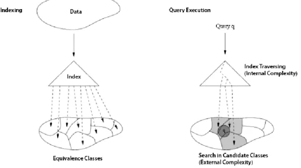
In this section, we introduce a formal model of unification. The intention is to provide a common model to analyze all the existing approaches for the proximity search. The conclusions of this section may be summarized in Figure 2. All the indexing algorithms part the set U into subsets.

An index which allows to determine a collection of candidate sets whose items are relevant to the query is constructed. At the execution time of the query, the index is scanned in search of relevant subsets (the cost of this is called "internal complexity") and these subsets are checked exhaustively (this corresponds to "external complexity" of the search).

Figure 2 - A unified model for indexing and query execution of metric spaces, equivalence Relations and Co-sets.

Given a set X, a partition (X) = {,,} is a subset of P(X) (parts of X) such that

each element belongs exactly to one partition. A relation, denoted by  is a subset of the Cartesian product X X (the set of ordered pairs) of X. Two elements x, y will be

related, and this is denoted by x y, if the pair (x, y) is present in the subset. A relation is called equivalence if it satisfies, for all x, y, z X, the reflective (x x), symmetric (x yy x) and transitive (x y y  z  x z) property.

It can be shown that each partition induces a relationship of equivalence , and vice versa, every equivalence relation induces a partition [25]. Therefore, two elements are related if they belong to the same partition. Each element  of the partition is then

called class of equivalence.

Given the set X and the equivalence relation , the set quotient (X) = X /  can be obtained, which indicates the set of equivalence classes or the cosets, obtained by applying the equivalence relation to the whole X.

The importance of equivalence classes in this study is represented by the possibility of using them on a metric space so as to derive a new metric space from the quotient set. This new metric space is more coarse than the original.

2.7 Indexes and Partitions

The equivalence classes obtained through an equivalence relation of a metric space can be considered as objects of a new metric space, as soon as a distance function on this new metric space is defined.

We then introduce the function D0 :  (X)  (X)  R, now established in quotient set.

Unfortunately this function does not satisfy the triangular inequality, so is not suitable for indexing. However, we can use any distance D that satisfies the properties of metric spaces and which is limited by D0 (e.g. D([x], [y])  D0 ([x], [y])). In this case we call D

an extension of d. Since D is a distance, it follows that (X / , D) is a metric space and therefore we can perform queries in a co-set in the same way we perform it in a set. Thus, we can convert a search problem in another, possibly easier to solve. For a given query (Q, r)d, first we find the equivalence class to which q belongs (let it [q]. Then,

using the new function D, the query is transformed into ([q], r) D. Then, we just run an exhaustive search on the candidate list (now using the original distance), to obtain the result of the query (q, r)d. The above procedure is used in virtually all the indexing

algorithms. In other words:

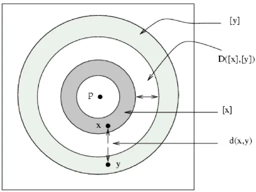
All existing indexing algorithms for proximity search consist in building the equivalence classes, discard some, and exhaustively search in the remaining. As seen briefly above, the most important compromise in the design of the partition of equivalence is to balance the cost to find [q] and check the final list of candidates. In Figure 3 we can see a schematic example of this idea. We divide the space into different regions (equivalence classes). The objects within each region are indistinguishable. We can consider them as elements of a new metric space. To find the result, rather than examine exhaustively the whole dictionary, we examine only the classes that contain potentially interesting objects. In other words, if a class can contain an element that can be returned from the query result, then the class will examined (see also the rings considered in Figure 3).

Figure 3 - Two points x and y, and their equivalence classes (colored rings). D returns the minimum distance between the rings, which represents the lower bound for the distance between x and y.

2.8 Efficiency measures

As stated previously, many of the ranking algorithms depend on the construction of an equivalence class. The corresponding search algorithms consist of two parts:

1. Find the classes that are relevant to the query

2. Examine in exhaustive mode all the elements of those classes

The first part is linked to the evaluation of certain distances d, and can also require extra CPU time. Distance evaluations performed at this stage are internal calls, and their sum defines the external complexity. The second part is about comparing the query with the list of candidates. These evaluations of d are called external and give rise to external complexity, which is linked to the discriminating strength of distance D.

We define the discriminating strength as the ratio between the number of objects in the list of candidates and the actual output of the query q, averaged over all q  X.

Note that this depends on the search radius r. Discriminating force serves as an indicator of the efficiency and appropriateness of the equivalence relation (or in correspondence, the distance function D). In general, to have a greater discriminating force will result in a greater costs in terms of internal assessments. Indexing schemes need to balance the complexity of the search for the relevant classes and the discriminating force of D.

2.9 Location of a partition

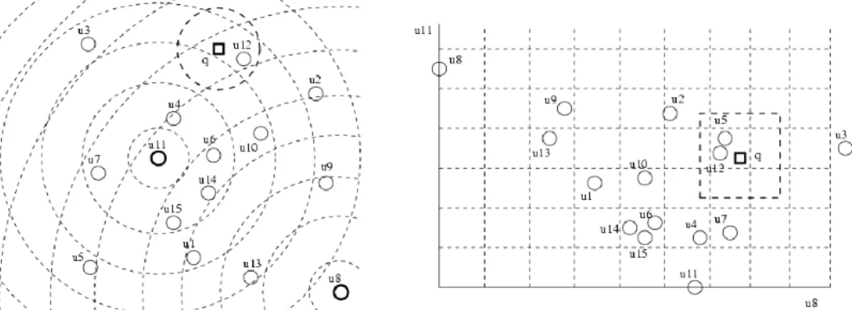
Equivalence classes can be imagined as a set of cells that do not intersect in space, where each element within a given cell belongs to the same equivalence class [10]. However, the definition of equivalence class is not confined to a single cell. One consequence of this is that you need an additional property that will be called location, whose meaning is “how the equivalence class resembles a cell”. A partition is nonlocal in cases where classes are partitioned (see Figure 4) embracing a non-compact area in space.

It is natural to expect greater efficiency, e.g. more discriminating power, from a partition that is local to a non-local one. This is because in a non-local partition the list of candidates obtained with the distance D will contain elements far enough away from the query.

Figure 4 - An equivalence relation induced by the intersection of rings centered in two pivots, and how the query is processed.

Note that in Figure 4 the fragmentation disappears as soon as we insert the third pivot. In a vector space with k dimensions, it suffices to consider k + 1 pivot in general position1 to obtain a local partition. This applies also for general metric spaces. However, to obtain local partitions is not enough: even considering local partitions assuming uniformly distributed data, we will verify that inevitably some cells remain empty, whose number grows exponentially with the space size.

2.10 Intrinsic Dimension

As explained, one of the reasons for the development of search algorithms for general metric spaces is the existence of the so-called high dimensionality. It because the traditional indexing techniques for vector spaces depend exponentially on the size of the space. In other words, if a space vector has a large number of coordinates, then an indexing algorithm that uses explicit information on the coordinates (such as kd-tree) requires exponential time (in terms of size) for answer the query. This has motivated research on the so-called indexing algorithms based on distance, which does not use explicit information on coordinates. This works very well in some vector spaces of apparently high dimension but actually small. An example is a 5-point set with the last three coordinates that are always equal to zero, or a more sophisticated case where the points lie in a 2-dimensional plane immersed in a 5-dimensional space. However, it is

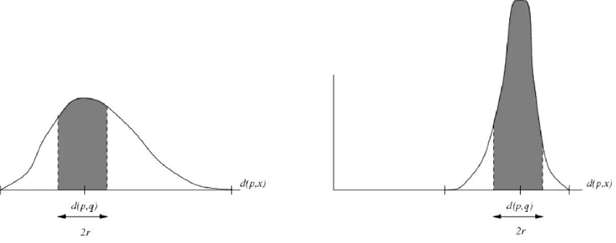
also possible that data may have a high intrinsic dimensionality. The concept of high dimensionality is not exclusive of vector spaces, but it can be characterized in metric spaces. If a vector space has an intrinsically low dimension, then considering it as a metric space can be advantageous, while for a high-dimensional vector space, the corresponding metric space in each case will be intractable. The following describes the effect of high dimensionality, and why it makes the problem intractable [22]. Let us consider the distance histogram between objects in the dictionary. This information is mentioned in many articles, in particular [16, 27]. Fixed a u element of the dictionary, let us consider the histogram of the distances d (u, ui), ui U. It is clear that the number

of elements within (u, r) d is proportional to the area under the histogram, from 0 to r

included. Now, if we calculate the histogram considering all possible pairs d(ui, uj), the

area described above is proportional to the average number of elements provided for a query of radius r.

It is reasonable to assume that the queries are distributed according to the same laws which rule the elements of the dictionary. In other words, the distribution of the distances between the query and the elements of the dictionary appears as the histogram calculated for the data set. For the search range algorithm, if we select a ring having its center in the element u*, with radii d(u*,q) – r e d(u*, q) + r, the ratio of elements captured in the ring is, on average, approximated by the area under function density in the range [d(u*,q) - r, d(u*,q) + r]. For each pivot-based algorithm, the value of the above described area governs the behavior of the algorithm itself. At each step the number of deleted items is proportional to 1 - nr. If nr = 1 then there is no elimination.

We now show that in some cases we can infer that the discriminating force of the algorithm may be very low. Let us assume that the interval where the function density is greater than zero is [ra, rb]. We note that:

1. ra is the average distance between a given element and its closest element.

2. rb is the average distance between a given element and its farthest element.

3. If r < ra, then the expected number of items in the dictionary within a sphere

centered on the query with radius r is zero. Moreover one can prove the following property:

This property is a coarse measure of the dependence on the size in algorithms based on the pivot. In the Euclidean spaces Rk, the distribution of distances between two random points becomes more "average" and has less variance in k increases. Therefore, the histogram of distances is "stretched" towards right (Figure 5), consequently stretching upwards. You can define the intrinsic dimensionality of a given metric space, considering the generic histogram shape.

Figure 5 - Histogram of distances at low number of dimensions (left) and at high scale (right), showing that for high size, virtually all elements become candidates for exhaustive evaluation.

This gives us a direct and general explanation of the problem of the so-called “curse of dimensionality”. Many authors insist on an extreme case that is a good illustration: a distance such that d(x, x) = 0 and d(x, y) = 1 for all x  y. In this way, we do not obtain any information from a comparison except that the considered element is whether or not our query. It is clear that we cannot avoid, in this case, a sequential search. The histogram of distances is totally concentrated at its maximum value. The problem of intrinsic dimensionality is also discussed in [59].

3.

Taxonomy of Searching Algorithms: K-Pole as a case of

study

In this chapter, we first organize all known approaches in a taxonomy. This will help us to identify the essential characteristics of all existing techniques, in order to find possible combinations of algorithms not yet known so far, and find out what are the most promising areas for optimization. First, we will realize that almost all algorithms are based on an equivalence relation. The intention is to group the elements of the set in cluster, so that the partitions are as local as possible and have good discriminating power. In practice, it is out that many of the algorithms used to construct the equivalence relations are based on obtaining, for each element, up to k values (also called coordinates), so that the equivalence classes can be regarded as points of a k-dimensional vector space. Many of these algorithms obtain the k values as the distances between the object and k different (and possibly independent) pivots. For this reason they are called pivoting algorithms. The algorithms differ in their pivot selection method, in when the selection is made, and how much information is used for comparisons. Figure 11 summarizes methods classification based on their most important features.

Figure 6 - Taxonomy of existing algorithms. Methods written in italics are combinations of already existing ones.

3.1 The Relation of Equivalence of Pivots

Many of the existing algorithms are built on this equivalence relation. The distances between an element and a number of preselected pivot (e.g. elements of the universe, also known in the literature as vantage points, keys, queries, etc..) are considered. The equivalence relation is defined in terms of distances between the elements and pivots, so two elements are equivalent when they are at the same distance from a pivot. If we consider a pivot p, then this equivalence relation is

xp  p y  d(x, p) = d( y, p).

The equivalence classes correspond to the intuitive notion of a family of spherical shells centered at p. Points that fall within the same sphere are those equivalent to or indistinguishable from the point of view of p. The equivalence relation above is easily generalized to k pivots or reference points pi to obtain

and in the general case a graphical representation of the partition corresponds on intersection of different spheres centered at the points pi. Alternatively, we can consider

the equivalence relation as a projection of the Rk vector space, being k the number of used pivot. The i-th coordinate of an element will be the distance between the element and the i-th pivot. Once that is done, we can identify points in Rk with elements in the original space with the L distance. The indexing algorithm then consist in searching the

set of equivalence classes such that they fall within the search radius. A third way to see the technique, less formal but more intuitive, is the following: to check whether an item uU belongs to the query result, we prove a number of random pivot pi. If, for each of

these pi, we have |d(q, pi) - d(u, pi )| > r, then the triangle inequality assures us that d (q,

x) > r without the need for calculate the values of d(q, pi). The only u elements that

cannot be discarded through the use of pivot will be the only ones compared directly with the query object q.

3.2 Selecting Pivots

We must find the optimal number for the k pivot. If k is too small, then finding the classes will be inexpensive, but the partition will be very coarse and probably not local, and we will pay a high price during the exhaustive search. If k is too large then the partitions will be less expensive to traverse, but the cost for calculate them will be high. The number of pivot we need to obtain a good partition is linked to the intrinsic dimension of the data set. In [33] is formally proved that if the size is constant, then after selecting a proper constant number k of pivot, exhaustive search costs O(1) (but their theorems don’t show how to select the pivots). In AESA [55], we show empirically that O(1) pivot are required for this result, then we will have a total O(1) search time (their algorithm is not practical). On the other hand, in [6], it is shown that O(log n) pivots are needed to have a comprehensive final cost of O(log n). This difference is due to different models of the space structure (e.g. finite volume) and statistical behavior of the distance function. The correct answer probably depends on the considered particular metric space. A related topic is how to select the pivot. All current schemes select the pivots randomly from the set of objects U. This is done for simplicity, although addressing this issue could have notable improvements. For example, in [51] is recommended to select the pivots outside the cluster, while in [5] is suggested to use a pivot for each cluster. All authors are agreed that the pivot should be

away from each other, and this is obvious since pivot close to each other would lead almost the same information. On the other hand, pivot randomly selected are probably far enough in a high dimensional space. To discriminate a compact set of candidates, a good idea is to select a pivot between these same candidates. This makes it more likely to select an element next to them (ideally select the centroid). In this case, distances tend to be few. For example, LAESA[42] does not use pivots in fixed order, but the next to be selected will be the one with minimum distance L1 from the current candidates.

3.3 Search Algorithms

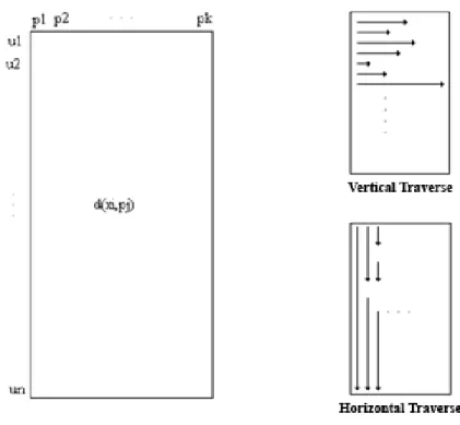
After determining the equivalence relation to use (e.g. k pivot), the set undergoes a preprocessing where there are stored, for each element of U, its k coordinates (e.g. the distances from the k pivots). It involves a preprocessing of cost O(kn), both spatial and temporal. The index can be seen as a table of n rows and k columns as shown in the left part of Figure 7.

Figure 7 - Schematic view of a pivot based indexing, in vertical and horizontal traverse When query is executed, it is first compared with the k pivots, thereby obtaining its k coordinates (y1, ..., yk) in the target area. It corresponds to determine which equivalence

complexity of the search. It must be then determined, in the target space, which equivalence classes may be relevant to the query (e.g. which are at a distance r or less in the metric L, which corresponds to the distance D). This does not involve additional

distance evaluations, but produces an extra cost of CPU time. Finally, the elements that belong to the qualifying classes (e.g. those who cannot be discarded after considering the k pivot) are directly compared with q (external complexity). The simplest search algorithm proceeds line by line: it considers each item in the collection (e.g. each row (x1, ..., xk) of the table) and sees if the triangle inequality allows to discard that row, i.e.

if max i=1..k{|xi - yi|}> r . For each row that is not rejected by applying this rule, the

elements are directly compared with q. Although this type of crossing does not perform most of the necessary evaluations of d, is not the best choice. First, note that the amount of CPU work is O(kn) in the worst case. However, if we leave a line when we find there is a difference bigger than r scanning the coordinates, the average case is closer to O(n). The first improvement consists in processing the whole set column by column. Therefore, we compare the query with the first pivot p1. Now, consider the first column

of the table and discard all the elements that satisfy |x1 - y1| > r. Then consider the

second pivot p2 and repeat the procedure only on not previously discarded items. An

algorithm that implements this idea is the LAESA. It is not difficult to see that the number of distance evaluations and the total CPU work remain the same as the line by line case. Anyway, now we can do better because each column can be sorted so that the interval of the qualifying rows can be traversed in binary mode instead of sequential mode[45, 23]. This is possible because we are interested, at column i, in values [yi - r, yi

+ r]. This is not the only allowed “trick” from a column for column evaluation (which cannot be done in the line by line case). A very important trick is that it is not necessary to consider all the k coordinates. As soon as the set of remaining candidates is small enough, we can stop considering the remaining coordinates and directly verify the candidates using the distance d. This point is difficult to determine in advance: despite the (few) existing theoretical results [33, 6], usually the application cannot be understood well enough to predict the optimal number of pivots (e.g. the point where it is better to switch to the comprehensive assessment). Another trick that can be used with the column for column evaluation is that the selection of the pivot can be done "on the fly" rather than before. In this way, once you select the first pivot p1 and discard all

the not interesting elements, the second pivot p2 may depend on which has been the

the elements with respect to this pivot. In this way, we select k potential pivots and operate a preprocessing work on the table like before, but now we can choose in which order to use the pivots (according to the state current research) and where to stop the using of pivots and go to compare directly. An extreme case of this idea is AESA, where k = n, i.e. all the elements are potential pivots, and at each iteration the new pivot is randomly selected among the remaining elements. Despite its inapplicability in practice because of the time (and space) preprocessing of order O(n2) (because distances between all the known elements are precomputed), the algorithm calculates a surprisingly low number of distances, even better when the pivot is fixed at first. This shows that it is a good idea to select the pivots from the current set of candidates. Finally, we note that instead of a sequential search in an mapped area, we could use a search algorithm for k-dimensional vector spaces (e.g. kd-trees or R-trees). According to their ability to handle large values of k, we may be able to use more pivots without significantly increasing the CPU cost. It should be remembered also that, when many pivots are used, research facilities working worst for vector spaces. This is a very interesting problem that has not been studied further, that considers the balance between distance computations and CPU time.

3.4 Comparisons between existing Data Structures

Comparisons performed on various existing data structures show that, using the same amount of memory, BKT is the most efficient data structure, followed for higher dimensions by other similar schemes. In addition it was found that, for areas of high size, techniques based on Voronoi partitions [3, 58] have proved more efficient than those based on pivots. On the other hand, FHQA, FMVPA and LAESA have the characteristic of improving their performance by using multiple pivot. LAESA requires an amount of memory 128 times greater and FHQA and FMVPA require 32 times more memory than the LAESA amount, in order to be capable of beating BKT in 20 dimensions spaces. It is interesting to note that, with increasing size, pivoting algorithms need more pivots to beat the algorithms based on Voronoi partitions. On the other hand, there are no good methods that allow Voronoi-like algorithms to use more memory to increase their efficiency, but if there were, they likely would require less space to obtain the same results of other algorithms in spaces of higher dimensions. Note also that only the implementations for arrays of FHQT and FMVPT make possible

in practice the amounts needed for the calculations. We believe that a data structure that combines the idea of Voronoi partitions with an k-pivoting algorithm may represent the best compromise.

3.5 Considerations and Open Problems

Many of the existing algorithms are in fact based on variations of a few ideas, and identifying them, have appeared combinations not known before, and some of they were particularly efficient. We can summarize the path showed so far with the following statements:

1. The factors which affect the efficiency of a search algorithm are the intrinsic dimension of space and recovered proportion of the whole set (in percent). 2. We have identified the use of equivalence relations as the common ground that underlies all the indexing algorithms, and classified the search cost in terms of internal and external complexity.

3. A broad class of search algorithms depend on the selection of k pivots and the mapping of the metric space on Rk, using the distance L. Another important

class of algorithms use the Voronoi partitions.

4. Although there is an optimum number of pivots to use, this number is too high in terms of space requirements. Therefore a compromise between the number of pivots and requirements the system.

5. Algorithms based on Voronoi partitions are more resistant to the increase of the intrinsic size of the space.

6. Among the considered structures, experimental results show that the best one is the version of BKT adapted to continuous spaces of arity 2. This structure "degenerates" into a very efficient clustering scheme. If the availability of memory increase, at the end other structures will be better of BKT. Among these, those which best use memory are FHQA and FMVPA.

But there are a number of open issues that require further attention. The main are listed below: