Bi-directional exchange of greenhouse gases and pollutants between a Mediterranean holm oak forest and the atmosphere

- 2016 –

UNIVERSITÀ DEGLI STUDI DELLA TUSCIA DI VITERBO

Department for Innovation in Biological, Agro-Food and Forest Systems

DIBAF

PhD in Forest Ecology, cycle XVIII

Bi-directional exchange of greenhouse gases and pollutants

between a Mediterranean Holm oak forest and the atmosphere

BIO/07

Candidate

Supervisor

Flavia Savi

dr. Silvano Fares

PhD Coordinator

Contents

List of tables ... iii

List of figures ... iv

Main symbols and abbreviations ... vi

Abstract ...ix

List of scientific publications produced during the PhD course ...xi

1 Introduction ... 1

1.1 Greenhouse gases and atmospheric pollutants ... 1

1.1.1 Carbon Dioxide ... 1

1.1.2 Methane ... 2

1.1.3 Tropospheric Ozone ... 3

1.1.4 Volatile Organic Compounds... 5

1.1.5 Nitrogen Oxides ... 7

1.2 Atmospheric pollution effects on forest ecosystems ... 7

1.3 Thesis overview and structure ... 10

2 Methods ... 12

2.1 The study site ... 12

2.2 Micrometeorological methods ... 14

2.2.1 Eddy covariance technique for flux measurements ... 15

2.2.2 Inverse Lagrangian technique to evaluate source / sink distribution within the forest canopy ... 17

2.2.3 Resistance modelling of O3 deposition ... 18

2.2.4 Measurements and instrument set-up ... 22

2.3 Statistics ... 24

2.3.1 Multiple Linear Regression ... 24

2.3.2 Partial Least Squared Regression ... 26

2.3.3 Singulars Spectrum Analysis ... 26

2.3.4 Feed Forward Back-Propagation Artificial Neural Network ... 28

3 Carbon balance at the forest ... 32

3.1.1 CO fluxes and their dependence from meteorology and phenology ... 32

3.2 CH4 exchanges at the forest ... 34

3.2.1 CH4 mixing ratio above the forest ... 35

3.2.3 CH4 fluxes above the forest ... 36

3.2.4 Environmental and biological controls on CH4 exchange ... 39

4 Ozone deposition and uptake by vegetation ... 50

4.1 O3 mixing ratio above the forest ... 51

4.2 Above canopy O3 fluxes ... 52

4.3 Partitioning of O3 deposition between its sinks at the forest ... 53

4.3.1 O3 stomatal sink ... 53

4.3.2 O3 deposition to soil: below-canopy EC measurements and modelling ... 57

4.3.3 O3 deposition to cuticles ... 61

4.3.4 Gas-phase reactions ... 61

4.4 Dependence of forest O3 uptake from water availability ... 64

5 Ozone effects on Net Ecosystem Exchange ... 68

5.1 Testing the ozone effect on NEE using the Artificial Neural Network approach ... 68

5.1.1 Preparation of the dataset ... 68

5.1.4 Contributions of the input variables in the ANN prediction process ... 72

5.2 Testing the ozone effect on NEE using Partial Least Square approach... 76

6 Synthesis and overall discussion ... 80

Conclusions ... 84

Acknowledgements... 86

List of tables

Table 1 ... 13

Table 2 ... 42

Table 3 ... 43

Table 4 ... 44

Table 5 ... 45

Table 6 ... 55

Table 7 ... 59

Table 8 ... 77

Table 9 ... 77

List of figures

Figure 1.1

Effects of O

on plant processes at the cellular, leaf, whole-plant,

and community scales.. ... 9

Figure 1. 2

Diagram of the PhD work activities and their relations with the

thesis objectives. ... 11

Figure 2. 1

Study site locationd. ... 12

Figure 2. 2

Resistance deposition model for O

... 19

Figure 2. 3

Example of an ANN structure ... 29

Figure 3. 1

aily CO

exchange recorded above and below canopy, monthly

precipitation and monthly mean temperature. ... 33

Figure 3. 2

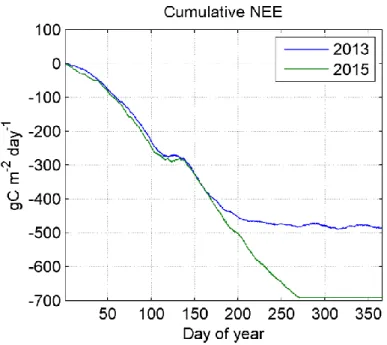
Cumulative NEE for 2013 and 2015 ... 34

Figure 3. 3

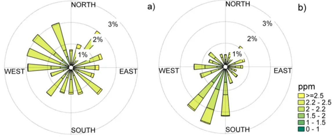
Wind roses of Autumn-Winter and Spring-Summer wind

directions and CH

mixing ratio ... 35

Figure 3. 4

Daily course of above canopy CH

mixing ratio ... 36

Figure 3. 5

Dynamic of CH

fluxes above canopy ... 37

Figure 3. 6

Daily distribution of raw, WPL corrected CH

fluxes and fully

filtered CH

fluxes. ... 38

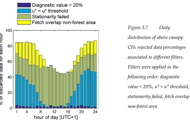
Figure 3. 7

Daily distribution of above canopy CH

rejected data percentages

associated to different filters ... 39

Figure 3. 8

Relative importance of each predictors within the PLS models. ... 41

Figure 3. 9

Ratio of methanogens and methanotrophs abundance over the soil

CH

-cycling communities and per cent distribution within the layers ... 47

Figure 4. 1

Surface-plot of O

mixing ratio... 51

Figure 4. 2

Wind roses of Day-time and Night-time wind directions and O

mixing ratio

... 52

Figure 4. 4

Mean daily evolution of air temperature, vapour pressure deficit,

total and stomatal O

fluxesfor the each season of the year 2013. ... 57

Figure 4. 5

Daily mean evolution of total O

fluxes measured above the

canopy, below the canopy, modelled according to the empirical modeland

modelled according to the resistance method ... 60

Figure 4.6

Surface plot of NO and NO

mixing ratio vertical profile, averaged

for the hour of day. ... 62

Figure 4.7

Mean daily evolution of NO, NO

and O

deposition velocity,

modelled through ILT. ... 62

Figure 4.8

Source / sink distribution along a soil-canopy profile of

mototerpenes. ... 63

Figure 4.10

Cumulative precipitation recorded in Early Spring and Late

Autumn during 2012 and 201 ... 64

Figure 4. 11

Mean daily course of ait temperature, latent heat flux, vapour

pressure deficit and O

deposition velocity recorded during Early Spring and

Late Autumn in 2012 and 2013 ... 65

Figure 5.1

NEE decomposition through SSA ... 70

Figure 5. 2

ANNs structure. ... 71

Figure 5. 3

Boxplot comparing measured and modelled NEE. ... 72

Figure 5. 4

Results from the connection weight analysis. ... 73

Figure 5.5

Partial derivative of NEE with respect to F

, plotted against

F

74

Figure 5. 6

Scatterplot of NEE increase for a [O

] reduction of 30 %. ... 75

Figure 5.7 Daily mean evolution of NEE reduction due to O

effects, stomatal O

uptake and stomatal conductance. ... 75

Figure 5.8

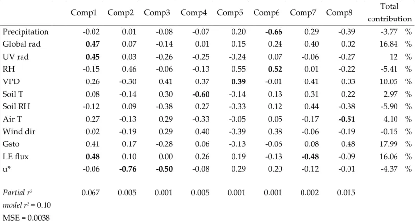
Relative importance (%) of each predictors within the PLS model ... 78

Figure 5.9

Plot of swc

vs PAR (photosynthetic active radiation. ... 79

Main symbols and abbreviations

Symbols Description Unit or

Value of Costants

Latin alphabet

B Stanton number ꟷ

cp Specific heat capacity of air 1246 J kg-1 K-1

d Displacement height m

D Dispersion matrix s

Dx molecular diffusivity of a gas

E Latent heat flux kg m−2 s−1

Fg Ground flux (at z=0) mmol m-2 s-2

μmol m-2 s-2 nmol m-2 s-2

FO3sto O3 stomatal uptake nmol m-2 s-2

Fx Flux of a gas mmol m-2 s-2

μmol m-2 s-2 nmol m-2 s-2

g Gravitational acceleration 9.81 m s-2

GO3 Stomatal conductance to O3 mol m-2 s-1

Gst Stomatal conductance to H2O mol m-2 s-1

H Sensible heat flux °K m-1 s-1

H2OfluxAC H2O fluxes above canopy mmol m-2 s-2

H2OfluxBC H2O fluxes at ground level mmol m-2 s-1

hc Canopy height m

hv Light ꟷ

k Von Karman constant 0.41

KH Eddy diffusion coefficient m2s-1

L Monin-Obukhov length m

LE Latent heat flux W m-2

prec Precipitation mm

qa vapour pressure kg kg−1

qs saturation mass fraction of H2O at air temperature

kg kg−1

Ra Aerodynamic resistance s m-1

rad Global solar radiation Wm-2

Rb Laminar boundary layer resistance s m-1

Rc Canopy resistance s m-1

Rct(dry)0 reference value for Rct calculation in dry condition

6000 s m−1

Rct(wet)0 reference value for Rct calculation in wet condition

400 s m−1

Re Reynolds number ꟷ

Rg Ground resistance s m-1

Rg1 Constant resistence for Rg calculation 50 s m−1

Rg2 Constant resistence for Rg calculation 500 s m−1

RH Relative humidity %

RH soil 10 Soil relative humidity 10 cm depth %

RH soil 100 Soil relative humidity 100 cm depth %

RH soil 50 Soil relative humidity 50 cm depth %

Rs Stomatal resistance to H2O s m-1

S Suorce or sink strength μmol m-2 s-2

nmol m-2 s-2

Sc Schmidt number ꟷ

swc Soil water content %

swc10 Soil water content measured at 10 cm depth %

swcfc Soil water content measured at field capacity 28%

T air temperature °K

T air Air temperature °C

T soil 10 Soil temperature 10 cm depth °C

T soil 100 Soil temperature 100 cm depth °C

T soil 50 Soil temperature 50 cm depth °C

TL Lagrangian time scale s

u Horizontal wind velocity m s-1

u* Friction velocity m s-1

UV Ultraviolet radiation (280-360 nm) Wm-2

v Lateral wind velocity m s-1

va kinematic viscosity of air m2 s -1

Vd Deposition velocity m s-1

w Vertical wind velocity m s-1

wh ANN connection weight between input and

hidden neurons

ꟷ

winddir Wind direction °

wo ANN connection weight between hidden and

output neurons

ꟷ

z Measurement height m

z0 Roughness length, mean hight above d at

which momentum is absorbed

m

Concentration of a gas ppm ppb

Xfar _{Concentration due to far-field effect ppm}

ppb

Xnear _{Concentration due to near-field effect ppm}

ppb

β _{Regression coefficient} ꟷ

γ _{Psychrometric constant 4.08 ×10}−4 _K−1

ε _{Regression intercept} ꟷ

ζ _{Stability parameter} ꟷ

λ _{Vaporisation heat for H}2O 2.5×106 J kg−1

ρa _{Density of dry air 1.01 g m}-3

σw _{Standard deviation of vertical wind velocity m s}-1

ΨH _{Stability correction function for heat} ꟷ

ΨM _{Stability correction function for momentum} ꟷ

Abbreviations Description

ANN Artificial Neural Network

AVOC Anthropogenic Volatile Organic Compound

BVOC Biogenic Volatile Organic Compound

EC Eddy Covariance technique

ES Early Spring - Mar 20th _{to Apr 14}th _period

ILT Inverse Lagrangian technique

KS Kolmogorov-Smirnov test

LA Late Autumn - Nov 11st _{to Dec 6}th _period

OVOC Oxygenated volatile organic compound

PCA Principal Component Analysis

PLB Planetary Boundary Layer

PLS Partial Least Square regression

ROS Oxigen Reactive Species

SSA Syngular Spectrum Analysis

Abstract

Forests play a major role in regulating air quality and climate. However, plant exposure to atmospheric pollution may cause detrimental effects on vegetation. Among others,

tropospheric O3 is probably the most damaging to forest ecosystems: entering the leaves thought stomata, it causes oxidative stress and damages photosynthetic apparatus, reducing carbon assimilation. This PhD work aimed to quantify fluxes of greenhouse gases (CO2, CH4, O3) in a Mediterranean holm oak forest located near Rome (Italy) exposed to high levels of tropospheric O3 concentration. A primary goal was also to evaluate the O3 damage on the forest carbon assimilation capacity.

Four years of eddy covariance measurements demonstrated that the ecosystem is an active CO2 sink all year long (485 – 690 g C m-2 y-1). For the first time, long term monitoring of CH4 exchange above a Mediterranean forest showed that the ecosystem is a net CH4 sink during the cold season and a net source during the dry season, thus making the annual net CH4 exchange close to the neutrality.

Precipitation events during Summer season have been found to be one of the most important factors controlling carbon exchanges at the forest, thus influencing the CO2 uptake and the magnitude of the CH4 emission. The dry condition in Summer period depressed CH4

-oxidizing bacteria, so that the ecosystem acted as a net source of CH4 in this period, thanks to translocation of CH4 from the soil to above canopy through xylematic pathways.

Furthermore, the Summer high UV radiation has been found to promote CH4 production from photochemical reactions on leaves waxes, thus contributing to the overall strength of the Summer CH4 emissions.

Besides being a sink for carbon, the holm oak forest represents a net sink of O3. The annual budget has been estimated around 80 mmol m-2 _y-1_{. The major sink were stomata, being O3} uptake strongly connected to the physiological plant activity and subject to water

The influence of O over NEE was tested using a novel approach, which combines non parametric time series decomposition and the explanatory capacity of Artificial Neural Networks. Results suggested that O3 has a detrimental effect over NEE during Spring and Summer seasons, although the magnitude of this reduction is low (rate of reduction of NEE for unit change of O3 stomatal uptake = 0.015).

The results of this PhD work demonstrated that this Mediterranean forest is an active carbon sink and contributes to ameliorate air quality removing O3 from the atmosphere. However, O3 uptake through stomata reduces carbon assimilation, although it does not represent the main limiting factor to forest productivity as compared to drought. The latter showed to be the major limiting factor at the forest leading to strong reduction of CO2 assimilation, enhancement of CH4 emission and limitation to O3 uptake. These results help to foresee possible future effects of climate change and pollution on Mediterranean forest ecosystems.

List of scientific publications produced during the

PhD course

Published papers:

Fares S., Savi F., Muller J., Paoletti E., Matteucci G., 2014. Simultaneous measurements of above and below canopy ozone fluxes help partitioning ozone deposition between its various sinks in a Mediterranean Oak Forest. Agricultural and Forest Meteorology, 198-199:181-191. DOI: 10.1016/j.agrformet.2014.08.014

Savi F., Fares S., 2014. Ozone dynamics in a Mediterranean Holm oak forest: comparison

among transition periods characterized by different amounts of precipitation. Annals of Silvicultural Research, 38(1):1-6. DOI: 10.12899/asr-801

Aromolo R., Savi F., Salvati L., Ilardi F., Moretti V., Fares S., 2015. Particulate matter and meteorological conditions in Castelporziano forest: a brief commentary. Rend. Fis. Acc. Lincei 26 (3): 269-273. DOI: 10.1007/s12210-015-0414-5

Accepted paper:

SaviF., Di Bene C., CanforaL., MondiniC., FaresS., Environmental and biological controls

on CH4 exchange over an evergreen Mediterranean forest. Agricultural and Forest Meteorology.

Submitted papers:

Canfora L., Di Bene C., Savi F., Migliore M., Farina R., Fares S. Evaluating factors

influencing soil microbial communities and CO2 exchanges in a Mediterranean Holm oak forest. Submitted toEnvironmental Monitoring and Assessment.

Fares S., Savi F., Fusaro L., Conte A., Salvatori E., Aromolo R., Manes F. Particle deposition in a peri-urban Mediterranean forest. Submitted to Environmental Pollution.

1

Introduction

Forests play a major role in regulate air quality and climate. Beside fixing carbon dioxide trough photosynthesis, vegetation controls other greenhouse gases and pollutants transport across the forest-atmosphere boundary. This control is expressed primary by three principal mechanisms: dry or wet surface deposition, stomatal uptake and gaseous phase reactions. Leaves and branches provide a surface much bigger than the corresponding soil surface, air spaces inside the stomata increase the available surface where gases deposit or dissolve. Many physiological processes involve gases for chemical reactions within or outside the leaves, such as antioxidant systems in the cell walls or the emission of volatile organic compounds.

However, plant exposure to atmospheric pollution may cause detrimental effects that weaken vegetation carbon sink potential. Although pollution does not represent the main limiting factor to forest productivity as compared to other environmental factors such drought or lack of nutrients, its effect on Mediterranean vegetation is of particular concern. Indeed, the strong anthropic pressure on densely inhabited Mediterranean coasts, together with the occurrence of climatic conditions that promote pollutants formation through photochemical reactions, represents a great stress factor for vegetation.

1.1

Greenhouse gases and atmospheric pollutants

1.1.1 Carbon Dioxide

Atmospheric carbon dioxide (CO2) is the second most abundant greenhouse gas in the atmosphere after water vapour (H2O), with a radiative forcing of 1.69 Wm-2 (Shindell et al., 2009). Its concentration has substantially increased since the industrial revolution began in the 19th _{century, mainly due to anthropogenic activity. Three quarter of anthropogenic CO2}

emissions is attributed to fossil fuel combustion, followed by deforestation and land-use change (Brugnoli and Calfapietra, 2010).

Forests represent the major land biosphere sink of CO2 (Melillo et al., 1993), which depends on the balance between photosynthetic fixation and CO2 release by autotrophic respiration and biomass decomposition. This equilibrium presents a strong temporal variability at different scales (diurnal, seasonal, annual) and it is controlled by climate and by length of the growing season (Valentini et al., 2000).

Forest ecosystems net absorption of CO2 is called Net Ecosystem Exchange (NEE) and is generally measured on annual scale. NEE represents the amount of carbon subtracted from the atmosphere and stored in live biomass, litter and soils. Although NEE is commonly positive, that is ecosystems subtract carbon from the atmosphere, in some cases is observed a net release of CO2 from forests, imputable to many factors that enhance respiration, between them, climate variations end disturbance regimes (Rice et al., 2004; Williams et al., 2014). Mediterranean evergreen forests ensure CO2 sequestration and storage all year long, although the CO2 absorption rate changes among seasons depending on temperature and water availability, which represent the main environmental stress in this region. High temperature and drought re-occur cyclically every year in Summer and natural selection processes made Mediterranean vegetation adapted to these environmental conditions. Although, when natural stress factors are coupled with anthropogenic pollution, forest carbon sequestration potential can decrease.

1.1.2 Methane

Methane (CH4) is the most abundant hydrocarbon and the third greenhouse gas in the atmosphere after H2O and CO2. Its global warming potential (over 100 years) is 28-36 times higher compared to CO2 (IPCC, 2013) and its indirect effect on aerosols and other chemical compounds by altering the atmosphere oxidative capacity (Shindell et al., 2009) make this gas of particular concern.

CH4 concentration increased by 2.5 times since pre-industrial time (Etheridge et al., 1992). Both natural sources, i.e. wetlands, and anthropogenic activities, i.e. biomass burning, fossil fuel production, livestock and rice paddies, contribute to CH4 global source (Denman et al., 2007), estimated at 600 T CH4 y-1 (Lelieveld et al., 1998).

In forest ecosystems, soil is the primary compartment where CH4 exchange takes place: methanotrophic and nitrifying bacteria are responsible for atmospheric CH4 uptake, whereas emission is regulated by metanogenic archaea, strictly limited to anaerobic environments (Trotsenko and Khmelenina, 2002). Recently, studies have suggested a contribution of forest vegetation to CH4 emission (Keppler et al., 2006), although the significance of this emission is still under debate (Bruhn et al., 2012; McLeod et al., 2008). The main mechanisms explaining CH4 release from vegetation are: contribution via the transpirational stream through the xylem (Zeikus and Ward, 1974), anaerobic source in the trunk (Mukhin and Voronin, 2011), induction by UV radiation and heat from plant tissues (McLeod et al., 2008; Vigano et al., 2008), wounding (Wang et al., 2009), or reactive oxygen species induction (Sharpatyi, 2007; Vigano et al., 2008).

Few studies were conducted over forests ecosystems contribution to the CH4 biosphere – atmosphere exchange (Nicolini et al., 2013) and none of them was conducted over a Mediterranean forest. Literature highlights that CH4 flux magnitude over different forest types is widely variable, depending on forest and soil types, and even the direction of fluxes can change, reacting to different meteorological variables. This variability is mainly due to microbial responses to environmental factors influencing microbial activity such as

meteorological conditions, soils texture, N availability and salinity (Stams and Plugge, 2010). Due to their role in controlling CH4 behaviour, the understanding of soil microorganisms involved in the CH4 cycle represents a cognitive platform for any CH4 study aimed to

explore the connection between ecosystems and CH4 fluxes.

1.1.3 Tropospheric Ozone

Tropospheric ozone (O3) is a secondary pollutants, mainly produced through photochemical reactions of methane (CH4), carbon monoxide (CO), and volatile organic compounds (VOC)

in the presence of nitrogen oxides (NOx). A minor O3 source is the downward transport from the stratosphere (Junge, 1963). Is the third greenhouse gas in the atmosphere, and contributes to the climate change with a radiative forcing of 0.35-0.37 W m-2 _{(Shindell et al., 2009). High} O3 concentrations are associated with negative effects on human health (respiratory diseases), natural ecosystems and crops (The Royal Society, 2008).

Chemistry that controls O3 production and destruction in the troposphere is summarized by the following reactions (Monks et al., 2015):

NO2 + hv  NO + O (1)

O + O2 O3 (2)

HO2 + NO  NO2 + OH (3)

O3 + NO  NO2 + O2 (4)

The above reactions do not represent a mechanism of net O3 production since the rapid interconversion between NO and NO2 leads to both O3 production and destruction. This equilibrium is altered in presence of volatile organic compounds (VOCs):

VOC + OH + O2  CO2 + HO2 (5)

VOCs oxidation produces of hydroperoxyl (HO2) , which reacts with NO, changing the [NO]/[NO2] ration, leading to O3 formation. From the above formulas arises that O3 formation depends on the balance of its precursors, which have both natural and

anthropogenic origin. In rural areas, O3 formation rate is not limited by VOCs availability and increases with NOx concentration increase (NOx limited). In urban environment, O3 formation rate increases with increasing VOCs concentration and it is inhibited by increasing NOx concentration. These chemical regimes make O3 concentration highest in rural areas located downwind of polluted cities.

Background O3 concentrations at present days is 30-40 ppb (Parrish et al., 2012), however large regional differences are recorded due to the strong influence of weather, which promotes O3 formation in warm, dry and sunny conditions.

O3 lifetime in the lower troposphere is around 5 days (Fusco and Logan, 2003). O3 photolysis is the major source of OH radicals, the primary oxidant in the troposphere:

O3 + hv  O + O2 (6)

O + H2O  OH + OH (7)

Another O3 sink in addition to the chemical destruction is the removal at the surface by dry deposition that occurs in forest ecosystems through stomatal uptake, non-stomatal uptake and in-canopy chemistry.

Stomatal uptake by vegetation allows O3 enters the leaves, thus removing this pollutant from the atmosphere. By contact with cell walls, membranes and metabolites, O3 generates free radicals within the apoplast, damaging cell metabolism (Hindawi, 1979). The main detrimental effect is carbon assimilation reduction, caused by photosynthetic apparatus damage. The O3 portion entering the stomata depends on stomatal aperture, which in turn is regulated by many environmental and physiological factors, among them: light,

temperature, CO2 concentration, vapour pressure deficit, water availability, phenology (Grünhage et al., 2012).

Non-stomatal uptake includes all the reactions of O3 with the external surface of vegetation and soil. Temperature and canopy wetness can increase reaction rates of O3 with organic compounds on leaves ( Rondón, 1993; Coyle et al., 2009). In-canopy chemistry depleted O3 concentration through oxidation of NO emitted by soil and through oxidation of VOCs emitted by vegetation.

1.1.4 Volatile Organic Compounds

Volatile organic compounds (VOCs) are trace organic gases other than CO2 and CH4. Their origin can be both biogenic (BVOCs) and anthropogenic (AVOCs). Biogenic emissions are estimate around 800 Tg C y-1 _{and exceed anthropogenic of one order of magnitude (Lathiere} and Hauglustaine, 2006). VOCs release in plants has multiple roles, linked to growth,

reproduction, defence against stresses, protection and communication (Peñuelas and Staudt, 2010).

They are involved in many reactions that affects atmospheric chemistry and carbon cycle. Almost 10 % of the carbon fixed by photosynthesis is released as VOCs by vascular plants (Llusia and Peñuelas, 2000). Once in the atmosphere, VOCs react and their products impact on O3 production or destruction (as outlined in the 1.1.2 section), aerosol production and cloud formation (Holzinger et al., 2005), airborne N deposition and acidification.

A large number of chemical groups are included within VOCs. Many of them are toxic to human and ecosystems, such as aromatic hydrocarbons, aldehydes and ketones (Burn et al., 1993; Kampa and Castanas, 2008).

Isoprenoids (isoprene, monoterpenes and sesquiterpenes) are the predominant group, followed by alcohols and carbonyls. Isoprenoids are quite reactive and their lifetime vary between minutes to hours (Kesselmeier and Staudt, 1999), they are poorly water-soluble and characterized by a strong scent. Isoprene (C5H8) represent the 50% of BVOC emissions (Guenther et al., 2000), and is produce especially by poplars, aspen, oaks and eucalyptus trees. Monoterpens (C10H16), mainly in the form of α-pinene and β-pinene, contribute to the 10-15% of emissions (Fowler et al., 2009). The outstanding part is represent by oxygenated VOC, which are less reactive than isoprenoids and ubiquitously produces by all plant species.

Depending on the species, BVOC emission can be regulate by compounds synthesis rate or by evaporation and diffusion from storage pools. Plants can also act as sink for BVOC when their air concentration is higher than those inside plants (Noe et al., 2008).

Mediterranean costal ecosystems are almost exclusively characterized by monoterpenes emitting species (Loreto et al., 1998). One of the predominant species that characterize this environment is Quercus ilex L. This evergreen oak does not store monoterpenes, so that their emissions is directly correlated with temperature and light intensity (Loreto et al., 2004), which make monoterpenes emission rates varying according to daily and seasonal cycles. This emission pattern, associated with high reaction rate with OH radicals in the atmosphere, in turn affects O3 chemistry during photochemically active periods of the year.

1.1.5 Nitrogen Oxides

Nitrogen oxides (NOx) are treated as a chemical family that include NO and NO2. The main NOx sources are fossil fuel combustion, biomass burning, soils and lightening (Seinfeld and Pandis, 2016). Almost 95% NOx emission from combustion are NO, which rapidly converts to NO2 in the atmosphere (as outlined in the 1.1.2 section). Atmospheric concentration of these compounds is highly variable, ranging between <1 ppb in remote location to 10-1000 ppb in urban areas, where the main sources are located (Von Schneidermesser et al., 2015).

NOx radiative forcing is 0.29 W m-2 (Shindell et al., 2009), and is the result of a variety of opposite interactions of NOx with other greenhouse gases, i.e. SO4, CH4, NO3, and O3. NOx relation with O3 affects NOx lifetime, which ranges from hour to days (Berntsen et al., 2005).

NOx are harmful pollutants that negatively affect human health, inducing respiratory and heart diseases (Godish et al., 2014). Negative effects of NOx on ecosystem can be direct, as acid deposition that compromises soil and water quality, or indirect, as formation of secondary pollutants such O3 and particles (Van Grinsven et al., 2013).

1.2 Atmospheric pollution effects on forest ecosystems

Vegetation role as important sink for air bone pollutants and greenhouse gases is widely recognized. On the other hand, plants are damaged by filtering air pollutants, and effects on forest ecosystems can be severe. Reduction of forest productivity represents an early detection of the forest decline, before the occurrence of visible injuries.

Manipulative experiments have been widely used to test pollution sensitivity, however such experiments have several limitations, since plants are often exposed unrealistic concentrations, young seedling, and the experimental facilities, e.g. open top chambers, impact the microclimate of the trees. For these reasons, understanding how pollution affects the CO2 uptake by open forests is of primary importance.

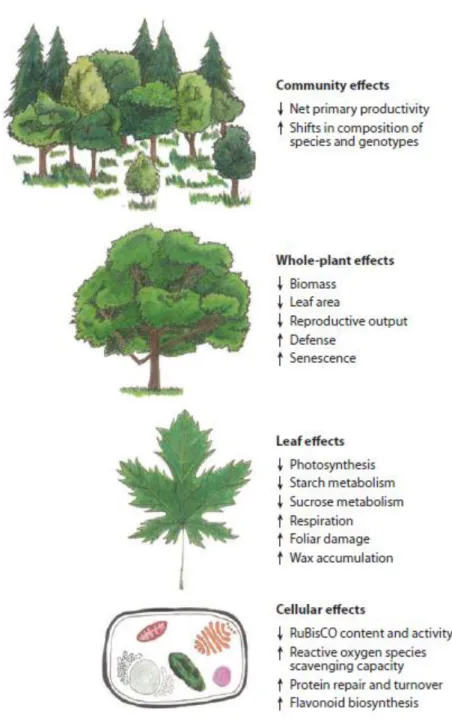
Among air pollutants, O3 is probably the most damaging to forest ecosystems (Ollinger et al., 1997). O3 phytotoxicity derives from the oxidative damages it produces inside the cell. Once O3 penetrate the leaf through stomata, it reacts with a number of molecules in the apoplast, generating ROS, which lead to oxidation of components of the cytoplasm (Heath, 1980). The oxidative stress activates various transduction pathways that include stomatal closure, antioxidants production as ascorbate and isoprenoids (Loreto et al., 2004) and programmed cell death, which produces evident effects on leaf surface, as chlorotic spots. At ambient concentration, chronic O3 exposure does not always produces visible injuries, and the most common effects are reduction of photosynthesis rate, plant biomass and early senescence (Ainsworth et al., 2012). O3 detrimental effects occurs at different levels, from cellular to community scale (fig. 1.1).

Traditional method such as plant chambers has been widely used to assess the impact of O3 over vegetation (Karlsson et al., 2000; Manning, 2005) and results were used to calculate metrics for O3 risk assessment, such as the Accumulated Ozone over Threshold of 40 ppb (AOT40 ppb h-1_{, Karlsson et al., 2004), and the Phytotoxic Ozone Dose with a hourly}

threshold Y (PODY), that related O3 damage to the effective absorbed O3 dose (nmol m-2 h-1) through stomata (Musselman et al., 2006). Although this metrics are useful to develop legislative standards, the up-scaling of these metrics to the ecosystem level is challenging (Fares et al., 2013).

The O3 effect on forest vegetation have been poorly investigated in situ. Some studies conducted over forests confirm that a detrimental effect of O3 over the forest capacity to absorb CO2 occurs at ambient O3 concentrations, e.g. Zapletal et al. (2011) found that stomatal O3 uptake reduce NEE under elevate solar radiation in a Norway spruce forest in Czech Republic, Fares et al. (2013) observed a reduction in gross primary production (GPP) up to 19 % caused by O3 in a Ponderosa pine forest in California. Others did not find any effect, e.g. Zona et al. (2014), who tested the O3 effects over the NEE of a poplar plantation in Belgium. These studies highlight that the O3 effect on vegetation is site-specific and varies among forest types.

Figure 1.1: Effects of O3 on plant processes at the cellular, leaf, whole-plant, and

community scales. Arrows indicate directional changes of processes affected by elevated [O3] (from Ainsworth et al., 2012).

VOCs species include hundreds of different substances, which can have different impacts. Laboratory studies demonstrated vegetation has a wide range of tolerance to VOCs and it is unlikely that current ambient VOCs concentration represent direct threat to plant health

(Cape, 2003). VOCs negative effect on plants is mostly indirect, recognised in their contribution to the formation of O3.

NOx phytotoxicity is less than other air pollutants such as O3 and is very rare to observe visible injuries due to NOx in the field. NO2 is more toxic than NO, because plants absorbs NO2 three times faster than NO, which is almost insoluble in water (Law and Mansfield, 1982). After entering the leaves, NO2 is convert to NO2- in the apoplast. When it is not convert, NO2 can interact with membrane compounds with the consequent denaturation of membranes (Pryor and Lightsey, 1981) and production of radicals, which, in turn, inactivate or destroy biomolecules (Srivastava, 1992).

1.3

Thesis overview and structure

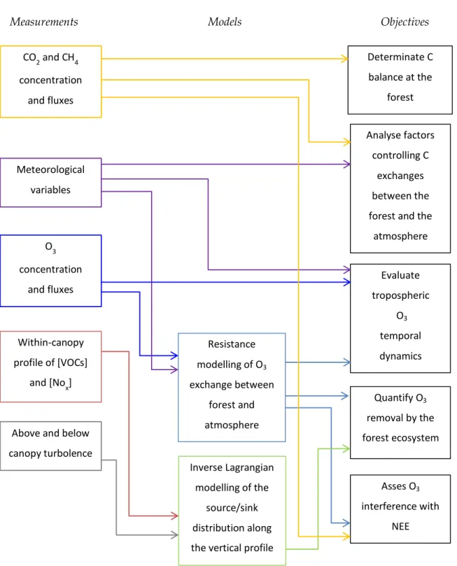
The main objectives of the PhD work were to (1) determinate the carbon balance at the holm oak forest (2) analyse factors controlling C exchanges between the forest and the atmosphere (3) evaluate tropospheric O3 temporal dynamics over the forest (4) quantify O3 removal by the forest ecosystem and (5) assess O3 interference with NEE.

To meet these objectives, CO2, H2O, CH4, O3 exchanges were measured through the eddy covariance technique over a Mediterranean forest on the Tyrrhenian coast of central Italy, between 2012 and 2015. NOx concentrations were measured along a 5-level vertical gradient from soil to above canopy from July 2013 to February 2014. Two field campaigns, which were carried out in January 2014 and in August 2015, were designed to measure VOCs concentrations distribution within the canopy and VOCs exchanges above the canopy. Measured data were combined with models in order to (1) infer the source/sink contribution of canopy layers to VOCs and NOx exchanges and to (2) quantify the individual contribution of O3 exchange pathways. The two respective models used were: (1) the Inverse Lagrangian modelling of the vertical gas source/sink distribution and (2) the Resistance modelling of O3 fluxes.

The following diagram (fig 1.2) shows the thesis work and outlines how measurements and modelling aided to meet the objectives.

Figure 1.2: Diagram of the PhD work activities (measurements and modelling), and their relations with the thesis objectives.

Objectives Measurements Models CO₂ and CH₄ concentration and fluxes O₃ concentration and fluxes Within-canopy profile of [VOCs] and [No_x] Meteorological variables

Above and below canopy turbolence Determinate C balance at the forest Analyse factors controlling C exchanges between the forest and the

atmosphere Evaluate tropospheric O3 temporal dynamics Quantify O3 removal by the forest ecosystem Asses O3 interference with NEE Resistance modelling of O3 exchange between forest and atmosphere Inverse Lagrangian modelling of the source/sink distribution along the vertical profile

2

Methods

Understanding of forest-atmosphere interactions has grown in the last decades, mainly due to the improvement of gas sensing technology and micrometeorological techniques.

In this chapter, measurements and data analysis methods are explained in details.

2.1

The study site

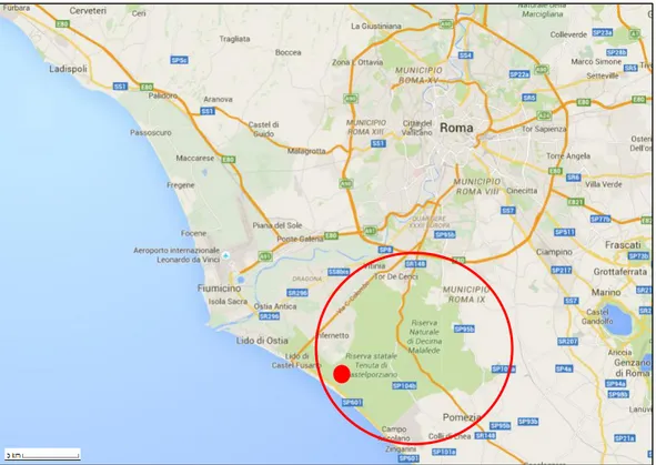
The presidential estate of Castelporziano is an hotspot for biodiversity in the Mediterranean, which hosted more than 1000 plants species (Davison et al., 2009). It is a protected area of about 4800 ha, of which 85% are forests. It is located on the coast of the Tyrrhenian sea, 25 km from Rome downtown. Castelporziano is included in the Long Term Ecosystem Research network (LTER – Italy).

Figure 2.1 Study site location, the red line surrounds the Castelporziano estate, the red dot indicates where the study forest is located.

The PhD research was carried out in a wild coastal rear dune ecosystem within the estate, 1.5 km from the seashore (41°70’42’’N, 12°35’72’’E - fig. 2.1), covered almost prevalently by an even-aged evergreen holm oak forest (Quercus ilex L.). Canopy mean height is 14 m and its structure is homogeneous with a leaf area index of 3.69 m2 _{leaf m}-2 _{ground. The understory} vegetation is poorly developed and formed prevalently by small shrubs of mock privet (Phillyrea latifolia L.).

Soil has a flat topography, with a sandy texture, and low water-holding capacity. The main soil physic-chemical properties are as follows: 33 g kg-1 _{clay, 116 g kg}-1 _{silt and, 851 g kg}-1 sand; pH in H2O is 6.85; total organic C, 8.73 g kg-1, total N, 0.56 g kg-1; C/N ratio 13.74 (Pinzari et al., 1999; Biondi et al., 2001).

Climate is typically Mediterranean: seasonality is pronounced, Summer periods are hot and dry, winters are moderately cold. Precipitation occurs prevalently during Spring and

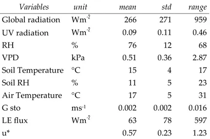
Autumn. Mean annual precipitation, averaged over 1999-2010, were 789.3 ± 230.6 mm y-1 _and mean monthly temperatures, averaged over the same period, range between 7.3 °C and 23.3 °C. Average, standard deviation and range of different environmental parameters measured during the study period are summarized in table 1.

Variables unit mean std range

Global radiation Wm-2 266 271 959 UV radiation Wm-2 0.09 0.11 0.46 RH % 76 12 68 VPD kPa 0.51 0.36 2.87 Soil Temperature °C 15 4 17 Soil RH % 11 5 23 Air Temperature °C 17 5 31 G sto ms-1 _{0.002 0.002 0.016} LE flux Wm-2 63 78 597 u* 0.57 0.23 1.23

Wind circulation followed a sea-land breeze regime, the dominant wind direction is S-SW during the morning and N-NE during the afternoon.

Due to its location, the forest is exposed to pollutants linked to both urban and rural activities, making the forest an ideal site for testing the pollution-vegetation interactions.

2.2

Micrometeorological methods

Micrometeorology is a branch of meteorology that studies small-scale atmospheric

phenomena, which occur within the planetary boundary layer (PLB). PLB is the part of the troposphere that is directly influenced by the interaction with the biosphere. There,

turbulence is influenced by shear stress and temperature profile. Shear stress can be express in velocity unit by the friction velocity (u*):

((

̅̅̅̅̅̅)

(

̅̅̅̅̅̅)

)

(8)

where ̅̅̅̅̅̅ and ̅̅̅̅̅̅ are the longitudinal and lateral momentum.

The thermic turbulence generated by temperature profile can be quantify by the Monin-Obukhov length (m):

( ⁄ )( ⁄ )

where k is the Von Karman constant (0.41), g is the gravitational acceleration (9.81 m s-2_{), T is} temperature in °K, H is the sensible heat flux (°K m-1 _s-1_{), ρa is the density of dry air (1.01 g m} -3_{) and cp is the specific heat capacity of air (1246 J kg}-1 _K-1_).

A dimensionless stability parameter (ζ) can be defined from L:

PLB above a rough surface, such a forest canopy, can be divided into the roughness sub-layer, which is a transition zone between the within canopy and the above canopy, the

inertial sub-layer, where is possible to infer fluxes through micrometeorological technique, and the Ekman sub-layer, which is the upper part of the PBL (Garratt, 1994).

Further, the micrometeorological methods used in this work to measure and model gas exchanges above, within and below the forest canopy are listed.

2.2.1 Eddy covariance technique for flux measurements

Eddy covariance (EC) technique allows to directly measure an average vertical flux at a single height. EC technique integrates fluxes over a large area and is representative of the whole ecosystem.

Following this technique, any measured scalar (x) or wind component (u, v or w) is

discomposed into its time-average component ( ̅) and its instantaneous deviation from the mean (x’). The vertical flux is calculated as the covariance of x’ and vertical wind velocity:

̅̅̅̅̅

assuming that the w time-average is equal to 0. Positive fluxes indicate gas release to the atmosphere while negative fluxes indicate uptake from the atmosphere.

The time-averaging is often set to 30 min, which is an adequate interval to include fluctuation contributing to the flux avoiding the occurrence of change in atmospheric conditions. Sensors measuring x and w must be sufficiently fast to include the higher frequency contributing to the flux, which depends on the eddy size, function of the

roughness length (z0) and measurements height (z). Data acquisition rate can vary between

few Hz and 30 Hz.

In order to obtain reliable measurements, quality assurances are required. In this work, the following procedure was applied:

Before calculation of the covariance, raw high frequency concentrations were filtered to remove spikes, identified as values exceeding 6 times the standard deviation calculated on a 1-minute window. Webb-Pearman-Leuning correction was applied to correct for air density fluctuation (WPL correction, Webb et al., 1980).

A double coordinate rotation procedure was performed to align the horizontal component of the wind (u) so that the means of lateral (v) and vertical (w) components were zero on each block of half-hour data, angle of attack was corrected following the procedure proposed by Nakai and Shimoyama (2012). Sonic temperature was corrected for the wind velocity fluctuations (Schotanus, 1983). After that, sonic anemometer and gas concentration signals were synchronized shifting the time series to maximize the covariance between them. Half-hourly fluxes were discarded when steady state condition were not fulfilled, following the test proposed by Foken and Wichura (1996).

u* was used as a criterion to ensure well developed turbulence. u* thresholds were

calculated for each year of measurement using u* and NEE nighttime data as described by Aubinet et al. (2012). Selected thresholds were 0.13 for 2012, 0.15 for 2013 and 2014, 0.16 for 2015. Data recorded during weak mixing condition (u* < u* threshold) were excluded from the analysis.

The contribution of the forest area around the tower to the EC measurements (fetch area) was evaluated according to Hsieh et al. (2000). Peak distance from measuring point to the maximum contributing source area outreached 80 m and 2 km up-wind from the tower during unstable and stable conditions, respectively. Data recorded when fetch area included cover types other than forest (peak distance from the measuring point to the maximum contributing source area > 400 m) were discarded.

Instrument detection limit was estimate for each half-hour as the root mean squared error of the covariance from zero in a range of ±30 - ±90 seconds away from the real lag, where it can be assumed that the w and x are no longer correlated (Langford et al., 2015). Half-hour fluxes below corresponding detection limit were considered not significantly different from zero. A detailed explanation of the EC technique and quality assurance methods can be found in Foken (2008) and Aubinet et al.(2012).

2.2.2 Inverse Lagrangian technique to evaluate source / sink distribution within the forest

canopy

The inverse Lagrangian technique (ILT) allows to derive the vertical source / sink

distribution of a gas within the canopy from the turbulence structure inside the canopy and the concentration of the gas measured along a vertical profile.

It is based on the “localized near field theory” (Raupach, 1989). The model assumes a relation between the source (or sink) magnitude associated to a layer (S) and the gas concentration measured in the same layer (X). This relation is made explicit by a dispersion matrix (D) that accounts for the concentration contribution due to the gas diffusion within the canopy, determinates by turbulent transport of the order of the canopy height (hc) or larger (far-field effect), and the gas persistence inside the canopy (near-field effect), which in turn depends on

eddies smaller that hc. The near field effect dominates if the travel time of a gas is small than

the Lagrangian time scale (TL), where

TL = 0.3 hc u*

The relation can be express as:

̃

where ̃ represents a concentration offset that is independent from S, and

Given the above, the far-field contribution can be expressed as:

(

) ∫

(15) where Fx(z) is the gas vertical flux at height z:

( )

∫ ( )

where Fg is the ground flux (at z=0) KH is the diffusion coefficient:

where σw is the standard deviation of the vertical wind component.

The far field effect dominates if the travel time of a gas is larger than TL, so that:

∫

[

(

)

(

)]

How presented integrals may be turned into finite sums can be found in Nemitz et al. (2000).

2.2.3 Resistance modelling of O

deposition

A common model to represent O3 uptake processes is the resistance analogy, where the individual strength of a sink is quantified using a resistance scheme (fig 2.2). First proposed by Hicks et al. (1987), the model consider a sink flux proportional to the difference in gas concentration between two locations, divided by the transfer resistance.

Gas deposition velocity (Vd) is computed in analogy to Ohm's law in electrical circuits:

Below, a brief description of the different resistances and their calculation.

Aerodynamic resistance

The aerodynamic resistance (Ra) describes the turbulent transport between z and z0. Ra can be estimated as (Garland, 1977):

( )

(20)

where ΨH and ΨM are stability correction for heat and momentum respectively, they are function of ζ and can be calculated as follow (Paulson, 1970):

Figure 2.2 Resistance deposition model for O3, from Wesely and Hicks (2000). Cz is the concentration at height z; C0 is the concentration at z0, Cc is the canopy concentration, Ra is the aerodynamic resistance at height z, Rb is the canopy boundary layer resistance, Rs is the stomatal resistance, Rct is the cuticular resistance, Rm is the mesophill resistance, Rg is the ground resistance, Rc is the total canopy resistance, which would replace the right side of the scheme.

for stable conditions ( ):

( )

( )

⁄

for unstable conditions ( ):

( ) (

) (

)

_{( )}

( ) (

)

where ( ) ⁄ (24)

Canopy Boundary layer resistance

The canopy boundary layer resistance (Rb) describes the transport trough the quasi-laminar

sub-layer (Owen and Thomson, 1963) and depends on the molecular diffusivity of the gas (Dx).

(

)

where B is the Stanton number that can be calculated after Garland (1977):

where Re is the Reynold number (

z

u*/v

Schmidt number (

v

/D

Canopy resistance

Considering the gas uptake process happen at a unique height (z0), the canopy resistance (Rc)

is calculated as the difference between Ra+Rb and the total resistance:

where Χ is the gas concentration and Fx is the measured flux. Thus, Rc is inferred by

measurements. Rc includes all the resistances for deposition on all canopy elements (stomata,

Stomatal resistance

If transpiration is the only source of water-vapour from the canopy surface, stomatal resistance to water vapour (Rs) can be estimated by EC measured evapotranspiration using

the evaporative/resistance method (Thom, 1975): ( ( ))

(28)

where qa is vapour pressure at z-d (kg kg−1), qs is the saturation mass fraction of H2O at air temperature (kg kg−1_{), γ is the psychrometric constant (4.08 ×10}−4 _K−1_{), λ is the vaporisation} heat for H2O (2.5 × 106 J kg−1), E is the measured latent heat flux (kg m−2 s−1).

This algorithm is based on the assumption that the gas diffusion inside the stomata is completely drive by Fick’s law, i.e. molecular diffusion. The small dimension of stomata prevent gas turbulent motion, justifying this assumption (Gerosa et al., 2007).

In this work, Rs was used to calculate stomatal conductance to O3 (GO3 ), calculated as the

inverse of Rs , multiplied for 0.61, which is the difference in diffusivity between O3 and H2O (Massman, 1998). GO3 was multiplied to O3 concentration at the canopy level to calculate the O3 stomatal flux. O3 concentration at the canopy level was calculated as:

(29)

where RbO3 is the boundary layer resistance to O3.

Soil resistance

Soil resistance includes in-canopy aerodynamic resistance (Rac) and ground resistance (Rg). Rac depends on hc and LAI, its formulation after Erisman et al. (1994) is:

(30)

Rg depends on soil water content (swc, %) and is calculated following Zhang et al. (2002) as:

where Rg1 and Rg2 are constant resistances (200 and 300 s m−1, respectively), swc10 is the swc

measured at 10 cm depth, swcfc is the swc at field capacity (28 %), calculated as the maximum

value of swc10 after precipitation events (Fares et al., 2014).

Rg was used to calculate the soil O3 deposition fraction, multiplying the inverse of Rg for the

O3 concentration measured at the soil level.

Cuticular resistance

Cuticular resistance (Rct) depends on the leaf wetness and is calculates following Zhang et al.

(2002), assuming that the gas concentration just above the cuticles is negligible.

( ) ( ) ⁄ (32)

( ) ( ) ⁄ (33)

where Rct(dry)0 and Rct(wet)0 are constant values (6000 and 400 s m−1, respectively) suggested by

Zhang et al. (2002) and RH is the relative humidity of air (%). Wet condition are assumed when RH > 60%(Fares et al., 2014). Rct was used to calculate the cuticles O3 deposition fraction, multiplying the inverse of Rct for the O3 concentration at the canopy level.

2.2.4 Measurements and instrument set-up

Meteorological variables were measured at 1-minute resolution in proximity of the canopy level (15 m), onto a 20 m high tower. The instrumentation included a Davis vantage pro meteorological station (Davis Instruments Corp. CA, USA) used to monitoring relative humidity (RH, %), air temperature (T air, °C), global solar radiation (rad, Wm-2_{), UV radiation} (280-360 nm, UV, Wm-2_{) and precipitation (prec, mm). Instantaneous three-dimensional wind} velocity (u, v, w, ms-1_{) and direction (winddir, °) were measured with a sonic anemometer} (Windmaster 3d Anemometer, Gill Instruments Limited, UK). Photosynthetic photon flux density was measured with a LI-190 Quantum sensor (LI- COR, Licoln, NE, USA), soil humidity (RHsoil, %) and temperature (T soil, °C) were measured by a Vaisala 102 HUMICAP

180 capacitive relative humidity sensor (HMP45C, Campbell Scientific) at a single point (10, 50, 100 cm depth) inside of the flux footprint. Data collection was performed by a datalogger (CR3000, Campbell Scientific, Shepshed, UK).

O3 concentrations were measured using a UV photometric O3 analyser (49i, Thermo Scientific), with a precision of 0.5 ppb.

NO and NO2 concentrations were measured by a chemiluminsescent analyser (42i, Thermo Scientific), with a precision of 0.4 ppb.

VOCs were measured with a proton-transfer-reaction mass-spectrometer (PTR-MS, Ionicon Analytik GmbH) which was located in an air-conditioned cabinet next to the tower. During measurements, gas standards were measured every 24 hour to calibrate the instrument.. 23 compounds were measured, between them: isoprene, monoterpenes, and their oxidation products (BVOCs), methanol, acetaldehyde, acetone (OVOCs) acetonitrile, benzene, hexenal, toluene and xylenes origin (AVOCs).

O3, NOx and VOC were sampled through a 5-level vertical profile. Measurement heights were 19.7 m (above canopy), 14.9 m (canopy level), 12 m , 7 m (within the canopy) and 2.4 m (below canopy). Air was sampled using separate sampling lines (20-m long Teflon tubes, with 4-mm inner diameter) through which air flowed continuously to avoid any memory or surface effects. To avoid contamination and flow problems, Teflon filters (PFA holder, PTFE membrane, 2 μm pore size) were installed at the sampling inlets and replaced every two weeks. A custom- made valve system sampled ozone sequentially for 6 min at each

measuring height. Data collection and sampling system control were performed using a data logger (CR3000, Campbell Scientific, Shepshed, UK).

Concentrations measurements for fluxes calculation were performed at 10 Hz. Air was sampled continuously at 19.7 m height near the sonic anemometer.

CO2 and H2O concentrations were measured by a closed path infrared analyser (LI-7200, Li-Cor, Inc., Nebraska, USA), CH4 concentration was measured by an open path gas analyser (LI-7700, Li-Cor, Inc., Nebraska, USA).

O3 measurements were made by chemiluminescence using coumarin dye with a custom-made instrument developed by the National Oceanic and Atmospheric Administration (NOAA, Silver Spring, MD, Bauer and Hultman, 2000). The chemiluminescence signal was calibrated against 30-min average O3 concentrations from the UV O3 monitor.

10 Hz data were stored in a datalogger (LI- 7550, Li-Cor, Inc., Nebraska, USA), divided into half-hour files.

An additional EC tower, 2.4 m height, were placed below the canopy. There, O3 measurements were performed using a dry chemiluminescence Rapid Ozone Flux Instrument (ROFI Mk2; Muller et al., 2009), H2O and CO2 were measured by a close path infrared gas analyser (LI-7000, Li-Cor, Inc., Nebraska, USA) and wind velocity were measured using a sonic anemometer (RM Young 81000, RM Young Company, Michigan, USA). Measurements were logged at 10 Hz into a datalogger (CR 3000, Campbell Scientific, Shepshed, UK).

2.3

Statistics

Kolmogorov-Smirnov test (KS test) was used to test normality for all considered variables. According to the test results, parametric or non-parametric statistics were chosen. One-way ANOVA (parametric) or Kruskal-Wallis (non-parametric) tests were used to compare means. When differences were found, a post-hoc test was performed in order to evaluate which group differs from others.

2.3.1 Multiple Linear Regression

The attempt of multiple liner regression (Pearson and Lee, 1908) is to infer the relationship between several independent continuous variables (predictors) and a dependent variable. This relationship is represented as a linear equation:

where y is the dependent variable, x1…n are the predictors, β1…n are the coefficients associated to each predictor and ε is the intercept. β is the expected change of y for unit change of x, ε is the prediction of the model if all x values were set to zero.

In this work, multiple regression was used to develop two empirical models to gap-fill forest soil level H2O and O3 fluxes. Dataset was split into two subset. Randomly selected 70% of the dataset was used to build the models and then cross-validated with the remaining 30% of the data (chapter 4).

Different predictor values were tested trough step-wise regression, which was used to

extract the best subset of predictor variables for use in the forecasting models. This technique successively adds or removes variables based on the t-statistics of their estimated

coefficients. This coefficients where estimated using the least square approach, i.e., setting coefficients and intercept equal to the values that minimize the sum of squared errors within the sample of data to which the model is fitted.

Predictor variables tested by step-wise regression were: soil humidity and soil temperature measured at 10, 50, 100 cm depth, friction velocity above canopy and at soil level, air

temperature above canopy and at soil level, above canopy H2O fluxes (just for soil level H2O flux modelling) above canopy O3 fluxes (just for soil level O3 flux modelling)

Multiple linear regression technique is subjects to a series of assumptions: predictor variables are assumed to be error-free, that is, not contaminated with measurement errors (weak

exogeneity), the relation between the dependent variable and predictor should be linear

(linearity), predictors must have the same variance in their errors, regardless of the values of the predictor variables (homoscedasticity), errors must be randomly distributed (independence

of errors) and predictor must not be highly correlated each other (lack of multicollinearity). The

latter assumption was not fulfilled, this can make some variables statistically insignificant when they should be significant, so that the model was not use to infer functional

relationships between predictors and dependent variables, but just to fill data gaps, when present.

2.3.2 Partial Least Squared Regression

Partial Least Square (PLS) regression is a multivariate technique that combines features from principal component analysis (PCA) and multiple linear regression, and is useful when predictors are highly correlated or even collinear. PLS generates linear combinations of the original predictors (components), which best explain the variance among parameters and maximize covariance between predictors and the dependent variable. These new

components, generate from both predictors and dependent variables, are no longer correlated and became the new predictors variables.

The contribution of the original variables to each components can be inferred by the associated weight. The weights interpretation is easy since the sum of the square of the weight within the component yields to 1. This property allows the partition of the variance explained by the model between the original variables.

Before performing the analysis datasets must be centered to have mean 0 and scaled to have standard deviation 1, to avoid scale influence on results. Number of components used by the model is chosen as the number of components which performed lower mean square error, calculated using k-fold cross-validation. This procedure divides dataset into k disjoint subsamples, chosen randomly but with roughly equal size, avoiding model overfitting. In this work, PLS regression was used to infer functional relationships between

environmental parameters and CH4 flux measured above canopy (chapter 3) and to explore the interactions between stomatal O3 uptake with NEE (chapter 4).

2.3.3 Singulars Spectrum Analysis

Singular Spectrum Analysis (SSA) is a non-parametric technique that decomposes a time series into a set of additive components, which are (i) a trend, (ii) a set of periodic series and (iii) a random noise (Golyandina et al., 2001). The sum of these components is the original time series. SSA results depends on the windows length chosen for the analysis.

SSA consists of two complementary stages: decomposition and reconstruction. Both stages include two separate steps, which are the follows:

Step 1. Embedding

Let Y being a time series of length n, L the window length, an integer with 2 < L < N. The first step transfers the one-dimensional time series Y into the multi-dimensional series X (trajectory matrix). Columns of X represent all the possible position of the window L, so that K = n – L + 1 is the number of columns. X is a Hankel matrix, i.e. all elements along the diagonal are equal.

Step 2. Singular values decomposition of the trajectory matrix:

The second step computes the eigenvalues and eigenvectors of the matrix X, which is decomposed in d-rank one elementary matrix where d is the number of non-zero eigenvalues in decreasing order.

Step 3. Reconstruction:

In the third step, each matrix obtained by the step 2 is transformed through averaging over the diagonals (Hankelization).

Step 4. Grouping:

The last step reconstructs a one-dimension matrix, expresses as the sum of the trajectory matrices corresponding to each partition.

A detailed description of the SSA algorithms can be found in Golyandina et al. (2001) The principal advantage of SSA with respect to other decomposition algorithms is that is not necessary to make any statistical assumptions such as stationarity of the series or normality of the residuals.

In this work, SSA was used to extract the sinusoid series corresponding to the daily dynamic from the environmental parameters time series (chapter 5). This was done because most of the environmental parameters are completely driven by the daily course, which makes them mutually correlated.

2.3.4 Feed Forward Back-Propagation Artificial Neural Network

Artificial Neural Network (ANN) were initially developed with the intent of create an artificial system to reproduce mammalian brain (Olden et al., 2004). Can be defined as a parallel processor composed by simple processing elements (neurons) connected by communication channels, with the capacity of storing knowledge (Papale and Valentini, 2003). Each neuron have small amount of local memory and works on the input they received via communication channels.

ANNs are very powerful in analysing and modelling non-linear relationships because of their capacity of learn from examples and generalize.

A training dataset composed by input and the relative output is necessary to adjust neurons weight and connections. It is important to scale the dataset, i.e. between 0 and 1, to avoid any scale influence on results. In this work, ANNs were trained by feed forward

back-propagation algorithm (Rumelhart, 1986): information flows unidirectionally trough the network and the errors ANN makes using the training set to model the output are used to adjust neurons weight and connections strength. Datasets is split randomly into three subset, training, test and validation sets. Training subset is used to compute the weights of the network’s neurons, the test subset for stopping the training process checking the model generalization ability. Last subset is used to validate the model.

ANNs were organized in three layer: an input layer, an hidden layer and an output layer (fig. 2.3). The optimal number of neurons in the hidden layer was determined by comparing the performance of different cross-validated networks, with 1 – 4 hidden neurons, and choose the number that produced better network performance.

Figure 2.3 Example of an ANN structure. Input layer is composed by 5 neurons, hidden layer by 3 neurons and the output layer by 1 neuron. w is the neuron weight, b is the bias.

Once the network in trained, weights and connections are established and ANN can simulate the output when input are provided. Each input is multiplied by the respective weight assigned to its connections and arrives to the neuron in the hidden layer. There, this

information is summed with the other arriving from the other input, and transformed by an activation function. Information is then transferred to the output layer, where again it is multiplied by connection weights and transformed by the activation function, to be converted into the final result (output).

ANNs are often treated as “black box” because is not possible to extrapolate equations which explain the mechanisms that occur within the network. However, some algorithms have been proposed to overcome this issue, and the relative importance of each input variable can be evaluated. Gevrey et al. (2003) and Olden et al. (2004) provide a comparison of the different methods for estimating variables importance in ANN applications, in this work, three of the existing methods were applied:

Partial derivatives method (Dimopoulos et al., 1995) :

This method produced a profile of the output variations for changes of each input variable. The link between the variation of the output and the modification of the input is the partial derivative of each activation function with respect to its input.

Given an ANN with ni inputs, one hidden layer with nj neurons and one output, where

logistic sigmoid function is used for activation, the partial derivatives of the output with respect to one input are (Gevrey et al., 2003):

∑

(

)

where Sj is the derivative of the output with respect to its input, Ihj is the response of the h

hidden neuron, who is the weight between the output neuron and the h hidden neuron, wih is

the weight between the h hidden neuron and the i input neuron.

The advantage of this technique is that a profile of each input variable can be analysed without altering its magnitude, that is without producing artefacts. The weakness of this technique is that it provides information on one input at time and does not show the interaction between inputs (Gevrey et al., 2006).

Connection weights approach (Olden and Jackson, 2002):

This method splits the connection weights (hidden layer and output layer) into components associated with each input neuron and sums the products across all the layer to establish importance ranks.

∑

where who is the weight between the output neuron and the h hidden neuron, wih is the weight

between the h hidden neuron and the i input neuron.

This algorithm was recognized to have the best ability to correctly identify input importance in neural networks by Olden et al. (2004), which compared the existing algorithms using Monte Carlo simulations, i.e. using data with known numeric relationships.

Perturb method (Gevrey et al., 2003):

This method is a sensitivity analysis that assesses the effect of small changes in one input on the network’s output. One of the input is increased in steps of 10% up to 50% of the original value, while keeping all the others input unchanged.