BERNSTEIN-TYPE APPROXIMATION USING THE BETA-BINOMIAL DISTRIBUTION Andrea Pallini
1. INTRODUCTION
The Bernstein polynomials are generally regarded as the most basic tools for the uniform approximation in the sense of Weierstrass of a continuous and real-valued function g on the closed interval [0,1]. The Bernstein polynomials are elegant linear positive operators. The Bernstein polynomials of order m are de-fined by the binomial distribution p k t , for m( ; ) k=0,1, ,… m, where t ∈[0,1] is the domain of g . The convergence of the Bernstein polynomials to g is uni-form, as m → ∞ . Multivariate versions of the Bernstein polynomials can be de-fined by products of independent binomial distributions. See Korovkin (1960), chapter 1, Davis (1963), chapter 7, Feller (1968), chapter 6, Feller (1971), chapter 7, Rivlin (1981), chapter 1, Cheney (1982), chapters 1 to 4, Lorentz (1986), DeVore and Lorentz (1993), chapter 10, Phillips (2003), chapter 7.
The Bernstein-type approximations of order m in Pallini (2005) consider a convenient approximation coefficient in linear kernels and improve on the degree of approximation of the Bernstein polynomials. The convergence of these Bern-stein-type approximations is uniform, as m → ∞ .
Here, following Pallini (2005), we study the Bernstein-type approximation of order m that can be defined by using the beta-binomial distribution. We obtain integral operators that approximate to a continuous and real-valued function g on any closed interval D⊆R1. We also obtain their multivariate versions for a
continuous and real-valued function g on any closed interval D⊆Rq. The
con-vergence of these Bernstein-type approximations is uniform, as m → ∞ .
In section 2, we overview the univariate and the multivariate Bernstein poly-nomials. In section 3, we present some basic notions for the use of the beta-binomial distribution in approximation. In section 4, we propose the univariate and multivariate Bernstein-type approximations that can be obtained by the beta-binomial distribution. We study the uniform convergence and the degree of ap-proximation. We also compare these Bernstein-type approximations with the Bernstein polynomials. In section 5, we study the Bernstein-type estimators for
smooth functions of the population means. In section 6, we discuss the results of a simulation study on some examples of smooth functions of means. Finally, in section 7, we conclude the contribution with comments and remarks.
We refer to Barndorff-Nielsen and Cox (1989), chapter 4, and Sen and Singer (1993), chapter 3, for more details on the smooth functions of means and their application to classical inferential problems.
2. BERNSTEIN POLYNOMIALS
Let g be a bounded and real-valued function defined on the closed interval [0,1]. The Bernstein polynomial B g x of order m( ; ) m for the function g is de-fined as 1 0 ( ; ) m ( ) k(1 )m k m k m B g x g m k x x k − − = ⎛ ⎞ = ⎜ ⎟ − ⎝ ⎠
∑
, (1)where m is a positive integer number, and x ∈[0,1]. If ( )g x is continuous on [0,1]
x ∈ , then we have that B g xm( ; )→g x( ), as m → ∞ , uniformly, at any point x ∈[0,1].
Let g be a bounded and realvalued function defined on the closed q -dimensional cube [0,1]q. We let
1
x ( , , )T
q
x x
= … , where x [0,1]∈ q. The
multi-variate Bernstein polynomial B gm( ; x) for the function g is defined as
1 1 1 1 m 1 1 0 0 ( ; ) ( , , ) q q m m q q k k B g x g m v− m v− = = =
∑ ∑
… 1 1 1 1 1 1 1 (1 ) q(1 ) q q q v m v v m v q q q m m x x x x v v − − ⎛ ⎞ ⎛ ⎞ ⋅⎜ ⎟ ⎜ ⎟ − − ⎝ ⎠ ⎝ ⎠ , (2) where m ( , ,1 )T q m m= … are positive integer numbers, and x [0,1]∈ q. The
multi-variate Bernstein polynomial B gm( ; x) is of order m , where
1 q i i m m = =
∑
, andx [0,1]∈ q. The multivariate Bernstein polynomial ( ; ) m
B g x converges to (x)g uniformly, at any q -dimensional point of continuity x [0,1]∈ q, as
i m → ∞ , where i= … . 1, ,q
3. THE BETA-BINOMIAL DISTRIBUTION
More accurate versions of the Bernstein polynomials B g x and m( ; ) B gm( ; x), defined by (1) and (2), where x ∈[0,1] and x [0,1]∈ q, can be obtained by the
beta-binomial distribution, that is reviewed and studied in Wilcox (1981) and Johnson, Kemp and Kotz (2005), chapter 6.
The standard beta distribution ( ; , )p t a b , with parameters a > and 0 b > , 0 has probability density function (p.d.f.) p t a b( ; , ) { ( , )}= B a b −1ta−1(1−t)b−1, for
every (0,1)t ∈ . We also recall that 1 1 1
0 ( , ) a (1 )b B a b =
∫
t − −t − dt, where 1 ( , ) ( ( )) ( ) ( ) B a b = Γ a b+ − Γ a Γb , and 1 0 ( )a ∞t e dta− −tΓ =
∫
. See Balakrishnan andNevzorov (2003), chapters 16 and 20.
The beta-binomial random variable (r.v.) Y , with parameters m , 0a > and 0
b > , has p.d.f. p k a bm( ; , ) Pr[= Y k= , that is defined as ]
1 1 1 1 0 ( ; , ) { ( , )} a k (1 )b m k m m p k a b B a b t t dt k − + − + − − ⎛ ⎞ =⎜ ⎟ − ⎝ ⎠
∫
, (3)for every k=0,1, ,… m. We can rewrite the definition (3) as
1 1 1 1 0 ( ; , ) { ( , )} ( ; ) a (1 )b m m p k a b = B a b −
∫
p k t t − −t − dt, where ( ; ) k(1 )m k m m p k t t t k − ⎛ ⎞ =⎜ ⎟ −⎝ ⎠ is the binomial p.d.f., with parameters m and t , [0,1]t ∈ , for every k=0,1, ,… m. Moments of the beta-binomial r.v. Y , are obtained by integrating the moments of the binomial p.d.f. p k t , m( ; ) t ∈[0,1],
0,1, ,
k= … m, that are functions of t , t ∈[0,1], through the definition (3) of the beta-binomial p.d.f. p k a b , m( ; , ) k=0,1, ,… m.
In particular, the first two moments about the origin, ' ' 1( , )a b 1
λ ≡ and λ
' '
2( , )a b 2
λ ≡ , of the beta p.d.f. ( ; , )λ p t a b , with values t ∈[0,1], are
' 1 1( , ) (a b a b a) λ = + − , (4) ' 1 2( , ) {(a b a b a b)( 1)} (a a 1) λ = + + + − + , (5)
and the third moment about the origin ' 3
λ is
' 1
3 {(a b a b)( 1)(a b 2)} (a a 1)(a 2)
See Balakrishnan and Nevzorov (2003), chapters 5 and 16, and Johnson, Kemp and Kotz (2005), chapter 3.
The values of the parameters a and b , in the moments ' 1( , )a b
λ and '
2( , )a b
λ , given by (4) and (5), respectively, of the beta p.d.f. ( ; , )p t a b , with values
(0,1)
t ∈ , that yield a conveniently small quantity
1
' '
1( , )a b 2( , ) {(a b a b a b)( 1)} ab
λ −λ = + + + − , (7)
can be regarded as constructive. More precisely, constructive values of a and b in (7) can directly help to improve the numerical performance of the Bernstein-type approximations that we are going to introduce in section 4. Constructive values of a and b in (7) can lower their uniform convergence rates, as m → ∞ .
The quantity ' '
1( , )a b 2( , )a b
λ −λ given by (7) does not admit a minimizer, for 0
a > and b > . For further details and descriptions, see sections 6 and 7. 0 4. BERNSTEIN-TYPE APPROXIMATIONS
4.1. Bernstein-type approximations
Let g be a bounded and real-valued function defined on the closed interval
1
D⊆R . The Bernstein-type approximation ( )s ( ; , , ) m
C g x a b of order m for the function ( )g x is defined as
{
}
1 1 ( ) 1 0 0 ( ; , , ) ( , ) m ( ( ) ) s s m k C g x a b B a b − g m− m k t− x = =∫
∑
− + 1(1 ) 1 a k b m k m t t dt k + − + − − ⎛ ⎞ ⋅⎜ ⎟ − ⎝ ⎠ , (8)where s > −1/2 is fixed, m is a positive integer number, and x D∈ . Properties of the Bernstein-type approximations ( )s ( ; , , )
m
C g x a b , given by (8), x D∈ , are outlined in Appendix 8.1.
If the function ( )g x is continuous on x D∈ , where s > −1/2, then
( )s ( ; , , ) ( ) m
C g x a b →g x , as m → ∞ , uniformly at any point x D∈ . In Appendix 8.2, we provide a proof of this uniform convergence.
Let g be a bounded and real-valued function defined on the closed interval D⊆Rq. The Bernstein-type approximation ( )
ms ( ; x, , )
C g a b of order m for the function (x)g is defined as
1 1 1 1 1 1 1 1 1 1 ( ) m 0 0 0 0 1 ( ) ( ; x, , ) { ( , )} ( ) q q s m m s q k k s q q q q q m m k t x C g a b B a b g m m k t x − − − = = − − ⎛ − + ⎞ ⎜ ⎟ = ⎜ ⎟ ⎜ ⎟ ⎜ − + ⎟ ⎝ ⎠
∑ ∑
∫ ∫
1 1 1 1 1 1 1 1 1 (1 ) q a k b m k q m m t t k k + − + − − ⎛ ⎞ ⎛ ⎞ ⋅⎜ ⎟ ⎜ ⎟ − ⎝ ⎠ ⎝ ⎠ 1 1 1 (1 ) q q q a k m b k q q q t + − −t + − − dt dt , (9)where 1/2s > − is fixed, m ( , ,= m1… mq)T are positive integer numbers, 1 q i i m m =
=
∑
, and x D∈ . Properties of the Bernstein-type approximations( )
ms ( ; x, , )
C g a b , given by (9), x D∈ , are outlined in Appendix 8.1.
If the function (x)g is continuous on x D∈ , where s > −1/ 2, then
( )
ms ( ; x, , ) (x)
C g a b → g , as m → ∞ , uniformly at any q -dimensional point x D∈ . In Appendix 8.2, we provide a proof of this uniform convergence.
4.2. Degrees of approximation
Let ( )ω δ be the modulus of continuity of the real-valued function g , for every 0δ > . The modulus of continuity ( )ω δ of the function ( )g x , where x D∈ , is defined as the maximum of g x( 0)−g x( ) , for x0−x < , where δ
0,
x x D∈ . If the function
g
is continuous, then ( )ω δ → , as 0 δ → . 0Setting δ =m−1/2, for every x D∈ , it can be shown that the Bernstein-type
approximation ( )s ( ; , , ) m
C g x a b , given by (8), has degree of approximation
( )s ( ; , , ) ( ) m C g x a b −g x 1 2 1 ' ' 1/2 1 2 [ 1 m m− − −s { ( , )λ a b λ ( , )}] (a b ω m− ) ≤ + − , (10)
where the quantity ' ' 1( , )a b 2( , )a b
λ −λ is given by (7). See Appendix 8.3. We let 1/2 2 1 |x| q i i x = ⎛ ⎞ = ⎜ ⎟
⎝
∑
⎠ , where x D∈ . The modulus of continuity ( )ω δ of the real-valued function (x)g , x D∈ , for every δ > , is defined as the maximum of 00
(x ) (x)
g −g , for |x -x|0 < , where δ x , x D0 ∈ . If the function g is continuous,
Setting δ =m−1/2, for every x D∈ , it can be shown that the multivariate
Bern-stein-type approximation C( )ms ( ; x, , )g a b , given by (9), has degree of
approxima-tion ( ) ms ( ; x, , ) (x) C g a b −g 1 2 1 ' ' 1/2 1 2 1 1 q s { ( , ) ( , )} ( ) i i m− m− − λ a b λ a b ω m− = ⎡ ⎛ ⎞ ⎤ ≤ ⎢ + ⎜ ⎟ − ⎥ ⎢ ⎝ ⎠ ⎥ ⎣
∑
⎦ , (11) where 1 q i i m m ==
∑
, and the quantity ' ' 1( , )a b 2( , )a bλ −λ is given by (7). See Appen-dix 8.3.
4.3. A comparison
For a convenient value of the approximation coefficient s , the Bernstein-type approximations ( )s ( ; , , )
m
C g x a b and ( )
ms ( ; x, , )
C g a b , given by (8) and (9), where 1/2
s > − , can typically outperform the Bernstein polynomials B g x and m( ; )
m( ; x)
B g , given by (1) and (2), for any function g to approximate, for every x D∈ and x D∈ , respectively.
Choosing a value of s , where s > −1/2, can only modify the coefficients in the degrees of approximation (10) and (11), without affecting their modulus of continuity ω(m−1/2), for any fixed
1 q i i m m =
=
∑
. Large values of s do not bring any advantage, with typical examples of application for the Bernstein-type ap-proximations Cm( )s ( ; , , )g x a b and Cm( )s ( ; x, , )g a b , defined by (8) and (9),respec-tively, where s > −1/2, x D∈ and x D∈ . The convergence to unity of the coef-ficients that distinguish the degrees of approximation (10) and (11) is rather fast, as s increases.
In Figure 1, we compare the Bernstein polynomial B g x , given by (1), with m( ; ) the Bernstein-type approximation ( )s ( ; , , )
m
C g x a b , given by (8), for the approxima-tion of the funcapproxima-tions g x( )=x3+x2+ , and x g x( )=x2+ , [0.25,0.75]x x ∈ ,
4
m = , 1.5a = , 10b = , s = −0.1, 0.005,0.05,0.5,1.5− . We also compare the Bernstein polynomial B gm( ; x), given by (2), with the Bernstein-type
approxima-tion ( )
ms ( ; x, , )
C g a b , given by (9), for the approximation of the function
1 2 1 (x) ( 1) ( 1) g = x + − x + , x ( ,= x x1 2)T, x ∈1 [0.25,0.75], x ∈2 [0.45,0.85], 1 2 4 m =m = , a =1.5, b =10, 0.1, 0.005,0.05,0.5,1.5s = − − . The values m =4
0.3 0.5 0.7 0.00 0.05 0.10 0.15 0.20 (i) 0.3 0.5 0.7 0.00 0.05 0.10 0.15 0.20 0.3 0.5 0.7 0.00 0.05 0.10 0.15 0.20 0.3 0.5 0.7 0.00 0.05 0.10 0.15 0.20 0.3 0.5 0.7 0.00 0.05 0.10 0.15 0.20 0.3 0.5 0.7 0.00 0.05 0.10 0.15 0.20 0.3 0.5 0.7 0.00 0.02 0.04 0.06 0.08 (ii) 0.3 0.5 0.7 0.00 0.02 0.04 0.06 0.08 0.3 0.5 0.7 0.00 0.02 0.04 0.06 0.08 0.3 0.5 0.7 0.00 0.02 0.04 0.06 0.08 0.3 0.5 0.7 0.00 0.02 0.04 0.06 0.08 0.3 0.5 0.7 0.00 0.02 0.04 0.06 0.08 0.3 0.5 0.7 0.00 0.01 0.02 0.03 0.04 (iii) 0.3 0.5 0.7 0.00 0.01 0.02 0.03 0.04 0.3 0.5 0.7 0.00 0.01 0.02 0.03 0.04 0.3 0.5 0.7 0.00 0.01 0.02 0.03 0.04 0.3 0.5 0.7 0.00 0.01 0.02 0.03 0.04 0.3 0.5 0.7 0.00 0.01 0.02 0.03 0.04
Figure 1 – Differences B g xm( ; )−g x( ), (hatched line), and Cm( )s( ; , , )g x a b −g x( ), (solid line), for
the smooth function g x( )=x3+x2+ , where x x ∈[0.25,0.75], where m =4, a =1.5, and
10
b = , with s = −0.1 (the worst performance), s = −0.005,0.05,0.5, and s =1.5 (the best per-formance) (panel (i)). Differences B g xm( ; )−g x( ), (hatched line), and Cm( )s( ; , , )g x a b −g x( ), (solid
line), for g x( )=x2+ , where x x ∈[0.25,0.75], where m =4, a =1.5 and b =10, with s = −0.1 (the worst performance), s = −0.005,0.05,0.5, and s =1.5 (the best performance) (panel (ii)). The difference B gm( ; x)−g(x), (hatched line), and Cm( )s( ; x, , )g a b −g(x), (solid line), for
1
2 1
(x) ( 1) ( 1)
g = x + − x + , where x ∈1 [0.25,0.75], x ∈2 [0.45,0.85], where m1=m2= , 4 a =1.5,
and b =10, with s = −0.1 (the worst performance), s = −0.005,0.05,0.5, and s =1.5 (the best performance) (panel (iii)).
and m1=m2 = are very small, computationally. In any case, the numerical per-4
formances of the Bernstein-type approximations ( )s ( ; , , ) m C g x a b , [0.25,0.75]x ∈ , and ( ) ms ( ; x, , ) C g a b , x ( ,= x x1 2)T, x ∈1 [0.25,0.75], x ∈2 [0.45,0.85], are always very effective.
5. ESTIMATION OF SMOOTH FUNCTIONS OF MEANS
5.1. Bernstein-type estimators
The Bernstein-type approximations ( )s ( ; , , ) m
C g x a b and (s)
m( ; x, , )
C g a b , given by (8) and (9), where x D∈ ⊆R1 and x D∈ ⊆Rq, can be used for estimating
smooth functions of the population means in the statistical inference on a ran-dom sample of n independent and identically distributed (i.i.d.) observations.
Let X be a univariate random variable with values x D∈ , distribution func-tion F , and finite mean µ=E X[ ]. We want to estimate a population character-istic ( )θ =g µ , where g is a smooth function g D: →R1. The natural estimator of θ is θˆ=g x( ), where 1 1 n j j x n− X =
=
∑
is the sample mean, calculated on a ran-dom sample of n i.i.d. observations Xj, 1, ,j = … , of X. An alternative estima-ntor of θ =g( )µ is the Bernstein-type estimator C( )ms ( ; , , )g x a b ,
1 ( ) 1 1 0 0 ( ; , , ) { ( , )} m ( ( ) ) s s m k C g x a b B a b − g m− m k t− x = =
∫
∑
− + 1(1 ) 1 a k b m k m t t dt k + − + − − ⎛ ⎞ ⋅⎜ ⎟ − ⎝ ⎠ , (12)where 1/2s > − is fixed. The Bernstein-type estimator (12) follows from the definition (8) of C( )ms ( ; , , )g x a b , 1/2s > − , by substituting x D∈ with the sample mean x , where x ranges in D .
Let X be a q -variate random variable with values x D∈ , where
1
X (= X , ,… Xq)T, with distribution function F , and finite q -variate mean [X]
E
µ= , µ=( , ,µ1… µq)T. We want to estimate θ=g( )µ , where g: D→R1.
Its natural estimator is θˆ=g( x ), where x ( , ,= x1… xq)T is the sample mean on a
random sample of n i.i.d. q -variate observations X , i i= … , of X , 1, ,n 1 1 n i ij j x n− X =
=
∑
, 1, ,i= … . An alternative estimator of q θ= g( )µ is the multi-variate Bernstein-type estimator C( )ms ( ; x, , )g a b ,1 1 1 1 1 1 1 1 1 1 ( ) m 0 0 0 0 1 ( ) ( ; x, , ) { ( , )} ( ) q q s m m s q k k s q q q q q m m k t x C g a b B a b g m m k t x − − − = = − − ⎛ − + ⎞ ⎜ ⎟ = ⎜ ⎟ ⎜ ⎟ ⎜ − + ⎟ ⎝ ⎠
∑ ∑
∫ ∫
1 1 1 1 1 1 1 1 1 (1 ) q a k b m k q m m t t k k + − + − − ⎛ ⎞ ⎛ ⎞ ⋅⎜ ⎟ ⎜ ⎟ − ⎝ ⎠ ⎝ ⎠ 1 1 1 (1 ) q q q a k b m k q q q t + − −t + − − dt dt , (13)where 1/2s > − is fixed. The multivariate Bernstein-type estimator (13) follows the definition (9) of Cm( )s ( ; x, , )g a b , s > −1/ 2, by substituting x D∈ with the
sample mean x , where x ranges in D .
5.2. Orders of error in probability of the Bernstein-type estimators
We know that ( 1/2)
p
x = +µ O n− , as n → ∞ . We also know that 1/2
( ) ( ) p( )
g x = g µ +O n− ,
as n → ∞ . It is shown that the Bernstein-type estimator ( )s ( ; , , ) m
C g x a b , given by (12), for s > −1/2, is a consistent estimator of ( )g µ , as m → ∞ and n → ∞ . In particular, it is shown that
( )s ( ; , , ) ( ) ( 2 1s ) ( 1/2)
m p
C g x a b = g µ +O m− − +O n− , (14)
for s > −1/ 2, as m → ∞ and n → ∞ . See Appendix 8.4.
We know that x= +µ O (p n−1/2), where xi =µi +O np( −1/2), 1, ,i= … , as q n → ∞ . We also know that
1/2
( x) ( ) p( )
g = g µ +O n− ,
as n → ∞ . It is shown that the multivariate Bernstein-type estimator
( )
ms ( ; x, , )
C g a b , given by (13), where m ( , ,= m1… mq)T, for s > −1/2, is a
consis-tent estimator of ( )g µ , as m → ∞i , i= … , and n → ∞ . In particular, it is 1, ,q
shown that ( ) 2 1 1/2 m 1 ( ; x, , ) ( ) ( ) ( ) q s s i p i C g a b g µ O m− − O n− = = +
∑
+ , (15)5.3. Asymptotic normality of Bernstein-type estimators The Bernstein-type estimator ( )s ( ; , , )
m
C g x a b is defined by (12), where 1/2
s > − . We denote by σ2 the asymptotic variance of n1/2g x( ), as n → ∞ .
That is,
2
2 { '( )}g E X[( ) ]2
σ = µ −µ ,
where g x'( ) ( )= dx −1dg x( ), and x D∈ . The distribution of the Bernstein-type
estimator ( )s ( ; , , ) m C g x a b is asymptotically normal, 1/2{ ( )s ( ; , , ) ( )} d (0, 2) m n C g x a b −g µ ⎯⎯→N σ , (16)
for 1/2s > − , as m → ∞ and n → ∞ . See Appendix 8.5. The Bernstein-type estimator ( )
ms ( ; x, , )
C g a b is defined by (13), where 1/2
s > − . We denote by σ2 the asymptotic variance of n1/2g( x), as n → ∞ .
That is, 1 2 1 x 1 1 ( ) ( , , , , ) q q i i q i j x g x x x µ σ − = = = ∂ ∂ =
∑∑
… … 1 1 x (∂xj)− ∂g x( , ,xj, ,xq) =µE X⎡( i µi)(Xj µj)⎤ ⋅ … … ⎣ − − ⎦The distribution of the Bernstein-type estimator ( )
ms ( ; x, , ) C g a b is asymptoti-cally normal, 1/2 ( ) 2 m { s ( ; x, , ) ( )} d (0, ) n C g a b −g µ ⎯⎯→N σ , (17)
for 1/2s > − , as m → ∞i , 1, ,i = … , and n → ∞ . See Appendix 8.5. q 6. SIMULATION STUDY
Following subsection 4.3, we report on a small Monte Carlo experiment con-cerning with the empirical behaviour of the Bernstein-type estimators
( )s ( ; , , ) m
C g x a b and ( )
ms ( ; x, , )
C g a b , given by (12) and (13). We applied the Bernstein-type estimators ( )s ( ; , , )
m
C g x a b and ( )
ms ( ; x, , )
C g a b ,
given by (12) and (13), to the approximation of the smooth functions of means g x( )=x3+x2+ , x g x( )=x2+ , where x 1 1 n j j x n− X = =
∑
, and1 2 1 ( x ) ( 1) ( 1) g = x + − x + , where x ( ,= x x1 2)T, 1 1 n i ij j x n− X = =
∑
, i =1, 2. Random samples of different size n , of i.i.d. observations, were always drawn from the univariate folded normal distribution N(0,1) and from the bivariate folded normal distribution with independent marginals N(0,1) . We always considered the values a =1.5 and b =10.From the definition (12) of ( )s ( ; , , ) m
C g x a b , we have the Bernstein-type estima-tor ( )s ( 3 2 ; , , ) 3 2 m C x +x +x x a b =x +x + x 2 1 ' ' 1 2 (3 1){ ( , ) ( , )} s m− − x λ a b λ a b + + − 3 2 ' ' ' 3 2 1 {2 3 ( , ) ( , )} s m− − λ λ a b λ a b + − + ,
where s > −1/2, and the moments λ1'( , )a b , λ2'( , )a b , and λ3' are given by (4), (5),
and (6), respectively.
In Figure 2, we compare the Monte Carlo variances of g x( )=x3+x2+ x
and ( )s ( 3 2 ; , , ) m
C x +x +x x a b , for s =0.5, 2, m =4,5, and the sample sizes 2,4,6, , 28,30
n = … . The Monte Carlo variances were based on 10000 inde-pendent replications from the folded normal distribution. The empirical results were equivalent.
From the definition (12) of C( )ms ( ; , , )g x a b , we have the Bernstein-type estima-tor ( ) 2 2 2 1 ' ' 1 2 ( ; , , ) { ( , ) ( , )} s s m C x +x x a b =x + +x m− − λ a b −λ a b , where 1/2s > − , and the quantity ' '
1( , )a b 2( , )a b
λ −λ is given by (7). We have a constant difference ( )s ( 2 ; , , ) 2
m
C x +x x a b −x − . We had the value x
( )s ( 2 ; , , ) 2 m C x +x x a b −x −x =0.006522, for s =0.5, 4m = , and n =6, ( )s ( 2 ; , , ) 2 m C x +x x a b −x − 0.000339x = , for s =2, m = , and 5 n =16. From the definition (13) of ( )
ms ( ; x, , )
C g a b , in order to approximate the integral in the Bernstein-type estimator ( ) 1
ms (( 2 1) ( 1 1); x, , )
C x + − x + a b , we obtained
( ) 1
ms (( 2 1) ( 1 1); x, , )
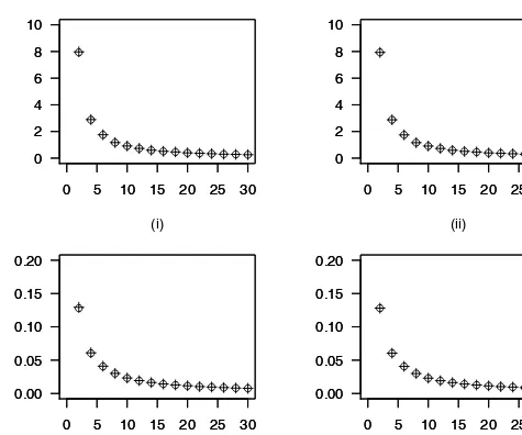
0 5 10 15 20 25 30 0 2 4 6 8 10 (i) 0 5 10 15 20 25 30 0 2 4 6 8 10 0 5 10 15 20 25 30 0 2 4 6 8 10 (ii) 0 5 10 15 20 25 30 0 2 4 6 8 10 0 5 10 15 20 25 30 0.00 0.05 0.10 0.15 0.20 (iii) 0 5 10 15 20 25 30 0.00 0.05 0.10 0.15 0.20 0 5 10 15 20 25 30 0.00 0.05 0.10 0.15 0.20 (iv) 0 5 10 15 20 25 30 0.00 0.05 0.10 0.15 0.20
Figure 2 – Monte Carlo variances of g x( )=x3+x2+ , ( ) , and x ( )s( 3 2 ; , , ) m
C x +x +x x a b , ( )+ , where a =1.5 and b =10, for random samples of size n =2,4,6, , 28,30… , from the folded nor-mal distribution; s =0.5 and m =4, in panel (i), s =2 and m =5, in panel (ii). Monte Carlo
vari-ances of 1 2 1 (x) ( 1) ( 1) g = x + − x + , ( ) , and ( ) 1 ms(( 2 1) ( 1 1); x, , ) C x + − x + a b , ( )+ , where a =1.5 and 10
b = , for random samples of size n =2,4,6, , 28,30… , from the bivariate folded normal distribu-tion; s =0.5 and m1=m2= , in panel (iii), 4 s =2 and m1=m2= , in panel (iv). 5
( ) 1 1 ms (( 2 1) ( 1 1); x, , ) ( 2 1) ( 1 1) C x + − x + a b = x + − x + 2 1 3 2 s ( 2 1) ( 1 1) m− − x − x + + + ' ' 1 2 { ( , )λ a b λ ( , )}a b ⋅ − ,
where 1/2s > − , and the quantity ' ' 1( , )a b 2( , )a b λ −λ is given by (7). We have ( ) 1 ( ) 1 ms (( 2 1) ( 1 1); x, , ) ms (( 2 1) ( 1 1); x, , ) C x + − x + a b =C x + − x + a b 3 2 2 ( s ) O m− − + , 1/2
s > − , as m → ∞ and 1 m → ∞ . The approximate Bernstein-type estimator 2
( ) 1
ms (( 2 1) ( 1 1); x, , )
( ) 1
ms (( 2 1) ( 1 1); x, , )
C x + − x + a b with the denominator of the function that was re-placed by its three-term Taylor expansion around x +2 1. See Wong (2001),
chap-ter 5, for further details about this procedure.
In Figure 2, we compare the Monte Carlo variances of 1
2 1
(x) ( 1) ( 1)
g = x + − x +
and ( ) 1
ms (( 2 1) ( 1 1); x, , )
C x + − x + a b , for s =0.5, 2, m =4,5, and the sample sizes 2,4,6, , 28,30
n = … . The Monte Carlo variances were based on 10000 inde-pendent replications from the folded normal distribution. The empirical results were equivalent.
7. CONCLUDING REMARKS
1). The quantity ' ' 1( , )a b 2( , )a b
λ −λ , given by (7), is crucial for the numerical performance of the univariate Bernstein-type approximations ( )s ( ; , , )
m
C g x a b , de-fined as (8), where s > −1/2, and x D∈ ⊆R1, and for the numerical
perform-ance of the multivariate Bernstein-type approximations ( )
ms ( ; x, , )
C g a b , defined as (9), where s > −1/ 2, and x D∈ ⊆Rq. The function ' '
1( , )a b 2( , )a b
λ −λ , given by
(7), does not admit a minimizer, for a >0 and b >0. See Chong and Żak (1996), chapter 6. Space curves ( ( ), ( ), )a t b t t , where t E∈ , and E⊆R1, can be easily
drawn in order to determine specific degrees of approximation. See Montiel and Ros (2005), chapter 1. The degrees (10) and (11) of approximation of the Bern-stein-type approximations C( )ms ( ; , , )g x a b and Cm( )s ( ; x, , )g a b , given by (8) and (9),
respectively, where s > −1/2, x D∈ ⊆R1, and x D∈ ⊆Rq, can be better than the degrees of approximation of the Bernstein-type approximations, that are pro-posed in Pallini (2005), for values of a and b such that λ1'( , )a b −λ2'( , ) 1/4a b < .
2). More efficient results for the Bernstein-type approximations C( )ms ( ; , , )g x a b and Cm( )s ( ; x, , )g a b , defined as (8) and (9), respectively, where s > −1/2,
1
x D∈ ⊆R , and x D∈ ⊆Rq, can be obtained by over-skewing the beta p.d.f. ( , )beta a b , and the moments '
1( , )a b
λ and '
2( , )a b
λ of the beta-binomial p.d.f., given by (4) and (5). We can over-skew the beta p.d.f. beta a b( , ), by an ad-ditional parameter τ , with values τ> , by determining the beta p.d.f. 0
( , )
beta a bτ . The beta p.d.f. beta a b( , )τ is negatively skewed, for τ <b a−1 ,
and is positively skewed, for τ>b a−1 . From the definition (7) of
' '
1( , )a b 2( , )a b
λ −λ , under the condition a2τ+aτ+b2τ−b2 2τ ≤a2+ , it is seen a
that ' ' ' '
1( , )a b 2( , )a b 1( , )a b 2( , )a b
3). Rosenberg (1967) studies an application of the multivariate Bernstein poly-nomial B gm( ; x), given by (2), to the Monte Carlo evaluation of an integral. The same application can be organized for the multivariate Bernstein-type approximation in Pallini (2005) and for the multivariate Bernstein-type ap- proximation ( ) ms ( ; x, , ) C g a b , given by (9), where s > −1/2, m ( , ,1 )T q m m = … , and
x D∈ ⊆Rq. Most importantly, straightforward versions of the Bernstein-type
approximations ( )s ( ; , , ) m
C g x a b and ( )
ms ( ; x, , )
C g a b , given by (8) and (9), respec-tively, where s > −1/2, x D∈ , x D∈ , are both multivariate approximations for functions and approximate multivariate integrals of functions. Focussing on
( )
ms ( ; x, , )
C g a b , given by (9), where s > −1/2, x D∈ , let us suppose that we are interested in the evaluation of an integral
Dg(x)dx
∫
, where D⊆Rq. Inparticu-lar, we can start from an approximate integration rule of the form
( ) ( ) ms ( ms ; x, , )
C h a b , where s > −1/2, hm( )s :[0,1]q× →D R1, and apply a procedure
for a more efficient integration rule. See Wong (2001), and Hanselman and Little-field (2005), chapter 24.
4). In the Bernstein-type approximations Cm( )s ( ; , , )g x a b and Cm( )s ( ; x, , )g a b ,
given by (8) and (9), respectively, where s > −1/2, x D∈ and x D∈ , the lin- ear kernels m−s(m k t−1 − + , the linear kernels ) x m−s(m v x−1 − )+ and x
1
( )
s
i i i i i
m− m v− −x + can be substituted by nonlinear kernels, where x 0,1, ,
k= … m, 0,1, ,ki = … mi, 1, ,i= … , and x Dq ∈ , x ( , ,= x1 …xq)T∈D,
re-spectively.
5). The Bernstein-type approximation ( )
ms ( ; x, , )
C g a b , given by (9), where 1/2
s > − , and x D∈ ⊆Rq, can be generalized by using a different
approxima-tion coefficient for each component. That is, we can use s ( , , )= s1… sq T in the
Bernstein-type approximation (s)
m( ; x, , )
C g a b , where x D∈ ⊆Rq. Another
gener-alization of the Bernstein-type approximation ( )
ms ( ; x, , )
C g a b , given by (9), where x D∈ ⊆Rq, can be based on
q
different beta-binomial p.d.f.’s, ( ; , )m i i
p k a b , that can be defined from (3), for every i= … . 1, ,q
6). Following DeVore and Lorentz (1993), chapter 1, it can be shown that the Bernstein-type approximation ( )s ( ; , , )
m
C g x a b , given by (8), is an integral operator with uniform convergence, as m → ∞ . If we suppose that ( ) 0g x ≠ ,
for every x D∈ , then we obtain ( ) 1
0 ( ; , , ) ( , ) ( ) s m m C g x a b =
∫
h t x g t dt , where 1 1 1 1 1 0 ( , ) { ( )} { ( , )} m ( s( ) ) a k (1 )b m k m k h t x = g x − B a b −∑
= g m− m k t− − +x t + − −t + − − is thekernel of this integral operator, s > −1/2, [0,1]t ∈ , and x D∈ . The definition of
( )s ( ; , , ) m
C g x a b by ( , )h t x , [0,1]m t ∈ , is equivalent to the problem of approximat-ing { ( )}g x 2 with ( )s ( ; , , )
m
C g x a b , where x D∈ . Similar results can be obtained for the multivariate Bernstein-type approximation ( )
ms ( ; x, , )
C g a b , given by (9), as i
m → ∞ , i= … . 1, ,q
7). Variants of the Bernstein polynomials that are discussed and studied in DeVore and Lorentz (1993), chapter 10, can also be regarded as extensions to the use of the binomial p.d.f. in Bernstein-like approximations. We recall that the most special cases of the beta p.d.f. are the arcsine distribution, the power distri-bution and the unform distridistri-bution. See Balakrishnan and Nevzorov (2003), chapter 16. Extensions to the beta-binomial p.d.f. p k a b , given by (3), where m( ; , )
0,1, ,
k= … m, are discussed and studied in Wilcox (1981). 8. APPENDIX
8.1. Basic properties of the Bernstein-type approximations (8) and (9) The Bernstein-type approximations ( )s ( ; , , )
m
C g x a b and (s)
m( ; x, , )
C g a b , given by (8) and (9), respectively, where s > −1/2, x D∈ and x D∈ , respectively, are lin-ear positive operators. Let γ1 and γ2 be finite constants. Let g , g , and 1 g be 2
functions, ( )g x , g x , and 1( ) g x , x D2( ) ∈ . We have
( ) ( ) 1 2 1 2 ( ; , , ) ( ; , , ) s s m m C γ +γ g x a b = +γ γ C g x a b ( ) ( ) ( ) 1 2 1 2 ( ; , , ) ( ; , , ) ( ; , , ) s s s m m m C g +g x a b =C g x a b +C g x a b ,
where s > −1/2, x D∈ . If g x1( )≤ g x2( ), for all x D∈ , we have
( ) ( ) 1 2 ( ; , , ) ( ; , , ) s s m m C g x a b ≤C g x a b ,
x D∈ . Multivariate versions of these properties hold for C(s)m( ; x, , )g a b , given by
(9), where s > −1/2, x D∈ .
8.2. Uniform convergence of the Bernstein-type approximations (8) and (9)
The uniform norm g of the function ( )g x , where x D∈ , is defined as max ( )
x D
g g x
∈
= . The Bernstein-type approximation ( )s ( ; , , ) m
C g x a b , where
x D∈ , is given by (8). We want to show that, given a constant ε> , there exists 0 a positive integer m , such that 0
0 ( )s ( ; , , ) ( ) m C g x a b −g x < , (18) ε for every x D∈ . For every x D∈ , ( )s (1; , , ) 1 m
C x a b = , where s > −1/ 2. We define the func- tions µ1( )x = and x µ2( )x =x2. We have Cm( )s ( ( ); , , )µ1 x x a b = , and x
( ) 2 1 ' ' 2
2 1 2
( ( ); , , ) { ( , ) ( , )}
s s
m
C µ x x a b =m− − λ a b −λ a b +x , where s > −1/2, and the
quantity ' '
1( , )a b 2( , )a b
λ −λ is given by (7).
Suppose that g =M. We take x0∈ . We have D
0
2M g x( ) g x( ) 2M
− ≤ − ≤ , (19)
where x x D0, ∈ . The function g is continuous; given ε1> , there exists a con-0
stant 0δ > , such that
1 g x( 0) g x( ) 1
ε ε
− < − < , (20)
for x0−x < , and δ x x D0, ∈ . From (19) and (20), it follows that
1 2M g x( 0) g x( ) 1 2M ε ε − − ≤ − ≤ + , and then 2 2 2 2 1 2M (x0 x) g x( 0) g x( ) 1 2M (x0 x) ε δ− ε δ− − − − ≤ − ≤ + − , (21)
for x x D0, ∈ . In fact, if |x0− < , (20) implies (21), x| δ x x D0, ∈ . If 0 |x − ≥ , then x| δ 2 2 0 (x x) 1 δ− − ≥ and (19) implies (21), 0, x x D∈ . Following Appendix 8.1, (21) becomes 2 ( ) 2 ( ) 1 2M Cms ( (x0 x) ; , , )x a b Cms ( ; , , )g x a b g x( ) ε δ− − − − ≤ − 2 ( ) 2 1 2M Cms ((x0 x) ; , , )x a b ε δ− ≤ + − , (22)
for x x D0, ∈ . We observe that (x0−x)2=x02−2x x x0 + 2, x x D0, ∈ . It
fol-lows that ( ) 2 2 1 ' ' 0 1 2 (( ) ; , , ) { ( , ) ( , )} s s m C x −x x a b =m− − λ a b −λ a b , (23)
for x D∈ , where the quantity ' ' 1( , )a b 2( , )a b λ −λ is given by (7). We have ( ) 2 2 1 0 (( ) ; , , ) ( ) s s m C x −x x a b =O m− − , as m → ∞ , x D∈ . Finally, we have ( ) 2 2 1 ' ' 1 1 2 ( ; , , ) ( ) 2 { ( , ) ( , )} s s m C g x a b −g x ≤ +ε Mδ− m− − λ a b −λ a b ,
x D∈ , where the quantity λ1'( , )a b −λ2'( , )a b is given by (7). Setting ε1=ε/2, for
any m0 >[4Mδ ε−2 −1{ ( , )λ1' a b −λ2'( , )}]a b 1/( 2 1)s+ , where s > −1/2, and the
quan-tity λ1'( , )a b −λ2'( , )a b is given by (7), the uniform convergence (18) is proved.
The condition s > −1/ 2 is required for the uniform convergence. The conver-gence C( )ms ( ; , , )g x a b → g x( ), for s > −1/ 2, is uniform, at any point of continuity
x D∈ , as m → ∞ , in the sense that the upper bound (23) for the uniform norm does not depend on x , x D∈ .
The multivariate Bernstein-type approximation Cm( )s ( ; x, , )g a b , where
1/2
s > − , and x D∈ , is given by (9). We observe that q is fixed and does not depend on m . Considering the uniform norm g of the function (x)g , x D∈ , defined as
x D
max (x)
g g
∈
= , we want to show that, given a constant ε> , there 0 exist positive integers m0 =(m01, ,… m0q)T, such that
0 ( )
ms ( ; x, , ) (x)
C g a b −g < , (24) ε
for every x D∈ .
For every x D∈ , C( )ms (1; x, , ) 1a b = , where s > −1/2. We define 1
1 (x) q i i x µ = =
∑
and 2 2 1 (x) q i i x µ = =∑
. We have ( ) m 1 1 ( (x); x, , ) q s i i C µ a b x = =∑
, and ( ) 2 1 ' ' 2 m 2 1 2 1 1 ( (x); x, , ) { ( , ) ( , )} q q s s i i i i C µ a b m− + λ a b λ a b x = = ⎛ ⎞ =⎜ ⎟ − + ⎝∑
⎠∑
, where s > −1/ 2, and the quantity ' ' 1( , )a b 2( , )a b λ −λ is given by (7).Suppose that g =M. We take x0=(x01, ,… x0q)T, where x0∈ . We ob-D
serve that 2 2 2 0 0 0 1 (|x x|) ( 2 ) q i i i i i x x x x =
− =
∑
+ − , x ,x D0 ∈ . The uniformconver-gence (24) follows from ( ) 2 2 1
m 0 1 ((|x x|) ; x, , ) ( ) q s s i i C a b O m− − = − =
∑
, as m → ∞ , for i 1/2s > − , where i= … , 1, ,q x ,x D0 ∈ . Under the condition s > −1/2, the
con-vergence ( )
ms (g;x, , ) (x)
C a b →g is uniform at any point of continuity x D∈ , as
i
m → ∞ , where i = … . 1, ,q
8.3. Degrees of approximation (10) and (11)
equal to 1 0
x x
δ− − , where
0,
x x D∈ . We recall the definition of the modulus of continuity ( )ω δ , where δ > . We have 0
0 0
( ) ( ) ( ){1 ( , ; )}
g x −g x ≤ω δ +ξ x x δ , (25)
0,
x x D∈ .
The Bernstein-type approximation ( )s ( ; , , )
m
C g x a b is given by (8), where 1/2
s > − , and x D∈ . Then, we have that
( )s ( ; , , ) ( ) m C g x a b −g x 1 1 1 1 1 0 0 { ( , )} m ( s( ) ) ( ) a k (1 )b m k k m B a b g m m v t x g x t t dt k − − − + − + − − = ⎛ ⎞ ≤ − + − ⎜ ⎟ − ⎝ ⎠
∑
∫
1 1 1 1 0 0 0 ( ){ ( , )} m{1 ( , ; )} a k (1 )b m k k m B a b x x t t dt k ω δ − ξ δ + − + − − = ⎛ ⎞ ≤ + ⎜ ⎟ − ⎝ ⎠∑
∫
1 1 1 1 1 1 0 0 ( ){ ( , )} m{1 s( ) } a k (1 )b m k k m B a b m m k t t t dt k ω δ − δ− − − + − + − − = ⎛ ⎞ ≤ + − ⎜ ⎟ − ⎝ ⎠∑
∫
1 1 1 2 2 2 2 1 0 0 ( ){ ( , )} m{1 s ( ) } a k (1 )b m k k m B a b m k mt t t dt k ω δ − δ− − − + − + − − = ⎛ ⎞ ≤ + − ⎜ ⎟ − ⎝ ⎠∑
∫
, x D∈ . It follows that ( ) 2 2 1 ' ' 1 2 ( ; , , ) ( ) ( )[1 { ( , ) ( , )}] s s m C g x a b −g x ≤ω δ +δ− m− − λ a b −λ a b ,x D∈ . Setting δ =m−1/2, we finally have the degree of approximation (10).
For every δ > , we denote by 0 ξ(x ,x; )0 δ the maximum integer less than or
equal to 1 0 x x δ− − , where 1/2 2 1 1 0 0 1 x x q ( i i) i x x δ− δ− = ⎛ ⎞ − = ⎜ − ⎟ ⎝
∑
⎠ , and x , x D0 ∈ . We have g(x )0 −g(x) ≤ω( ){1δ +ξ(x ,x; )}0 δ , where ( )ω δ is the modulus ofcontinuity, 0δ > , and x , x D0 ∈ .
The multivariate Bernstein-type approximation ( )
ms ( ; x, , )
C g a b is given by (9), where s > −1/2, and x D∈ . We have
( ) 2 2 1 ' ' m 1 2 1 ( ; x, , ) (x) ( ) 1 q { ( , ) ( , )} s s i i C g a b g ω δ δ− m− − λ a b λ a b = ⎡ ⎤ − ≤ ⎢ + − ⎥ ⎣
∑
⎦,x D∈ . Setting δ =m−1/2, where 1 q i i m m =
=
∑
, we finally have the degree of ap-proximation (11).8.4. Orders of error in probability (14) and (15)
The Bernstein-type approximation ( )s ( ; , , )
m
C g x a b is given by (12), where 1/2
s > − . Let g x′( ) ( )= dx −1dg x( ) and g x''( ) ( )= dx −2 2d g x( ) be the first two derivatives of the function ( )g x , where x D∈ . We recall that the quantity
' '
1( , )a b 2( , )a b
λ −λ is given by (7). By Taylor expanding the function
1
( s( ) )
g m− m k t− − +x around µ, for every k=0,1, ,… m, we have
( )s ( ; , , ) ( ) m C g x a b = g µ '( )( ) g µ x µ + − 2 1 ' ' 2 1 2 1 [ ''( ) { ( , ) ( , )} ''( )( ) ] 2 s g µ m− − λ a b λ a b g µ x µ + − + − + 1/2 2 1 ( ) ( ) ( s ) p g µ O n− O m− − = + + ,
where s > −1/ 2, as m → ∞ , and n → ∞ . Order ( 2 1s ) ( 1/2) p
O m− − +O n− of error in probability in (14), as m → ∞ , and n → ∞ , is thus proved.
The Bernstein-type approximation Cm( )s ( ; x, , )g a b is given by (13), where
1/ 2
s > − . By Taylor expanding the function
1 1 1 1 1 1 1 ( ) ( ) s s q q q q q m m k t x g m m k t x − − − − ⎛ − + ⎞ ⎜ ⎟ ⎜ ⎟ ⎜ ⎟ ⎜ − + ⎟ ⎝ ⎠ around ( , ,1 )T q
µ= µ … µ , for every ki = …1, ,mi, i= … , we can prove the 1, ,q
order 2 1 1/2 1 ( ) ( ) q s i p i O m− − O n− = +
∑
of error in probability in (15), s > −1/2, as i m → ∞ , where i = … , and n → ∞ . 1, ,q8.5. Asymptotic normality (16) and (17)
Following (14), we have that 1/2{ ( )s ( ; , , ) ( )} m
n C g x a b −g µ , where s > −1/2, is asymptotically equivalent to n1/2{ ( )g x −g( )}µ , as m → ∞ and n → ∞ . An
ap-plication of the Central Limit Theorem then shows the asymptotic normality in (16), as m → ∞ , and n → ∞ .
Following (15), we have n1/2{Cm( )s ( ; x, , )g a b −g( )}µ , where s > −1/2, 1
m ( , ,= m … mq)T, is asymptotically equivalent to n1/2{ ( x)g −g( )}µ , as m → ∞ , i
where 1, ,i= … , and n → ∞ . An application of the Central Limit Theorem then q shows the asymptotic normality in (17), as m → ∞ , where i i= … , and 1, ,q
n → ∞ .
Dipartimento di Statistica e Matematica ANDREAPALLINI
Applicata all’Economia Università di Pisa
REFERENCES
N. BALAKRISHNAN, V.B. NEVZOROV (2003), A primer on statistical distributions, Wiley and Sons,
New York.
O.E. BARNDORFF-NIELSEN, D.R. COX (1989), Asymptotic techniques for use in Statistics, Chapman &
Hall, London.
R.A. BECKER, J.M. CHAMBERS, A.R. WILKS (1988), The new S Language, Wadsworth and Brooks/
Cole, Pacific Grove, California.
E.W. CHENEY (1982), Introduction to approximation theory, 2nd Edition, AMS Chelsea
Publish-ing, American Mathematical Society, Providence, Rhode Island.
E.K.P. CHONG, S.H. ŻAK (1996), An introduction to optimization, Wiley and Sons, New York. P.J. DAVIS (1963), Interpolation and approximation, Blaisdell Publishing Company, Waltham,
Massachusetts.
R.A. DEVORE, G.G. LORENTZ (1993), Constructive approximation, Grundlehren der
mathema-tischen Wissenschaften 303, Springer-Verlag, Berlin.
W. FELLER (1968), An introduction to probability theory and its applications, Volume I, 3rd
Edi-tion, Wiley and Sons, New York.
W. FELLER (1971), An introduction to probability theory and its applications, Volume II, 2nd
Edi-tion, Wiley and Sons, New York.
P. HALL (1992), The bootstrap and edgeworth expansion, Springer-Verlag, New York.
D. HANSELMAN, B. LITTLEFIELD (2005), Mastering MATLAB®7, Pearson Prentice Hall, Upper
Saddle River, New Jersey.
N.L. JOHNSON, A.W. KEMP, S. KOTZ (2005), Univariate discrete distributions, 3rd Edition, Wiley and
Sons, New York.
N.L. JOHNSON, S. KOTZ, S. BALAKRISHNAN (1997), Discrete multivariate distributions, Wiley and
Sons, New York.
P.P. KOROVKIN (1960), Linear operators and approximation theory, Hindustan Publishing
Corpo-ration, Delhi.
S. MONTIEL, A. ROS (2005), Curves and surfaces, AMS Graduate Studies in Mathematics 69,
American Mathematical Society, Real Sociedad Mathemàtica Española, Providence, Rhode Island.
F.W.J. OLVER (1997), Asymptotics and special functions, A. K. Peters, Natick, Massachusetts. A. PALLINI (2005), Bernstein-type approximation of smooth functions, “Statistica”, 65, 169-191. G.M. PHILLIPS (2003), Interpolation and approximation by polynomials, Springer-Verlag, New
York.
R.J. RIVLIN (1981), An introduction to the approximation of functions, Reprint of the 1969 Edition,
Dover Publications, Mineola, New York.
L. ROSENBERG (1967), Bernstein polynomials and Monte Carlo integration, “SIAM Journal of
Nu-merical Analysis”, 4, 566-574.
P.K. SEN, J.M. SINGER (1993), Large Sample Methods in Statistics: An introduction with applications,
Chapman & Hall, New York.
R.R. WILCOX (1981), A review of the Beta-Binomial model and its extensions, “Journal of
Educa-tional Statistics”, 6, 3-32.
R. WONG (2001), Asymptotic approximations of integrals, Reprint of the 1989 Edition, SIAM
Classics in Applied Mathematics 34, Society for Industrial and Applied Mathematics, Philadelphia.
SUMMARY
Bernstein-type approximation using the beta-binomial distribution
The Bernstein-type approximation using the beta-binomial distribution is proposed and studied. Both univariate and multivariate Bernstein-type approximations are studied. The uniform convergence and the degree of approximation are studied. The Bernstein-type estimators of smooth functions of population means are also proposed and studied.

![[Recensione a] Rosanna Scatamacchia. Azioni e azionisti. Il lungo Ottocento della Banca d'Italia, Roma-Bari, Laterza, 2008](data:image/gif;base64,R0lGODlhAQABAIAAAP///wAAACH5BAEAAAAALAAAAAABAAEAAAICRAEAOw==)