An Analysis of Eye Scanpath Entropy in a Progressively Forming Virtual Environment

London WC1E 6BT, UK Mel Slater*

Department of Computer Science University College London London WC1E 6BT, UK and

ICREA—University of Barcelona EVENT Lab, Facultat de Psicologia, Campus de Mundet Edifici Teatre, Passeig de la Vall d’Hebron 171, 08035 Barcelona, Spain

Presence, Vol. 18, No. 3, June 2009, 185–199 ©2009 by the Massachusetts Institute of Technology

Forming Virtual Environment

Abstract

A sign of presence in virtual environments is that people respond to situations and events as if they were real, where response may be considered at many different levels, ranging from unconscious physiological responses through to overt behavior, emotions, and thoughts. In this paper we consider two responses that gave differ-ent indications of the onset of presence in a gradually forming environmdiffer-ent. Two aspects of the response of people to an immersive virtual environment were re-corded: their eye scanpath, and their skin conductance response (SCR). The sce-nario was formed over a period of 2 min, by introducing an increasing number of its polygons in random order in a head-tracked head-mounted display. For one group of experimental participants (n⫽ 8) the environment formed into one in which they found themselves standing on top of a 3 m high column. For a second group of participants (n⫽ 6) the environment was otherwise the same except that the column was only 1 cm high, so that they would be standing at normal ground level. For a third group of participants (n⫽ 14) the polygons never formed into a meaningful environment. The participants who stood on top of the tall column ex-hibited a significant decrease in entropy of the eye scanpath and an increase in the number of SCR by 99 s into the scenario, at a time when only 65% of the poly-gons had been displayed. The ground level participants exhibited a similar decrease in scanpath entropy, but not the increase in SCR. The random scenario grouping did not exhibit this decrease in eye scanpath entropy. A drop in scanpath entropy indicates that the environment had cohered into a meaningful perception. An in-crease in the rate of SCR indicates the perception of an aversive stimulus. These results suggest that on these two dimensions (scanpath entropy and rate of SCR) participants were responding realistically to the scenario shown in the virtual envi-ronment. In addition, the response occurred well before the entire scenario had been displayed, suggesting that once a set of minimal cues exists within a scenario, it is enough to form a meaningful perception. Moreover, at the level of the sympa-thetic nervous system, the participants who were standing on top of the column exhibited arousal as if their experience might be real. This is an important practical aspect of the concept of presence.

*Correspondence to m.slater@cs.ucl.ac.uk.

1 Introduction

The success of many applications of immersive virtual environments (IVEs) depends on the extent to which participants respond to situations and events in the VE similarly to how they would respond in a corre-sponding physical environment. Obvious applications are training for real-world tasks (Brooks, 1999), and also various forms of therapy and rehabilitation (Rizzo & Kim, 2005). The concept of presence has usually been used to describe the feeling of being there that people report after experiences within IVEs (Sheridan, 1992); but rather than only being considered as a purely subjective phenomenon, this term has been extended to include this notion of response as-if-real (Sanchez-Vives & Slater, 2005). Therefore, a valid research task is to understand the conditions under which people will tend to respond as-if-real (RAIR), irrespective of their subjec-tive reporting about their state of being there. Such RAIR is applicable with respect to many dimensions, ranging from unconscious physiological responses through to observable behavioral responses, emotions, and thoughts, and of course, participants in an IVE may exhibit RAIR on some dimensions but not others. Of particular interest are those responses that are objec-tively measurable. In this paper we examine two directly measurable aspects of RAIR, eye scanpath entropy and skin conductance changes in response to a stressful situ-ation, where the eye scanpath refers to the fixations of the eye and the transitions between them and the result-ing path over some stimulus.

An additional goal of the research was to investigate whether a person’s eye scanpath changes at the moment that the virtually generated visual sense data forms into a meaningful perception. In order to know when this perception is formed, the scenario that the participant eventually could perceive is one that in physical reality would represent danger. Changes in physiological re-sponses that would indicate a sudden recognition of danger therefore served as a marker of environment per-ception. It also served as a marker for RAIR, since the change in sympathetic nervous system response indi-cates that the danger was perceived. This change in

re-sponse only makes sense if participants were at this basic level responding to the environment as if it were real.

This research is part of a wider attempt to understand how people respond to situations and events within IVEs. We are particularly interested in the circumstances under which people respond as if what they were per-ceiving were real, even though they are fully aware that it is only in an IVE. The literature provides many exam-ples of people responding realistically to virtual situa-tions and events. In particular, it has been demonstrated that people respond with anxiety to virtual stressful situ-ations. For example, a visual cliff type of environment has been used where participants were confronted with a VE that depicts a precipice, and their heart rate in-creased significantly (Meehan, Insko, Whitton, & Brooks, 2002; Meehan, Razzaque, Whitton, & Brooks, 2003). Skin conductance, heart rate, and heart rate vari-ability have been shown to respond significantly in the context of general social situations (Slater, Guger, et al., 2006), and social situations that are highly stressful (Slater, Antley, et al., 2006). It has also been found that there are similarities in behavior when participants play handball in virtual reality compared to physical reality (Bideau et al., 2003). In these examples, anxiety, as measured through physiological responses, is one sign that people are responding to the virtual events as if they were really happening. Using changes in eye scan-paths in conjunction with changes in physiological mea-sures provides an additional way to explore how people respond.

Here we describe an experiment in which participants are placed into a VE that develops, by polygons being randomly added over time, until it becomes a well-formed recognizable scenario in which participants eventually realize that they are standing on top of a col-umn. There were three conditions: In the experimental condition the column is very high, so that an anxiety response would be expected once the participants per-ceived their location. In the control condition the col-umn height is at ground level. We recorded electroder-mal activity (EDA) and the eye scanpaths of the participants. From the EDA, we compute the number of skin conductance responses (SCRs; Dawson, Schell, & Filion, 2000). We find that at the time that

partici-pants in the experimental condition must have recog-nized that they are standing on a high column, the SCR rate increases significantly, and the entropy of the eye scanpath decreases significantly. For those in the control condition, the SCR rate does not change, but the eye scanpath entropy also decreases significantly. Finally, for a third random condition where the environment re-mains random throughout, the eye scanpath entropy does not decrease. These results taken together suggest that eye scanpath entropy may be used to indicate the moment at which a virtual scenario becomes perceptu-ally stable, in the sense that an observer has started to employ gaze direction sensorimotor contingencies cor-responding to those that would be used for visual per-ception of a real place.

In the next section we discuss the relevant eye scan-path perception literature. In Section 3 we describe the experiment in detail, and in Section 4 the results. We discuss the results as they relate to the research objectives and context in Section 5, with conclusions in Section 6.

2 The Eye Scanpath and Perceptual Selection

The visual perception literature is concerned with both bottom-up and top-down modeling of the percep-tual process (Goldstein, 2002; Henderson, 2007). Top-down processing describes a perceptual system that is driven by high-level cognition relying upon a person’s prior experience (Gregory, 1998; Rao, Zelinsky, Hay-hoe, & Ballard, 2002). Conversely, bottom-up process-ing is used to describe the perceptual system as moti-vated by the sensory stimuli arriving at receptors (Itti & Koch, 2000). It is commonly thought that such systems cooperate to achieve perception (Goldstein, 2002; Tor-ralba, Oliva, Castelhano, & Henderson, 2006; Ware, 2008). However, here we concentrate primarily on top-down processes.

Our approach follows the idea of selection between alternative perceptual hypotheses (real world, virtual world). The concept of perceptual hypothesis selection is based on the work of Gregory (1998), which asserts that (visual) perception works through an ongoing

se-lection between competing top-down hypotheses insti-gated by some visual stimulus. These hypotheses are said to arise from high-level conceptual models rather than from low-level stimuli directly— hence the term top-down. An explicit example of the competition of top-down hypotheses would be in viewing ambiguous images such as the Necker cube, when the ambiguous stimuli leads to an instability of perception, and the per-ception switches between alternative percepts. But it should be noted that earlier, Gregory also stated (1977) that a total lack of a superior hypothesis leads to a lack of perception.

This model of competing top-down hypotheses pro-vides one explanation as to why people tend to respond realistically within IVEs in spite of the fact that they are usually poor representations of reality. This is because the perception of the virtual environment provides the best hypothesis for interpreting the stimuli, and so even low fidelity virtual environments may contain sufficient cues to trigger the desired perceptual hypothesis. Top-down perceptual selection was implied when a link be-tween ambiguous stimuli and virtual reality was first proposed by Stark (1995), to explain “How Virtual Re-ality Works!” Stark had previously investigated eye movements when viewing illusory ambiguous figures, including the Necker cube, and found that a person’s eye movements were related to what was being per-ceived rather than simply the objective content of the visual stimuli (Stark & Ellis, 1981). An application of these ideas to presence was discussed by Slater (2002).

The idea of “sufficient cues” begs the question as to whether there exists a set of minimal cues. It has been suggested that there might be a threshold level of fidel-ity beyond which people would experience presence. This was referred to as the minimal set of cues (minimal cues; Slater, 2002; Sanchez-Vives & Slater, 2005). If they exist, minimal cues would play an important role in understanding people’s responses in virtual environ-ments, because the threshold for RAIR could then be systematically investigated through controlled experi-ments. Apart from these two texts, minimal cues have not been specifically discussed and are only mentioned fleetingly in presence research. There is, however, indi-rect evidence for the idea. For example, Zimmons and

Panter (2003) found that increasing rendering quality did not appear to increase responses to an anxiety pro-voking environment. It has also been found (Mania & Robinson, 2004) that reported presence was not signifi-cantly different between three conditions rendered at varying levels of quality. These results could imply that the threshold had already been reached, and thus no longer increased presence responses.

Buswell (1935) demonstrated that when observing a complex visual stimulus, eye movements are dependent upon the stimulus itself. He showed this by systemati-cally recording the eye movements of experimental par-ticipants while they viewed more than 50 pictures, which led to the finding that fixations were grouped around salient features in the pictures. In the later work of Yarbus (1967) it was discovered that saccades (transi-tions between fixa(transi-tions) were also dependent upon the visual stimulus, and were highly repetitive.

However, although it had long been known that eye movements were dependent on the stimulus, Stark and Ellis (1981) found that a particular perception was char-acterized by idiosyncratic and repeated fixations and saccades among the salient features of the visual stimu-lus. This path over the visual stimulus was termed a scanpath in the related earlier work of Noton and Stark (1971). It is possible that if minimal cues exist, they would be related to these salient features and repeated saccades of the scanpath.

3 Experimental Design

3.1 Scenario and Hypotheses An environment was designed representing a room in which there was a column. The environment consisted of 3500 polygons, but in our experiment, rather than the whole scenario being displayed immedi-ately, the polygons entered at random over time until the scenario was fully formed. We wished to investigate whether there would be a moment at which the ob-server suddenly perceived the meaning of the scenario, when it transformed from being a random set of poly-gons distributed in 3D space, to being perceived as a place. If the scenario was perceived as a place at some

time before it was fully formed, this would provide evi-dence in favor of minimal cues (through RAIR). How would we know when the participant had perceived the environment? In one version of the scenario the partici-pant would be standing on a column, 3 m above ground level. At the moment that this was realized, we would expect a change in skin conductance, since this would be a surprising and arousing event. At the same moment we would expect that the scanpath would become stabi-lized and repetitive, indicated by a decrease in its en-tropy (the same fixation points and saccades revisited, rather than random visual exploration of the environ-ment). For a similar environment, but where the partici-pant would be at ground level, we would expect no change in skin conductance but nevertheless a change in scanpath entropy. Finally, for an environment that never formed into a meaningful one (randomly distributed poly-gons only), we would expect no decrease in entropy.

A single-factor between-groups experimental design was therefore used. There were three environments, the stress-inducing environment, the no-stress environment, and the random environment.

Each group experienced their respective scenario that developed over time, with an exposure time of 4 min. During the first 2 min the environment developed dy-namically from an empty (black) void to its complete state. The environment was then static, remaining in this final state for the last 2 min. The duration of the experiment is relatively long in comparison to studies found in the eye movement literature, since in order to characterize the eye movements at different times (as the experiment progressed) we required a large number of eye fixations and saccades.

All environments consisted of the same set of poly-gons. The development over time of each environment entailed the addition of polygons belonging to the final state (added in a random order, but the same order for all participants). Each new set of polygons was added after an interval of 4 s, the number of polygons being added increasing exponentially after each period, until all polygons were displayed.

3.1.1 Stress-Inducing Environment. The stress-inducing environment is a simple room

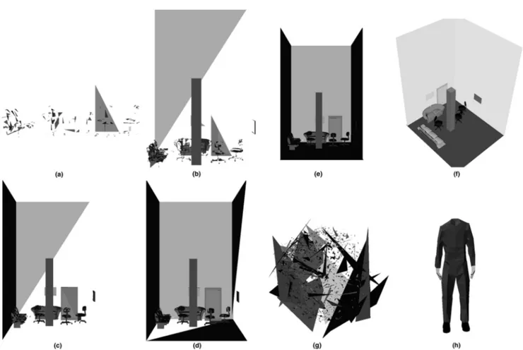
environ-ment containing everyday items of furniture, with the exception that it was designed specifically to induce ver-tigo by means of the inclusion of a tall column upon which the participant stands. Stages of the environ-ment’s development are shown in Figure 1(a– e), and the complete environment in Figure 1(f).

Specifically, the environment consists of a room mea-suring 3 m square and 6 m high. In the room are several items of furniture (three chairs and two sofas), a door, and two empty picture frames on the wall. Also, in the center of the room is a column of width and length of 40 cm, and a height of 3 m, upon which is stood the virtual body of the participant. The environment was presented such that participants would view it from a standing position on top of the column, that is, from the position of the eyes of their virtual body.

3.1.2 No-Stress Environment. The no-stress environment is a direct copy of the stress-inducing envi-ronment except that the column’s height was reduced to 1 cm (appearing as a simple square mat beneath the partici-pant’s feet) to provide a neutral (no vertigo) condition.

The virtual body and viewpoint were also displaced accordingly, so that the participant viewed the room from the top of the virtual body that thus was standing upon the floor of the room.

3.1.3 Random Environment. The random envi-ronment also contained the same polygons as the stress-inducing environment (and hence also the no-stress en-vironment), but they were rotated randomly about the center of the model to create a meaningless scene. The result is shown as Figure 1(g).

Figure 1. Stress-inducing environment at varying levels of detail (a) ... (b) ... (f). Random environment at highest level of detail (g). Participants’

In all three environments, the virtual body was sup-plied in the form of a headless avatar extending from the floor of the physical lab up to just below the center of projection (where their head would be). This is shown as Figure 1(h). Hence, when the participant looked down he or she would see a virtual trunk, legs, and feet, approximately registered where their real body would be.

3.2 Procedures

Subsequent to approval of our experiment by the UCL Ethics Committee, participants with good and uncorrected eyesight were recruited by advertisements placed around the University College London campus. Participants were asked to take part in a paid virtual real-ity study entitled “Investigating Environments,” lasting approximately 45 min in total. Twenty-eight (N⫽ 28) participants both qualified and completed the experi-ment satisfactorily, nSE⫽ 8 (stress-inducing

environ-ment), nNE⫽ 6 (no-stress environment), nRE⫽ 14

(random environment). Within each condition the number of male and female participants was equal.

Before each trial was carried out, the participant com-pleted a general demographic questionnaire and a simu-lator sickness questionnaire (SSQ; Kennedy, Lane, Ber-baum, & Lilienthal, 1993). They then put on the equipment. Next, the participant followed a standard (Applied Science Labs 501) procedure to calibrate the eye-tracking equipment. Once completed, they were directed to stand over a floor marker set at a place corre-sponding to that at which the virtual body stood. They were next shown a training environment that consisted of everyday items of furniture along with the virtual body. The training environment was used to test the equip-ment, allow the participants to get used to wearing it, and also to record baseline data for each type of mea-sure we used.

After viewing the training environment, it was ex-plained to the participant that their task would be to look for a small flower (although no flower was ever presented). This task was given to participants to en-courage them to visually explore the scene. The partici-pants were required to keep their feet planted in the same spot throughout the experiment, but were

other-wise allowed to move their body and limbs. The experi-ment was then started; and it lasted a total of 4 min.

After the trial, the eye tracker calibration was checked in case the eye tracker had slipped so as to render the data unusable. The participants were then able to remove the equipment, and were asked to complete a second simula-tor sickness questionnaire (Kennedy et al., 1993) and a presence questionnaire (Slater & Steed, 2000).

3.3 Materials

A 1.8 GHz PC drives the main application (graph-ics). The VE was displayed using a Virtual Research VR8 head mounted display (HMD), coupled to a Pol-hemus Fastrak head tracker. The HMD is used to dis-play color stereo images, having a refresh rate of 60 Hz, and a resolution of 640 by 400 pixels per screen. The viewing angle is 60° across the diagonal. The Polhemus Fastrak is a 6 DOF tracker used to track the head posi-tion and orientaposi-tion at a rate of 120 Hz.

Attached to the HMD is a single camera-based eye-tracker (ASL 501) for the left eye, that updates at a fre-quency of 50 Hz (constrained by the camera’s refresh rate).

A ProComp⫹ physiological instrument was used to measure skin conductance sampled at a rate of 32 Hz.

All data from the above devices were recorded, as well as the times of each event—an event being defined as the appearance of a set of polygons in the environment. A separate SGI O2 machine was used to record all data via VRPN software (Taylor et al., 2001).

3.4 Response Variables

The two main response variables of interest were derived from electrodermal activity (EDA) and compos-ite eye-head movements. In addition there were re-sponses to the presence questionnaire.

3.4.1 Electrodermal Activity. The EDA data was recorded as skin conductance (in␮Siemens) at a rate of 32 Hz. The measure used was the number of skin conductance responses (SCRs) computed as fol-lows: First the signal was smoothed, which was achieved

through the use of a wavelet decomposition function that effectively acts as a low-pass filter. Decomposition at six levels was performed, and then a reconstruction of the wavelet coefficients at the greatest level that pro-vides us with an error of less than 0.05␮Siemens is se-lected as the new series. The error in this case is defined as the maximum spot difference between the original data series and the reconstructed (smooth) series. The second order derivative of this smoothed series indicates the points in time at which the signal accelerates and decelerates (i.e., maximal turning points), these being identified as potential SCRs. An SCR was defined using this method as a local maximum that has an amplitude greater than 0.2␮Siemens occurring within a window of 5 s (Dawson et al., 2000).

Our first response variable S(t) is determined by com-puting the number of these SCRs that occur in the in-terval (t–30, t] for each t⫽ 30. . . 209. This may be described as a discrete 30-s sliding window with a reso-lution of 1 s.

3.4.2 Eye-Head Movements. The second re-sponse variable is designed to reflect the entropy of eye-head movements over a relatively short period of time. This is achieved through the analysis of the participant’s line-of-sight in 3-space, which is traced as it moves around the scene, and is calculated from the composite eye-tracking and head-tracking data.

The scene is segmented into 80 regions using a geo-desic grid (described below), and transitions of the line-of-sight between regions are recorded. A transition to a region is only assumed after the region has been fove-ated for a period longer than 267 ms (Buswell, 1935). Other temporal thresholds were also tried (Duchowski, 2003; Yarbus, 1967), but these made little difference, as there were only negligible changes in the resulting fove-ation sequences. A state-state transition frequency ma-trix is then constructed, from which the entropy rate may be computed, which is our response variable. This method is inspired by the work of Ellis and Stark (1986) which provides a method by which we may compute a statistical dependency metric. In this paper we are not attempting to reproduce their results, but we find in

their work a metric that characterizes a transition matrix in exactly the way we require. It should be noted that our study has quite different conditions, for instance, using head tracking our scene extends 360° around the subject, and thus we use larger regions that cover ele-ments of an environment. In contrast, Ellis and Stark’s paper utilized a spatially fixed image that subtends an acute solid angle.

Icosahedrons are a typical polyhedron used to create a geodesic grid. Although it only has 20 sides, it may be easily and regularly subdivided (increasing the number of faces by a factor of 4). For our purposes, there is a trade-off between too few faces (not enough detail cap-tured) and too many faces (leading to large transition matrices). We felt that subdividing it just once would provide the maximum number of faces (80) that we could sample for in the experiment.

The icosahedron faces are thus subdivided once into four equilateral triangles to generate the geodesic grid that has 80 regions. Each vertex of the subdivided icosa-hedron is the endpoint of a vector from the center of the structure, and we normalize each of these so that all vectors have a length of 1 m—to ensure each vertex is then a point on a sphere. This structure is then placed around the observer to segment the scene, with each triangle acting as an invisible window onto each region of the environment.

Each triangle is numbered, and so as the line-of-sight passes from one region (triangle) to another, the transi-tion is recorded in a transitransi-tion frequency matrix.

From the transition frequency matrix, a transition probability matrix can then be created. The conditional entropy (or just entropy, used interchangeably in this paper) of such a transition matrix may be computed as follows (Brillouin, 1962): H⫽

冘

冉

冘

冊

1. we define pijas the probability of transitioning

from region i to j. It may be considered as the number of i to j transitions divided by the total number of transitions.

2. pi3jis defined as the conditional probability of

transitioning from region i to j, given that the line-of-sight is currently intersecting region i:

pi3j⫽

pij

冘

3. piis the marginal probability of foveating region i.

It is estimated as:

pi⫽

冘

It should be noted that a transition matrix is pro-duced using a number of observed transitions over time, and as such, H is computed over a sliding 30-s window at 1-s intervals. Specifically, we compute H(t) over the transitions recorded in the interval (t – 30, t], where t⫽ 30 . . . 209, and this forms our second response variable.

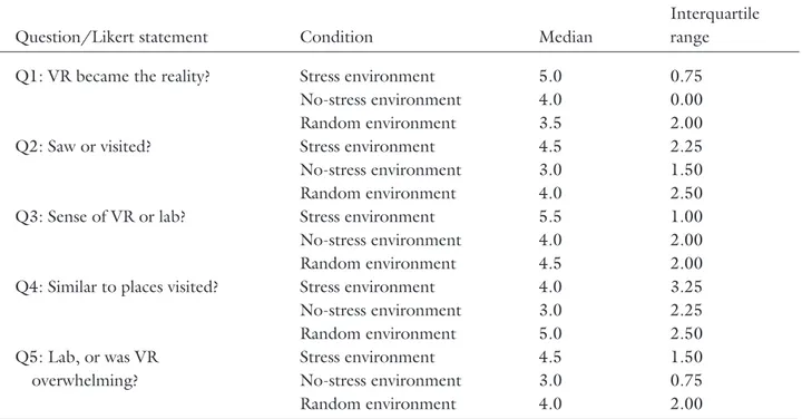
3.4.3 Questionnaire Response Variable. Apart from the response variables described above, a presence questionnaire was administered (Slater & Steed, 2000). This contains five presence related items, each measured on a 7-point Likert scale. The main focus of this study was the RAIR aspect of presence, and the subjective information was only recorded for completeness. The questions are shown in the Appendix.

4 Results

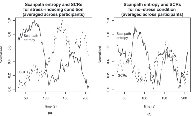
Figure 2 shows the number of SCRs and the scan-path entropy for each of the stress-inducing environ-ment and no-stress environenviron-ment conditions summed over all participants in the respective conditions. Each has been normalized so that they can be shown on the same graph. The graphs suggest that for the stress-Figure 2. Normalized scanpath entropy and SCR (averaged across all participants). (a) Stress-inducing environment; (b) no-stress environment.

inducing environment the number of SCRs rises at ap-proximately the same moment that the scanpath en-tropy starts to decline, indicating that at the time that the scene was perceptually formed, the participants ex-perienced the arousal invoked by the illusion of being on a column high above the ground. For the no-stress environment condition the scanpath entropy declines, but the graph does not suggest a similar corresponding increase in SCRs.

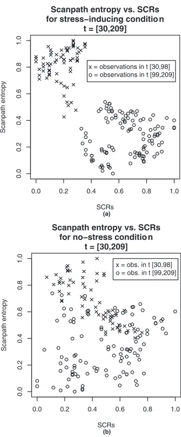
The most convincing result of the difference in the two conditions is provided in Figure 3, which shows a scatter plot of the normalized scanpath entropy against the SCRs. To form this figure, the scanpath entropy response variable Hk(t) is computed at each second (t⫽

30, . . ., 209), for each of the participants k⫽ 1, . . . , Ncondition(where Nconditionis the total number of

partic-ipants in some condition). These values are normalized (to be between 0 and 1) and then averaged across indi-viduals to produce the mean at each second:

Havg共t兲 ⫽

1

Ncondition

冘

In the same way we compute the number of SCRs, Sk(t), for each time t, and participant k; and then normalize

and average across participants to obtain Savg(t). Finally,

the values of Havg(t) and Savg(t) are plotted against each

other for each value of t to form the figures.

The stress-inducing condition (Figure 3a) shows the data as two distinct clusters; and by applying hierarchical clustering (with centroid linkage) we find that the upper left group (shown as crosses) contains observations over the interval [30, 98] exclusively, and the lower right group (shown as circles) observations over the interval [99, 209]. This indicates a discontinuity between 98 and 99 s, at which point the environment appeared as in Figure 4. Note that this is before the environment had been fully formed (at 120 s). There is no such clustering in the no-stress condition (Figure 3b).

4.1 Skin Conductance Response Results It is also important to show that the increase in SCRs and the decrease in scanpath entropy are both reflected by the individuals of the sample, and not only by their means.

0.0 0.2 0.4 0.6 0.8 1.0 0.0 0.2 0.4 0.6 0.8 1.0 SCRs Scanpath entropy Scanpath entropy vs. SCRs for stress−inducing conditio n

t = [30,209] x = observations in t [30,98] o = observations in t [99,209] (a) 0.0 0.2 0.4 0.6 0.8 1.0 0.0 0.2 0.4 0.6 0.8 1.0 SCRs Scanpath entropy Scanpath entropy vs. SCRs for no−stress conditio n

t = [30,209]

x = obs. in t [30,98] o = obs. in t [99,209]

(b)

Figure 3. Normalized scanpath entropy versus normalized SCRs—

each point being the result of averaging values across participants. (a) stress-inducing environment; (b) no-stress environment.

Table 1 shows the number of SCRs for each partici-pant, within a period of 90 s before and then after the discontinuity between clusters, between t⫽ [98, 99]. Our null hypothesis is that the median number of SCRs should be the same before and after. It can be seen that in the stress-inducing environment, the number of SCRs before the discontinuity is consistently less than the number afterward. Using the nonparametric sign test (one-sided), the null hypothesis is rejected (p⬍ .004). In the non-stress condition we cannot reject the null hypothesis (p⬍ .656).

4.2 Scanpath Entropy Results

Table 2 shows the scanpath entropy over the 90-s period before and then after the cluster-determined dis-continuity. To obtain these values for each participant k, Hk(t) is computed for every t in the period under

con-sideration. These Hk(t) are then averaged across variable

t to form a single mean value for that entire period. We refer to this value as the mean scanpath entropy.

Our null hypothesis is that the mean scanpath en-tropy should be the same before and after the disconti-nuity, and the alternative hypothesis is that the number should be lower afterward.

Using a one-sided sign test, we find the following:

Scanpath entropy significantly decreases for the stress-inducing environment, (n⫽ 8, p ⬍ .035)

Scanpath entropy significantly decreases for the no-stress environment, (n⫽ 6, p ⬍ .015)

There is no significant change in scanpath entropy under the random environment condition, (n⫽ 14, p ⬍ .788).

It is important that the distributions of skin con-ductance responses in the stress and non-stress groups were not significantly different in the period before the perceptual shift. Using a Wilcoxon rank sum test with the SCR data, we find no significant difference between the stress and no-stress conditions (p⬍ .137).

It may be noted that the scanpath entropy for the stress group is generally higher at the start of the experi-ment than the non-stress group. This is probably due to the different observer position in the stress scene (high up) compared to the non-stress scene (at ground level). What is important is not the absolute level, but the fact that both decreased at about the same moment, well before the point in the experience at which the scenes had fully formed. This corresponds to the same moment that the number of SCRs jumped, when participants realized that they were standing high above the ground.

4.3 Questionnaire Results

The responses to the five presence questions are individually summarized in Table 3, and shown using box-and-whisker plots in Figure 5. Analyzing the re-sponses to each question using a Kruskal-Wallis non-parametric one-way ANOVA, we find no significant dif-ferences between conditions.

5 Discussion

The results of this study provide evidence that the entropy of the scanpath decreased before the complete environment had been displayed in both environments that converged to a meaningful scene. The concomitant increase in SCRs in the stress-inducing environment indicates this stabilization of the scanpath occurs at the time that the environment is perceived as meaningful. Figure 4. The stress-inducing environment as presented between

This point in time is related to the decrease in scanpath entropy, and this is most clearly shown by the two clus-ters of Figure 3a. The clear separation between these clusters indicates that the change is sudden, and also supports the idea that minimal cues exist. Clustering provides us with an estimate of the (latest) point in time at which this change occurred, between 98 and 99 s, which was prior to the full disclosure of the ment. At this point in time only 65% of the environ-ment’s polygons were visible (Figure 4).

While the scanpath entropy measure showed de-creases in entropy at the time of the discontinuity for the stress-inducing and no-stress conditions, there was no discernable change in entropy for the random envi-ronment condition at this time. This concurs with the thesis of Gregory (1977), since in the random environ-ment condition there could hardly be successful percep-tual selection, or to put it another way, the stimulus could not be interpreted as something meaningful.

Our findings are in line with Gregory’s (1977, 1998) theory that until a meaningful perception is achieved,

the evidence (stimuli) is continually examined to con-verge on a perceptual hypothesis. This examination pro-cess, which should occur before perceptual selection, would produce a scanpath with greater entropy, and this is evidenced by our results.

These findings are also in line with the results of Stark and Ellis (1981) that predict that the scanpath over a perceived stimulus has repetitive components, idiosyn-cratic with respect to that which is perceived. However, it should be noted that our scanpath is defined more broadly to include head movements; to extend over a 360° environment; and to use relatively large, regularly defined, regions of interest.

The questionnaire results, not of particular relevance to this study, are nevertheless interesting in a negative sense. If presence is contingent upon a meaningful envi-ronment, then these results provide support for the no-tion that the use of quesno-tionnaires for the assessment of presence, at least in between-group experiments, is methodologically dubious (Slater, 2004). This is cause we would not expect presence to be different be-Table 1. The Number of SCRs for Each Participant, in the 90 s Prior to the Cluster Discontinuity (Occurring Between t⫽ [98,

99]), and the 90 s Afterward

Condition Participant SCRs before 98 s (inclusive) SCRs after 99 s (inclusive) Difference Stress-inducing 1 13 22 9 Stress-inducing 2 9 20 11 Stress-inducing 3 4 8 4 Stress-inducing 4 5 6 1 Stress-inducing 5 13 15 2 Stress-inducing 6 1 3 2 Stress-inducing 7 2 7 5 Stress-inducing 8 0 1 1 No-stress 9 11 15 4 No-stress 10 14 12 –2 No-stress 11 11 14 3 No-stress 12 14 16 2 No-stress 13 6 4 –2 No-stress 14 3 2 –1

tween the stress-inducing and the non-stress-inducing environments, and we would not expect there to be re-ports of presence in the random environment. The questionnaire did not distinguish between these cases.

6 Conclusions

There are three conclusions that can be drawn from this investigation. First, that we have evidence for Table 2. The Differences in Mean Scanpath Entropy (Final Column) of Each Participant; Also, the Mean Scanpath Entropy Prior

to the Cluster Discontinuity (Occurring Between t⫽ [98, 99]) and Afterward

Environment Participant Mean scanpath entropy before discontinuity Mean scanpath entropy after discontinuity Difference Stress-inducing 1 5.88 5.64 –0.24 Stress-inducing 2 6.09 5.76 –0.34 Stress-inducing 3 5.76 5.73 –0.03 Stress-inducing 4 5.79 5.63 –0.16 Stress-inducing 5 5.59 5.51 –0.08 Stress-inducing 6 5.64 5.57 –0.07 Stress-inducing 7 5.57 5.74 0.17 Stress-inducing 8 6.29 5.61 –0.68 No-stress 9 5.45 5.41 –0.04 No-stress 10 5.43 5.21 –0.21 No-stress 11 5.30 5.26 –0.04 No-stress 12 5.42 5.41 –0.02 No-stress 13 5.50 5.36 –0.14 No-stress 14 5.68 5.64 –0.03 Random 15 5.52 5.38 –0.14 Random 16 5.54 5.60 0.05 Random 17 5.51 5.48 –0.03 Random 18 5.55 5.55 0.01 Random 19 5.64 5.51 –0.13 Random 20 5.41 5.38 –0.02 Random 21 5.44 5.58 0.14 Random 22 5.73 5.62 –0.11 Random 23 5.57 5.43 –0.15 Random 24 5.49 5.81 0.32 Random 25 5.24 5.28 0.03 Random 26 5.50 5.68 0.18 Random 27 5.52 5.57 0.05 Random 28 5.51 5.54 0.03

the existence of minimal cues, the cues suggested to provide a threshold for a response indicating meaningful perception of a VE. Second, the fact that the transition in scanpath entropy occurs at the same time as a stress response is induced provides evidence for an aspect of

presence that we have termed response-as-if-real (RAIR). This has implications not only for the under-standing of people’s experiences in virtual environ-ments, but also it is important generally within com-puter graphics algorithms for level of detail— how much detail an environment has to portray in order to be per-ceivable as a meaningful environment. Finally, this si-multaneous change provides evidence that eye-head movements can be used as another indicator of RAIR, particularly when used in making inferences about per-ceptual selection. This research has shown that the joint use of a physiological indicator of state such as skin con-ductance responses, and the eye scanpath, may together provide additional methodological tools in the investi-gation of people’s responses in IVEs.

Acknowledgments

The authors would like to thank Dr. Richard Chandler and Dr. Anthony Steed for their advice in the analysis phase of this work, both of University College London. We are

Table 3. Presence Questionnaire—Summary of Likert Responses

Question/Likert statement Condition Median

Interquartile range

Q1: VR became the reality? Stress environment 5.0 0.75

No-stress environment 4.0 0.00

Random environment 3.5 2.00

Q2: Saw or visited? Stress environment 4.5 2.25

No-stress environment 3.0 1.50

Random environment 4.0 2.50

Q3: Sense of VR or lab? Stress environment 5.5 1.00

No-stress environment 4.0 2.00

Random environment 4.5 2.00

Q4: Similar to places visited? Stress environment 4.0 3.25

No-stress environment 3.0 2.25 Random environment 5.0 2.50 Q5: Lab, or was VR overwhelming? Stress environment 4.5 1.50 No-stress environment 3.0 0.75 Random environment 4.0 2.00

Figure 5. Presence questionnaire responses, summarized by

grateful to the Engineering and Physical Sciences Research Council for funding this research under the Equator IRC. This work was also supported in part by PRESENCCIA, an Integrated Project funded under the European Sixth Framework Program, Contract Number 27731, and the Spanish Ministry of Science and Innovation. Finally, we would like to thank the anonymous reviewers for their sug-gestions and comments.

References

Bideau, B., Kulpa, R., Menardais, S., Fradet, L., Multon, F., Delamarche, P., et al. (2003). Real handball goalkeeper vs. virtual handball thrower. Presence: Teleoperators and Virtual

Environments,12(4), 411– 421.

Brillouin, L. (1962). Science and information theory (2nd ed.). New York: Academic Press.

Brooks, F. P., Jr. (1999). What’s real about virtual reality?

Computer Graphics and Applications, IEEE, 19(6), 16 –27.

Buswell, G. T. (1935). How people look at pictures. Chicago: University of Chicago Press.

Dawson, M. E., Schell, A. M., & Filion, D. L. (2000). The electrodermal system. In J. T. Cacioppo & L. G. Tassinary (Eds.), Handbook of psychophysiology (2nd ed., pp.

200 –223). Cambridge, UK: Cambridge University Press. Duchowski, A. (2003). Eye tracking methodology: Theory and

practice. Berlin: Springer.

Ellis, S. R., & Stark, L. W. (1986). Statistical dependency in visual scanning. Human Factors, 28(4), 421– 438. Goldstein, E. B. (2002). Sensation and perception (6th ed.).

Pacific Grove, CA: Wadsworth.

Gregory, R. (1977). Eye and brain (3rd ed.). London: Wei-denfeld and Nicolson.

Gregory, R. (1998). Eye and brain (5th ed.). Oxford, UK: Oxford University Press.

Henderson, J. M. (2007). Regarding scenes. Current

Direc-tions in Psychological Science, 16(4), 219 –222.

Itti, L., & Koch, C. (2000). A saliency-based search mecha-nism for overt and covert shifts of visual attention. Vision

Research, 40(10), 1489 –1506.

Kennedy, R. S., Lane, N. E., Berbaum, K. S., & Lilienthal, M. G. (1993). Simulator sickness questionnaire: An en-hanced method for quantifying simulator sickness. The

In-ternational Journal of Aviation Psychology, 3(3), 203–220.

Mania, K., & Robinson, A. (2004). The effect of quality of rendering on user lighting impressions and presence in

vir-tual environments. Proceedings of the 2004 ACM

SIG-GRAPH International Conference on Virtual Reality Con-tinuum and its Applications in Industry, 200 –205.

Meehan, M., Insko, B., Whitton, M. C., & Brooks, F. P. (2002). Physiological measures of presence in stressful vir-tual environments. ACM Transactions on Graphics, 21(3), 645– 652.

Meehan, M., Razzaque, S., Whitton, M. C., & Brooks, F. P. (2003). Effect of latency on presence in stressful virtual en-vironments. Proceedings of IEEE Virtual Reality 2003, 141– 148.

Noton, D., & Stark, L. W. (1971). Eye movements and visual perception. Scientific American, 224(6), 34 – 43.

Rao, R. P. N., Zelinsky, G. J., Hayhoe, M. M., & Ballard, D. H. (2002). Eye movements in iconic visual search.

Vi-sion Research, 42(11), 1447–1463.

Rizzo, A., & Kim, G. (2005). A SWOT analysis of the field of virtual reality rehabilitation and therapy. Presence:

Teleopera-tors and Virtual Environments, 14(2), 119 –146.

Sanchez-Vives, M. V., & Slater, M. (2005). From presence to consciousness through virtual reality. Nature Reviews

Neu-roscience, 6(4), 332–339.

Sheridan, T. B. (1992). Musings on telepresence and virtual presence. Presence: Teleoperators and Virtual Environments,

1(1), 120 –126.

Slater, M. (2002). Presence and the sixth sense. Presence:

Tele-operators and Virtual Environments, 11(4), 435– 439.

Slater, M. (2004). How colorful was your day? Why question-naires cannot assess presence in virtual environments.

Pres-ence: Teleoperators and Virtual Environments, 13(4), 484 –

493.

Slater, M., Antley, A., Davison, A., Swapp, D., Guger, C., Barker, C., et al. (2006). A virtual reprise of the Stanley Milgram obedience experiments. PLoS ONE, 1(1), e39. doi: 10.1371/journal.pone.0000039.

Slater, M., Guger, C., Edlinger, G., Leeb, R., Pfurtscheller, G., Antley, A., et al. (2006). Analysis of physiological re-sponses to a social situation in an immersive virtual environ-ment. Presence: Teleoperators and Virtual Environments,

15(5), 553–569.

Slater, M., & Steed, A. (2000). A virtual presence counter.

Presence: Teleoperators and Virtual Environments, 9(5),

413– 434.

Stark, L. W. (1995). How virtual reality works! The illusions of vision in real and virtual environments. SPIE Proceedings:

Symposium on Electronic Imaging: Science and Technology,

Stark, L. W., & Ellis, S. R. (1981). Scanpaths revisited:

Cogni-tive models direct acCogni-tive looking. In D. F. Fisher, R. A.

Monty, & J. W. Senders (Eds.), Eye movements, cognition,

and visual perception (pp. 193–226). Hillsdale, NJ:

Erl-baum.

Taylor, R. M., Hudson, T. C., Seeger, A., Weber, H., Juliano, J., & Helser, A. T. (2001). VRPN: A device-independent network-transparent VR peripheral system. Proceedings of

the ACM Symposium on Virtual Reality Software and Tech-nology, 55– 61.

Torralba, A., Oliva, A., Castelhano, M. S., & Henderson, J. M. (2006). Contextual guidance of eye movements and attention in real-world scenes: The role of global features in object search. Psychological Review, 113(4), 766 –786. Ware, C. (2008). Visual thinking for design. Burlington, MA:

Elsevier.

Yarbus, A. L. (1967). Eye movements and vision. New York: Plenum Press.

Zimmons, M. S., & Panter, A. (2003). The influence of ren-dering quality on presence and task performance in a virtual environment. Proceedings of the IEEE Virtual Reality 2003

Conference, 293–294.

Appendix—Presence Questions

The five questions and Likert statements and scales were as follows:

● “To what extent were there times during the expe-rience when the virtual environment became the reality for you, and you almost forgot about the real world of the laboratory in which the whole experi-ence was really taking place? There were times dur-ing the experience when the virtual environment became more real for me compared to the ‘real world’. . .” The response being from (1) “at no time” to (7) “al-most all of the time.”

● “When you think back about your experience, do you think of the virtual environment more as

im-ages that you saw, or more as somewhere that you visited? The virtual environment seems to me to be more like . . .”

The response being from (1) “images that I saw” to (7) “somewhere that I visited.”

● “During the time of the experience, which was strongest on the whole, your sense of being in the virtual reality, or of being in the real world of the laboratory? I had a stronger sense of being in . . .” The response being from (1) “the real world of the laboratory” to (7) “the virtual reality.”

● “Consider your memory of being in the virtual

en-vironment. How similar in terms of the structure of the memory is this to the structure of the memory of other places you have been today? By ‘structure of the memory’ consider things like the extent to which you have a visual memory of the environ-ment, whether that memory is in color, the extent to which the memory seems vivid or realistic, its size, location in your imagination, the extent to which it is panoramic in your imagination, and other such structural elements. I think of the virtual environment as a place in a way similar to other places that I’ve been today . . .”

The response being from (1) “not at all” to (7) “very much so.”

● “During the time of the experience, did you often

think to yourself that you were actually just stand-ing in an office wearstand-ing a helmet or did the virtual environment overwhelm you? During the experience I often thought that I was really standing in the lab wearing a helmet . . .”

The response being from (1) “most of the time I realized I was in the lab” to (7) “never, because the virtual environment overwhelmed me.”